Comparative between (LiNbO3) and (LiTaO3) in detecting acoustics microwaves using classification

(1)

Vol. 8, No. 1, March 2019, pp. 33~43

ISSN: 2252-8938, DOI: 10.11591/ijai.v8.i1.pp33-43 r 33

Comparative between (LiNbO3) and (LiTaO3) in detecting

acoustics microwaves using classification

Hafdaoui Hichem1_{, Benatia Djamel}2

1,2_{Electronics Department, Faculty of Technology, University of Batna 2 (Mostefa Benboulaid), Algeria}

Article Info ABSTRACT

Article history: Received Jun 12, 2018 Revised Feb 11, 2019 Accepted Feb 25, 2019

Our work is mainly about detecting acoustics microwaves in the type of BAW (Bulk acoustic waves), where we compared between Lithium Niobate (LiNbO3) and Lithium Tantalate (LiTaO3), during the propagation of acoustic microwaves in a piezoelectric substrate. In this paper, We have used the classification by Probabilistic Neural Network (PNN) as a means of numerical analysis in which we classify all the values of the real part and the imaginary part of the coefficient attenuation with the acoustic velocity for conclude whichever is the best in utilization for generating bulk acoustic waves.This study will be very interesting in modeling and realization of acoustic microwaves devices (ultrasound) based on the propagation of acoustic microwaves.

Keywords: Microwaves Numerical analysis

Probabilistic Neural Network (PNN)

Hafdaoui Hichem,

Electronics Department, Faculty of Technology, University of Batna 2 (Mostefa Benboulaid), Algeria.

Email: [email protected]

1. INTRODUCTION

Multiferroic materials exhibiting ferroelectricity and ferromagnetism in the same phase have attracted much attention due to their basic physics and potential technological applications in recent years [1, 2]. Lithium tantalate (LiTaO3) and lithium niobate (LiNbO3) are well-known materials for ferroelectric, piezoelectric, acoustooptical, electro-optical and nonlinear optical applications [3, 4]. The interest in the use of piezoelectric materials as the wave propagation medium lies in the propagation of appearance. These waves in this case, spread in a resilient part (or acoustic) and power; hence the name electroelastic or electroacoustic [5]. Various types of transducers such as bulk acoustic wave (BAW) (Bulk acoustic waves) transducers, shear wave transducers and interdigital transducers IDTs (Inter-Digitized transducers) are reported for generation and reception of acoustic waves in SAW (Surface acoustic waves) devices. IDTs are widely used transducer in SAW devices and they are metallic comb shaped electrodes fabricated over a piezoelectric substrate [6]. Theory on generation and propagation of BAW in a SAW device with IDTs is well explained in [5, 7]. Some materials, when deformed, become electrically polarized.This effect is known as piezoelectricity [8, 9]. In this work, we searched for all Acoustic velocity and Attenuation coefficients on the level of Piezoelectric substrate (LiNbO3) and then we compared it with the results of Piezoelectric substrate (LiTaO3) ,to conclude wich of them is better in utilization for generating bulk acoustic waves.

(2)

Figure 1. LiNbO3 or LiTaO3 Crystals excited by transducer.

2. PHENOMENOLOGICAL TENSORIAL PIEZOELECTRIC EQUATIONS

The electrical induction and the electric field E in the piezoelectric materials are bound by: [8-11]

S

e

E

D

_.

T

_.

+

=

ε

(1)

Where ε is the permittivity tensor (F/m)?

e: piezoelectric tensor (c/m)

S: strain tensor (Sij=1/2[∂Ui/∂Xj+∂Uj/∂Xi])

The electric polarization of the medium under the effect of deformation, also involves the creation of stresses under the effect of an external electric field. This constraint is:

T C S e E

=

. . .

−

(2)

where C : represents the elastic tensor (N/m²)

In one form the stress tensor and the electric induction are defined as follows: [8-11]

Tij =Cijkl.Skl−ekij.Ek (3)

Di =ejkl.Skl +εik.Ek (4)

with i,j,k,l =1,2,3

In the quasi-static approximation, the Maxwell equations reduce to the Poisson equation:

div D

D

X

i i

.

!

=

∂

=

∂

0

(5)

The movement of the particles under the action of stress is described by Newton's equation:

∇

T

=

u

t

ρ

∂

.

²

(6)

Substituting (3) and (4) in (5) and (6) we obtain the piezoelectric tensor phenomenological equations:

Output of signal Input of signal

X Y

Z

Interdigital transducer

Piezoelectric substrate (LiNbO3) or (LiTaO3)

Surface waves

Bulk acoustic waves (B.W)

(3)

2 .t

j

U

2 ρ

i

.X

k

.X

4 U

2 lij

e

l

.X

i

.X

k

U

2 ijkl

C

∂

=

+

(7)

0 i

.X

k

.X

4 U

2 ik

ε

l

.X

i

.X

k

U

2 ikl

e

−

=

∂

(8)

3. GENERAL FORM OF THE SOLUTION

The piezoelectric wave is the solution of the elastic and electric equations that satisfy elastic and electric boundary conditions. When these waves attenuate exponentially inside the piezoelectric material as shown in Figure 1, they are known as surface waves and if this is not the case they are known as bulk waves. Consider the following form of the surface wave (partial wave).

U i

=

u i exp(j

β α

.

_{i X 3}

)

₍₉₎

where ui(i=1,2,3) are displacement amplitudes, ui(i=4) represents the amplitude of the electric potential, β is the propagation constant, αi are the attenuation coefficients of the wave within the piezoelectric crystal (axis Y show in Figure 1) and ω is the angular pulsation.We will be interested in the coefficient αi. With a chosen LiNbO3 (Lithium Niobate) or LiTaO3 (Lithium Tantalate). Solutions of this type of wave correspond to waves propagating with or without attenuation along the direction X. The elastic displacements Ui and the electric potential U4 may vary from the normal direction to the flat surface (Y), but following invariant Z as show in Figure 1. Substituting (11) into (9) and (10) we obtain the system:

[ ] [ ] [ ]

A U

.

=

0

(10)

Where [A] is a symmetric matrix 4x4

[U] = [u1, u2, u3, u4]T Components determine 3.1. For LiNbO3 (Lithium Niobate)

Development of the determinant of [A] of the general, an eighth order polynomial:

0

8

0 i

i

.

i

B

)

(

∑

=

α

A

Det

₍₁₁₎

This polynomial is called dispersion equation or secular equation.

The solution of (11) gives for each β (β = 2.π.f / Vs: constant propagation) eight roots. These roots are based on Vs (acoustic velocity). Each root generates three displacement components of the particle and an electric potential. Thus, the general solution is a combination of eight roots (8 secondary wave) given by the expression:

}

{

U

i

C D

n i

j

X

j X

j

j V t

n n

n

=

+

−

=

∑

.

.exp

β α

. .

3

β

1

(

. )

γ

. . .

β

1 8

1

(12)

i=1,4 whereDi

n_{are the components of the eigenvector of the system (10) associated with the eigenvalue}

αn

Cn: constant to be determined by the boundary conditions. 3.2. For LiTaO3 (Lithium Tantalate)

(4)

0

0 .

6

=

∑

=

i

α

β

(13)

This polynomial is called dispersion equation or secular equation.

The solution of (13) gives for each β (β = 2.π.f/Vs: constant propagation) six roots. These roots are based on Vs (acoustic velocity). Each root generates three displacement components of the particle and an electric potential. Thus, the general solution is a combination of six roots (6 secondary wave) given by theexpression:

}

{

U

i

C D

n i

j

X

j X

j

j V t

n n

n

=

+

−

=

∑

.

.exp

β α

. .

3

β

1

(

. )

γ

. . .

β

1 8

1

(14)

i=1,3

whereDi

n_{are the components of the eigenvector of the system (10) associated with the eigenvalue}

αn

, Cn: constant to be determined by the boundary conditions.

4. BEHAVIOR OF THE ROOTS OF THE SECULAR EQUATION

The behavior of the roots depends on the acoustic velocity Vs at a velocity less transverse to the low velocity of volume in the medium, all the roots are complex conjugate pairs:

α(1)=α(re1)+jα(im1) et α( )2 =α( )re2 +jα( )im2

where _α_rei _α re

i ( ) (

= +1) et αim( )i =αim(i+1) with j=1,3,5,7

This corresponds to the partial wave:

[

]

(

)

U

i

j

re

X

im

X

j X

(1)

_{exp . .}

(1)

_.

(

_.

_.exp

_.

3

1)

3 1

≈

β α

−

β α

β

(15)

[

]

(

)

U

i

j

re

X

im

X

j X

( )2

_{exp . .}

( )2

_.

( )

_.

_.exp

_.

3

2

3 1

≈

β α

+

β α

β

(16)

After development we have:

[

]

[

]

U

(_i1)

_exp

_.

(_im1)

_.

X

_{.exp .}

j

_re(

_.

X

3

1)

3 1

≈

−

β α

+

(17)

[

]

[

]

U

( )_i2

_exp

_.

( )_im2

_.

X

_{.exp .}

j

_re( )

_.

X

3

2

3 1

≈

+

β α

+

(18)

Remarks

if

_α

_im(i)= 0 and

_α

_re(1)_{< 0, the bulk waves will be obtained [12-14].}

5. PROBABILISTIC NEURAL NETWORK

A Probabilistic Neural Network (PNN) is defined as an implementation of statistical algorithm called Kernel discriminate analysis in which the operations are organized into multilayer feed forward network with four layers: input layer, pattern layer, summation layer and output layer. A PNN is predominantly a classifier since it can map any input pattern to a number of classifications. [15, 16] Among the main advantages that discriminate PNN is: Fast training process, an inherently parallel structure, guaranteed to converge to an optimal classifier as the size of the representative training set increases and training samples can be added or removed without extensive retraining. Accordingly, a PNN learns more quickly than many neural networks model and have had success on a variety of applications. Based on these facts and advantages, PNN can be viewed as a supervised neural network that is capable of using it in system classification andpattern recognition [16]. The PNN consists of nodes allocated in three layers after the inputs show in Figure 2. [15, 17]

(5)

Figure 2. The architecture of PNN [15,17] 6. APPLICATION ON LiNbO3 (Lithium Niobate)

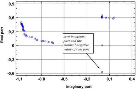
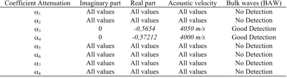
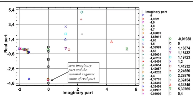
In this example, we will show the variations of the real and the imaginary parts of attenuation coefficients (α3) show in Figure 3 and (α4) show in Figure 4, we will indicate the presence of bulk waves (zero imaginary part and real part is negative) and for a good detection of bulk waves we should have (Imaginary part equals zero and the minimal negative value of real part). We set the value of the real part for (α3), which we will look for it in the Classification as shown Figure 3.

Figure 3. Plot - Real part versus Imaginary part

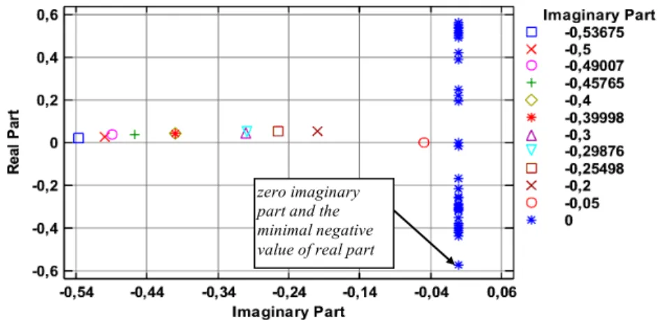
We set the value of the real part for (α4), which we will look for it in the Classification show in Figure 4.

zero imaginary part and the minimal negative value of real part

Re

al

p

art

(6)

Figure 4. Plot - Real part versus Imaginary part 7. RESULTS AND DISCUSSION (for LiNbO3 Lithium Niobate) 7.1. For coefficient attenuation α3

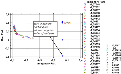
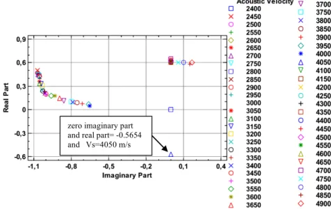
To know the accurate values of each of the real part and the imaginary part which represent coefficient attenuation α3 and Acoustic velocity, Selection variable stays always Acoustic velocity and we change the

Classification factor where we find: show in Figure 5, we have classification where we find classification factor is imaginary part and selection variable is acoustic velocity and number of cases in training set 51, in the minimal negative value of real part we find that the imaginary part equals 0. Show in Figure 6, we have classification where we find classification factor is real part and selection variable is acoustic velocity and number of cases in training set: 51, We find that the minimal negative value of real part equals -0.5654. Show in Figure 7, we have classification where we find classification factor acoustic velocity and selection variable acoustic velocity and number of cases in training set: 51, in the minimal negative value of part part (-0.5654) We find that the acoustic velocity equals 4050 m/s.

Figure 5. Neural Network Bayesian Classifier - Imaginary part (Acoustic velocity)

zero imaginary part and the minimal negative value of real part

Re

a

l p

a

rt

(7)

Figure 6. Neural Network Bayesian Classifier - Real part (Acoustic velocity)

Figure 7. Neural Network Bayesian Classifier - Acoustic velocity (Acoustic velocity)

7.2. For coefficient attenuation α4

Classification factor where we find: show in Figure 8, we have classification where we find classification factor is imaginary part and selection variable is acoustic velocity and number of cases in training set 51, in the minimal negative value of real part we find that the imaginary part equals 0. Show in Figure 9, we have classification where we find classification factor is real part and selection variable is acoustic velocity and number of cases in training set: 51, We find that the minimal negative value of real part equals - 0,57212. Show in Figure 10, we have classification where we find classification factor acoustic velocity and selection variable acoustic velocity and number of cases in training set: 51, in the minimal negative value of part part (- 0,57212) We find that the acoustic velocity equals 4000 m/s.

zero imaginary part and real part= -0.5654

zero imaginary part and real part= -0.5654 and Vs=4050 m/s

(8)

Figure 8. Neural Network Bayesian Classifier - imaginary part (Acoustic velocity)

zero imaginary part and real part= - 0,57212

zero imaginary part and real part= - 0,57212 and Vs=4000 m/s

(9)

Table 1. Summarizes the full work where we can notice bulk waves detection.

Coefficient Attenuation Imaginary part Real part Acoustic velocity Bulk waves (BAW)

α1 All values All values All values No Detection α2 All values All values All values No Detection α3 0 -0,5654 4050 m/s Good Detection α4 0 -0,57212 4000 m/s Good Detection α5 All values All values All values No Detection α6 All values All values All values No Detection α7 All values All values All values No Detection α8 All values All values All values No Detection

8. APPLICATION ON LiTaO3 (Lithium Tantalate)

In this example, we will show the variations of the real and the imaginary parts of attenuation coefficients (α2) show in Figure 11, we will indicate the presence of bulk waves (zero imaginary part and real part is negative) and for a good detection of bulk waves we should have (Imaginary part equals zero and the minimal negative value of real part). We set the value of the real part for (α2), which we will look for it in the Classification show in Figure 11.

Figure 11. Plot - Real part versus Imaginary part 9. RESULTS AND DISCUSSION (for LiTaO3 Lithium Tantalate) 9.1. For Coefficient Attenuation α2

Classification factor where we find: show in Figure 12, we have classification where we find classification factor is imaginary part and selection variable is acoustic velocity and number of cases in training set 51, in the minimal negative value of real part we find that the imaginary part equals 0. Show in Figure 13, we have classification where we find classification factor is real part and selection variable is acoustic velocity and number of cases in training set: 51, We find that the minimal negative value of real part equals -0.5654. Show in Figure 14, we have classification where we find classification factor acoustic velocity and selection variable acoustic velocity and number of cases in training set: 51, in the minimal negative value of part part (-0.5654) We find that the acoustic velocity equals 4050 m/s.

-2 0 2 4 6

Imaginary part -4,6

-2,6 -0,6 1,4 3,4 5,4

Re

al

p

ar

t

Plot of Real part vs Imaginary part

(10)

r ISSN: 2252-8938

IJ-AI Vol. 8, No. 1, March 2019: 33 – 43 42

Figure 12. Neural Network Bayesian Classifier - Imaginary part (Acoustic velocity)

Scatterplot

-2 0 2 4 6

Imaginary part -4,6 -2,6 -0,6 1,4 3,4 5,4 Re al p ar t Imaginary part -2 -1,9321 -1,9 -1,8 -1,7 -1,69001 -1,68011 -1,66 -1,6 -1,59999 -1,58 -1,56001 -1,49231 -1,48454 -1,47654 -1,42987 -1,41232 -1,4 -1,39765 -1,34345 -1,32454 -0,01997 -0,01996 -0,01988 0 1,16874 1,18432 1,19723 1,2 1,41232 2,24656 2,28876 2,32454 4,34345 5,39765 5,4 Scatterplot

-2 0 2 4 6

Imaginary part -4,6 -2,6 -0,6 1,4 3,4 5,4 Re a l p a rt Imaginary part -2 -1,9321 -1,9 -1,8 -1,7 -1,69001 -1,68011 -1,66 -1,6 -1,59999 -1,58 -1,56001 -1,49231 -1,48454 -1,47654 -1,42987 -1,41232 -1,4 -1,39765 -1,34345 -1,32454 -0,01997 -0,01996 -0,01988 0 1,16874 1,18432 1,19723 1,2 1,41232 2,24656 2,28876 2,32454 4,34345 5,39765 5,4 Scatterplot

-2 0 2 4 6

Imaginary part -4,6 -2,6 -0,6 1,4 3,4 5,4 Re a l p a rt -1,9 -1,8 -1,7 -1,69001 -1,68011 -1,66 -1,6 -1,59999 -1,58 -1,56001 -1,49231 -1,48454 -1,47654 -1,42987 -1,41232 -1,4 -1,39765 -1,34345 -1,32454 -0,01997 -0,01996 -0,01988 0 1,16874 1,18432 1,19723 1,2 1,41232 2,24656 2,28876 2,32454 4,34345 5,39765 5,4 Scatterplot

-2 0 2 4 6

Imaginary part -4,6 -2,6 -0,6 1,4 3,4 5,4 Re al p ar t Real part -4,594 -4,19979 -4,18011 -4,14465 -4,12408 -4,08499 -4,08339 -4,07547 -4,00947 -2,34345 -1,41232 -1,4 -1,32454 -0,4 -0,39901 -0,39878 -0,38765 -0,37878 -0,35672 -0,34769 -0,28999 -0,0399 -0,038 -0,035 -0,03454 -0,0328 -0,02987 -0,02888 -0,0276 -0,02448 -0,02001 -0,0128 -0,01001 0 0,02 0,0343 0,0432 0,0723 0,0821 0,09 0,09899 0,3 0,32454 1,0576 1,42987 2,06783 2,09321 3,08 4,0789 5,06987 Scatterplot

-2 0 2 4 6

Imaginary part -4,6 -2,6 -0,6 1,4 3,4 5,4 Re a l p a rt Real part -4,594 -4,19979 -4,18011 -4,14465 -4,12408 -4,08499 -4,08339 -4,07547 -4,00947 -2,34345 -1,41232 -1,4 -1,32454 -0,4 -0,39901 -0,39878 -0,38765 -0,37878 -0,35672 -0,34769 -0,28999 -0,0399 -0,038 -0,035 -0,03454 -0,0328 -0,02987 -0,02888 -0,0276 -0,02448 -0,02001 -0,0128 -0,01001 0 0,02 0,0343 0,0432 0,0723 0,0821 0,09 0,09899 0,3 0,32454 1,0576 1,42987 2,06783 2,09321 3,08 4,0789 5,06987 Scatterplot

-2 0 2 4 6

Imaginary part -4,6 -2,6 -0,6 1,4 3,4 5,4 Re al p ar t Real part -4,594 -4,19979 -4,18011 -4,14465 -4,12408 -4,08499 -4,08339 -4,07547 -4,00947 -2,34345 -1,41232 -1,4 -1,32454 -0,4 -0,39901 -0,39878 -0,38765 -0,37878 -0,35672 -0,34769 -0,28999 -0,0399 -0,038 -0,035 -0,03454 -0,0328 -0,02987 -0,02888 -0,0276 -0,02448 -0,02001 -0,0128 -0,01001 0 0,02 0,0343 0,0432 0,0723 0,0821 0,09 0,09899 0,3 0,32454 1,0576 1,42987 2,06783 2,09321 3,08 4,0789 5,06987 Scatterplot

-2 0 2 4 6

Imaginary part -4,6 -2,6 -0,6 1,4 3,4 5,4 Re a l p a rt Real part -4,594 -4,19979 -4,18011 -4,14465 -4,12408 -4,08499 -4,08339 -4,07547 -4,00947 -2,34345 -1,41232 -1,4 -1,32454 -0,4 -0,39901 -0,39878 -0,38765 -0,37878 -0,35672 -0,34769 -0,28999 -0,0399 -0,038 -0,035 -0,03454 -0,0328 -0,02987 -0,02888 -0,0276 -0,02448 -0,02001 -0,0128 -0,01001 0 0,02 0,0343 0,0432 0,0723 0,0821 0,09 0,09899 0,3 0,32454 1,0576 1,42987 2,06783 2,09321 3,08 4,0789 5,06987 Scatterplot

-2 0 2 4 6

Imaginary part -4,6 -2,6 -0,6 1,4 3,4 5,4 Re al p ar t Acoustic Velocity(Vs) 2400 2450 2500 2550 2600 2650 2700 2750 2800 2850 2900 2950 3000 3050 3100 3150 3200 3250 3300 3350 3400 3450 3500 3550 3600 3650 3700 3750 3800 3850 3900 3950 4000 4050 4100 4150 4200 4250 4300 4350 4400 4450 4500 4550 4600 4650 4700 4750 4800 4850 4900 Scatterplot

-2 0 2 4 6

Imaginary part -4,6 -2,6 -0,6 1,4 3,4 5,4 Re al p ar t Acoustic Velocity(Vs) 2400 2450 2500 2550 2600 2650 2700 2750 2800 2850 2900 2950 3000 3050 3100 3150 3200 3250 3300 3350 3400 3450 3500 3550 3600 3650 3700 3750 3800 3850 3900 3950 4000 4050 4100 4150 4200 4250 4300 4350 4400 4450 4500 4550 4600 4650 4700 4750 4800 Scatterplot

-2 0 2 4 6

Imaginary part -4,6 -2,6 -0,6 1,4 3,4 5,4 Re a l p a rt Acoustic Velocity(Vs) 2400 2450 2500 2550 2600 2650 2700 2750 2800 2850 2900 2950 3000 3050 3100 3150 3200 3250 3300 3350 3400 3450 3500 3550 3600 3650 3700 3750 3800 3850 3900 3950 4000 4050 4100 4150 4200 4250 4300 4350 4400 4450 4500 4550 4600 4650 4700 4750 4800 4850 4900 zero imaginary part and the minimal negative value of real part

zero imaginary part and real part= - 4,594

zero imaginary part and real part= - 4,594 and Vs=3450 m/s

(11)

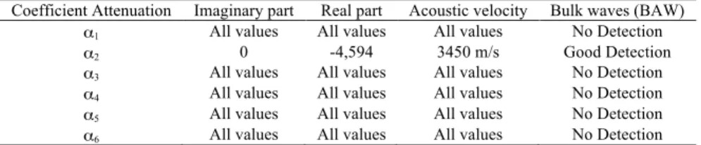
Table 2. Summarizes the full work where we can notice bulk waves detection.

Coefficient Attenuation Imaginary part Real part Acoustic velocity Bulk waves (BAW)

α1 All values All values All values No Detection α2 0 -4,594 3450 m/s Good Detection α3 All values All values All values No Detection α4 All values All values All values No Detection α5 All values All values All values No Detection α6 All values All values All values No Detection

10. CONCLUSION

In this article, we explained that the phenomenon of bulk waves are relying on numerical results at the level of attenuation coefficients. Changes in real and imaginary parts of the coefficients based on the acoustic velocity to detect these waves. Since the bulk waves were detected in Lithium Tantalate (LiTaO3) in one coefficient attenuation α2 and in Lithium Niobate (LiNbO3) were detected in two coefficients attenuation

α3 and α4 so we conclude that (LiNbO3) is the better to use in generating bulk acoustic waves. To compare

between many piezoelectric substrates in detecting acoustic micro waves using PNN classification you just have to change the characteristics of the material parameters, and those results we need them in realization of acoustic microwaves devices.

REFERENCES

[1] Spaldin NA, Cheong S W and Ramesh R,Multiferroics : Past, present, and future, Phys. Today, Vol 63,2010, pp 38-43.

[2] Tao Yan, Ning Ye, Liuwei Xu, Yuanhua Sang, Yanxue Chen, Wei Song, Xifa Long, Jiyang Wang and Hong Liu, Ferromagnetism in chemically reduced LiNbO3 and LiTaO3 crystals, Journal of Physics D : Applied Physics, 2012, Vol 49, 195005.

[3] T. Hatanaka, K. Nakamura, T. Taniuchi, H. Ito, Y. Furukawa, K. Kitamura, Quasi-phase-matched optical parametric oscillation with periodically poled stoichiometric LiTaO 3, Optics Letters, Vol 25,2000, pp 651-653.

[4] J.C. Wu, Z.B. Chen, R.K. Choubey, C.W. Lan, On the study of zinc doping in congruent LiTaO3 crystals, Materials Chemistry and Physics, Vol 133, 2012, pp 813-817.

[5] Daniel Royer and Eugene Dieulesaint, Elastic Waves in Solids II – Generation, Acoustic-optic Interaction, Applications, Springer-Verlag, New York (1999).

[6] Mingxi Deng, Simulation of Generation of Bulk Acoustic Waves by Interdigital Transducers, IEEE Ultrasonics Symposium, Vol 1, 2001, pp 855-858.

[7] Ken-ya Hashimoto, Masatsune Yamaguchi, Gunter Kovacs, Karl Christian Wagner, Werner Ruile, and Robert Weigel, Effects of the Bulk Wave Radiation on IDT Admittance on 42o_YX-LiTaO3,_{IEEE Transactions on} Ultrasonics, Ferroelectrics, and Frequency Control, Vol 18, No 5, pp1419-1425, 2001.

[8] D. Benatia and M. Benslama, “Analysis of Leaky and Bulk Acoustic Microwaves by Wavelet Technique,” Journal of Communications in Numerical Methods in Engineering, U.K, Vol 16, pp165-175, 2000.

[9] H. Hafdaoui and D. Benatia, Identification of Acoustics Microwaves (Bulk Acoustic Waves) in Piezoelectric Substrate (LiNbO3 Cut Y-Z) by Classification Using Neural Network, Journal of Nanoelectronics and Optoelectronics, Vol 10, No 03, pp 314-319, 2015.

[10] D. Benatia and M. Benslama, Identification of bulk microwaves and detection of Pseudo singularities by wavelet technique in piezoelectric medium, International Journal of Electronics, Vol 93, No 8, August 2006, pp 567–579. [11] D.Benatia, Modélisation des ondes de volume rampantes sous la surface (SSBW) par une technique mixte ondelettes

et fractales, Thèse de Doctorat d’Etat, Université de Constantine, institut d’électronique, 1999.

[12] I. D. Avramov: "High Q metal strip SSBW resonator using a SAW design", IEEE Transactions on ferroelectrics and frequency control, Vol 37, pp 530-534, 1990.

[13] D. Benatia et M. Benslama - Identification des Ondes de fuite et de volume dans les Matériaux piézoélectriques. Cas du Niobate de Lithium (LiNbO3 Coupe Y-Z) ‘’ 3rd International conference: Sciences of electronic, technologies of Information and telecommunications March 27-31, 2005 – TUNISIA’’

[14] D. Benatia, T. Fortaki et M. Benslama -Détection des ondes de fuite dans les matériaux piézoélectriques ‘’ 4th International conference: Sciences of electronic, technologies of information and telecommunications March 25-29, 2007 – TUNISIA’’

[15] H.Hafdaoui, Détection et génération des micro-ondes acoustiques de volume dans les structures piézoélectriques, Thèse de Doctorat, Université de Batna 2, 2016.

[16] Pv Nageswara Rao, T Uma Devi, Dsvgk Kaladhar, Gr Sridhar, Allam Appa Rao, “A Probabilistic Neural Network Approach for Protein Superfamily Classification ‘‘Journal of Theoretical and Applied Information Technology, Vol 6, No1, pp 101-105, 2009.

[17] L.Abdelhadi, R.Tlemsani, A. Benyettou. “Un Nouvel Algorithme d‘Apprentissage pour les Réseaux Probabilistes”, 11th African Conference on Research in Computer Science and Applied Mathematics. pp 208-215. 2012.