Oviedo University Press 208 ISSN: 2254-4380
Economics and Business Letters 3(4), 208-217, 2014
An eigenvector spatial filtering contribution to short range regional
population forecasting
Daniel A. Griffith* • Yongwan Chun
University of Texas at Dallas, USA
Received: 8 October 2014 Revised: 15 December 2014 Accepted: 28 December 2014
Abstract
Statistical space-time forecasting requires sufficiently large time series data to ensure high quality predictions. The dominance of temporal dependence in empirical space-time data emphasizes the importance of a lengthy time sequence. However, regional space-time data often have a relative small temporal sample size, increasing chances that regional forecasts might result in unreliable predictions. This paper proposes a method to improve regional forecasts by incorporating spatial autocorrelation in a generalized linear mixed model framework coupled with eigenvector spatial filtering. This methodology is illustrated with an application to regional population forecasts for South Korea.
Keywords: eigenvector spatial filter, population, South Korea, space-time forecasting, spatial
autocorrelation
JEL Classification Codes: C21, P23, R23
1. Introduction
Consider a geographic landscape comprising n areal units (e.g., counties) and T points in time. This is a panel data structure (Baltagi, 2013). Space-time forecasting of population counts is an important problem that can be solved statistically with a sufficiently large dataset, or with population projection matrices coupled with a sequence of T-1 n-by-n inter-areal unit migration flows data. Because space-time statistical forecasts tend to be dominated by time dependence
* Corresponding author. E-mail: [email protected].
3(4), 208-217, 2014 209 (Griffith, 2013), T needs to be relatively large. Meanwhile, as n increases, geographic heterogeneity compromises the simplicity of a space-time statistical forecast. In contrast, collecting areal unit migration data is an onerous and costly task that dissuades the construction of population projection matrix forecasts.
When T is relatively small (e.g., << 50), and points in time are relatively close together (e.g., 1 year apart), estimated time series statistical forecasting models tend to be unreliable, and resources rarely are spent to repeatedly collect migration data over such a short time horizon. In this context, recognizing that spatial autocorrelation is a manifestation of the inertia—i.e., the resistance to change—in a space-time geographic landscape arising from temporal dependence, spatially structured and spatially unstructured random effects can be estimated separately and then used to make forecasts. The purpose of this paper is to describe this advance in regional forecasting. This furnishes a supplemental approach to panel data analysis for large n, small T, and unobserved heterogeneity.
2. Methods
The set of methods employed for data analysis purposes here includes principal components analysis (PCA), Box-Jenkins time series modelling techniques, eigenvector spatial filtering, and generalized linear mixed model techniques. To adjust for variation in the size of areal units, population counts are converted to densities.
A sequence of annual population density maps for a given geographic landscape tends to display extremely large positive Pearson product moment correlation coefficients. PCA furnishes one multivariate statistical method for confirming this feature of a space-time dataset, and quantifying its magnitude. In this context of highly correlated maps, when the time series is relatively short (e.g., T = 12), an estimated first-order autoregressive parameter, denoted by AR(1), tends to be near the upper limit of its feasible parameter space (i.e., close to 1). Meanwhile, as n increases, the variability of the n AR(1) values tends to increase, and more and more areal units tend not to be characterized by the average of these AR(1) values.
Eigenvector spatial filtering (see Chun and Griffith, 2013) employs selected eigenvectors extracted from an n-by-n spatial weights matrix C, which articulates the correlation structure for geographic locations across space, as synthetic proxy variables that can be used to control for residual spatial autocorrelation by filtering it out of the model residuals and transferring it to the mean response term. These control variables identify and isolate the stochastic spatial dependencies among a set of georeferenced observations, resulting in independence being mimicked, and thus allowing model estimation to proceed as though the observations are independent. The most popular implementation of eigenvector spatial filtering uses an eigenfunction decomposition of the matrix version of the Moran Coefficient (MC) numerator
(I – 11′/n)C(I - 11′/n) (1)
where 1 is an n-by-1 vector of ones, and ′ denotes the matrix transpose operator. This decomposition generates n eigenvectors, say E = (E1, E2, E3, …, En), and their associated n eigenvalues, say λ = (λ1, λ2, λ3, …, λn), where the subscript represents a descending ordering by eigenvalue value. These eigenvalues enable calculation of the MC for their corresponding n-by-1 eigenvectors: MCj = T λj
n ⋅
C1
Daniel A. Griffith and Yongwan Chun Short range regional forecasting
3(4), 208-217, 2014 210 A generalized linear mixed model (GLMM) is a statistical model built upon both normal and non-normal probability models, with a mean response whose relationship with a linear combination of covariates and a random effects term is defined by a link function, say g (McCulloch, Searle, and Neuhaus, 2008). For simplicity, these random effects frequently are assumed to conform to a zero mean normal distribution. They often are specified with both spatially structured and unstructured components for georeferenced data. Let Yi be a response variable, Xi be a 1-by-(p+1) vector of p covariates and a 1 (for the intercept term), and Zi be a design matrix (e.g., defining repeated measures through time) for observation i. Then
)
ξ
( g ) (
g
µ
)
E(Yi = i = −1 XiβX +Ziγ = −1 XiβX +Ek,iβE + i+Wi , (2)
where E denotes the calculus of expectation operator, βX is a (p+1)-by-1 vector of covariate
regression coefficients (including the intercept term), βE is a k-by-1 vector of selected eigenvector regression coefficients, with Ek,iβX being a spatially structured random effects term,
ξ is a spatially unstructured random effects term, and Wi is the sum of q>0 offset variables (which, by definition, have coefficients of 1).
3. Data
The foundational space-time dataset is for 12 years of resident population counts (1997-2008) across South Korea’s 230 Si-Gun-Gu (which are similar to counties). These population counts are available from a South Korean government database containing the residential locations of people in South Korea. This resident registration is compulsory in the country, and address changes by residents must be reported to the government.1 Jeju Iisland is partitioned into two Si-Gun-Gu that are not linked to the mainland in the geographic weights matrix. Figure 1a portrays aggregate annual population growth for South Korea as a whole across the 1992-2013 time horizon, together with the Korean quinquennial census population counts since 1925. The two overlapping trajectories are nearly parallel, and roughly linearly related to time (Figure 1a). Because the resident population includes people who temporarily live in other counties due to, for example, their jobs or being students, resident population is slightly larger than its corresponding census population counts.
1 Three different national population statistics are available in South Korea: (1) resident population from the Ministry
of Security and Public Administration, (2) census population from Statistics Korea, the Korean national statistical office, and (3) population projections from Statistics Korea. These data can be accessed at
3(4), 208-217, 2014 Figure 1. Statistical characteristics of the space
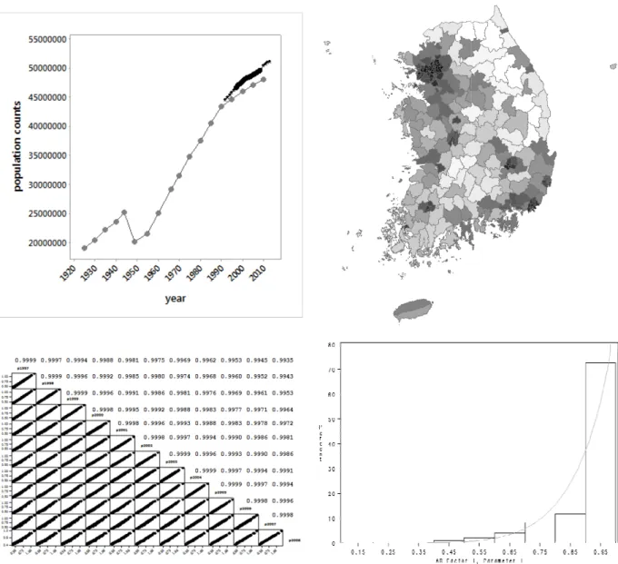
Top left (a): the aggregate South Korea population time series: gray denotes quinquennial census counts, black asterisks denotes resident population
space-time forecasting model.
Top right (b): the geographic distribution of the first principal component scores (MC = 0.76297); score value directly related to grayscale darkness.
Bottom left (c): scatter plot and correlation matrix for the 12 maps.
Bottom right (d): the frequency distribution of the AR(1) coefficients, with a superimposed beta distribution curve.
Figure 1. Statistical characteristics of the space-time series
Top left (a): the aggregate South Korea population time series: gray denotes quinquennial census counts, black resident population counts, and solid black circles denote the foundation years used to estimate the
Top right (b): the geographic distribution of the first principal component scores (MC = 0.76297); score value le darkness.
Bottom left (c): scatter plot and correlation matrix for the 12 maps.
Bottom right (d): the frequency distribution of the AR(1) coefficients, with a superimposed beta distribution curve.
211 Top left (a): the aggregate South Korea population time series: gray denotes quinquennial census counts, black counts, and solid black circles denote the foundation years used to estimate the
Top right (b): the geographic distribution of the first principal component scores (MC = 0.76297); score values are
Daniel A. Griffith and Yongwan Chun Short range regional forecasting
3(4), 208-217, 2014 212
4. Results
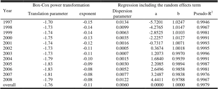
The population densities (population/area) were subjected to a Box-Cox power transformation— namely, 1/(density-1.76)0.11—so that they better conform to a bell-shaped curve, a procedure that moderates impacts of outliers2. The individual year translation and exponent parameters display a time trend (Table 1). A PCA of the 12 transformed population density maps produces a single component accounting for 99.85% of the variance in these maps. In other words, the 12 maps are highly multicollinear, and are nearly identical in their map patterns (Figure 1c). Figure 1b portrays the composite map pattern for these transformed population densities.
Table 1. Selected estimation results for the individual population maps
Year
Box-Cox power transformation Regression including the random effects term
Translation parameter exponent Dispersion
parameter a b Pseudo-R
2
1997 -1.70 -0.15 0.0134 -5.7201 1.0247 0.9946
1998 -1.73 -0.14 0.0099 -4.2765 1.0147 0.9967
1999 -1.74 -0.14 0.0063 -2.8525 1.0103 0.9981
2000 -1.75 -0.13 0.0035 -2.2257 1.0127 0.9991
2001 -1.74 -0.12 0.0016 -0.7317 1.0071 0.9993
2002 -1.73 -0.11 0.0005 0.3674 1.0018 0.9995
2003 -1.73 -0.11 0.0007 1.2073 0.9970 0.9996
2004 -1.79 -0.10 0.0015 1.6840 0.9939 0.9991
2005 -1.83 -0.09 0.0030 2.2085 0.9894 0.9987
2006 -1.83 -0.08 0.0052 2.6496 0.9858 0.9981
2007 -1.81 -0.08 0.0077 3.2487 0.9838 0.9976
2008 -1.79 -0.08 0.0122 4.4411 0.9788 0.9967
overall -1.76 -0.11 0.0060 0.0000 1.0000 0.9979
Next, AR(1) models were estimated for each of the n = 230 (T = 12) time series of these transformed values (Figure 1d). Over 50% of the serial correlation parameter estimates exceed 0.95 in value. But some of the values are as small as roughly 0.16. Moreover, the distribution of the values conforms well to a Beta random variable with parameters 8.1 and 0.9. These properties coupled with only 12 points in time are antithetical to establishing sound time series forecasting.
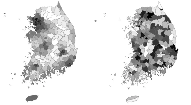
Consequently, Eq. 2 was estimated, with the response variable population being a count, and the covariates being a log-area offset variable (i.e., its coefficient was set to 1)—this specification is equivalent to an untransformed population density described by a non-normal probability model—and the intercept term. The link function g was defined in terms of a negative binomial (i.e., Poisson with a gamma distributed mean) probability model. This specification accounts for nearly all of the variability in population density across South Korea (Table 1). The random effects term has a mean of -0.0060, but deviates from normality according to its Shapiro-Wilk diagnostic statistic. Its spatially structured component (Figure 2a) is an eigenvector spatial filter (ESF) constructed with 25 vectors that account for 80% of its variability. Its spatially unstructured component (Figure 2b) still has a mean of -0.0060, but conforms closely to a normal
2
3(4), 208-217, 2014 213 distribution (its Shapiro-Wilk statistic probability is 0.2465); this term represents heterogeneity across the South Korean geographic landscape. These individual spatially structured and unstructured random effects terms are the same for every point in time, which accounts for the strong pairwise correlations among the twelve maps (Figure 1c). Respecifying the random effects term with a space-time filter (Griffith, 2012) fails to change these results, an outcome that is consistent with the preceding PCA and AR(1) findings.
Figure 2. The random effects terms
Left (a): the spatially structured random effects (MC = 0.98259) Right (b): the spatially unstructured fandom effects (MC = 0.04931)
Areal unit values are directly proportional to grayscale darkness.
Daniel A. Griffith and Yongwan Chun Short range regional forecasting
3(4), 208-217, 2014 214 heterogeneity terms become more important, with the passing of time. Therefore, forecasts can be constructed for time t+k by rescaling the estimated model results as follows:
k t i,
Pˆ + = Areai exp(4.1725 + ESFi + ξˆi)
∑
∑
=
= +
+ + 230
1 i
i i i
230
1 i
k t i,
)
ξˆ
ESF exp(4.1725 Area
P
, (3)
where Pi,t is the population of areal unit i are time t, Areai is the area of areal unit i, and ESFi is the ESF value for areal unit i. Eq. 3 requires a total population figure, Pt+k =
∑
= + 230
1 i
k t i,
P , which can be a short range aggregate forecast. Mean squared error (MSE) calculations based upon Eq. 3 again emphasize that the estimated spatially structured and spatially unstructured random effects terms best describe the midpoint of the space-time series (Figure 4a), and hence the equation’s restriction to producing only short range forecasts, which becomes a necessary tool when time series are very short. This conclusion does not change by using the year-specific bivariate GLMM coefficients because the random effects terms are estimated with the entire foundational time series. For example, the 2008 year-specific results yield an increase in the MSE of 12.4%. The best case scenario is for 2006, for which the MSE decreases, but by only 1.1%. Spatially structured random effects can be estimated without a time series, although a single-year estimate may contain some biased; but the spatially unstructured random effects term, which here accounts for roughly 20% of the variability in the total random effects term, cannot.
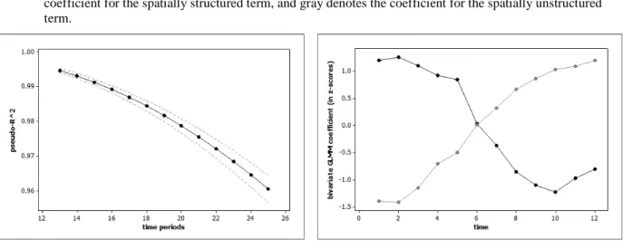
Figure 3. Time series for model goodness-of-fit statistics and parameter estimates for population densities
Left (a): forecasted R2 values with prediction intervals.
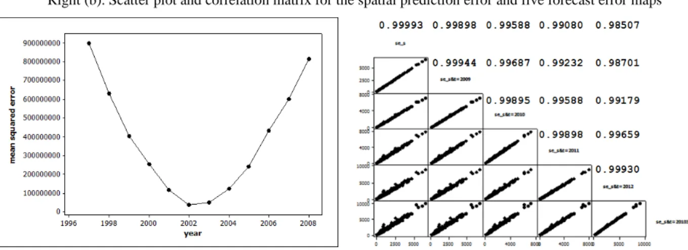
3(4), 208-217, 2014 215 Figure 4. Time series for model goodness-of-fit and population density forecast prediction error
Left (a). The MSE for the population maps based upon the forecast Eq. 3
Right (b). Scatter plot and correlation matrix for the spatial prediction error and five forecast error maps
The annual space-time results for 2009-2013 can be analyzed to assess the quality of population count estimates presented by Eq. 3 estimated with data for 1997-2008. A simple Box-Jenkins time series forecast based upon the annual total population counts for South Korea during 1992-2008 (Figure 1a) yields
2 t 1
t
t (1 0.85401) 344381.2 (1 0.85401)P 0.85401P
Pˆ = − × + − − + − , (4)
where Pt denotes the population of South Korea at time t, a first differencing was done, the first-order autoregressive parameter estimate is 0.85401, and the mean of the differenced series (with only 17 points in time) is 344381.2. Residual diagnostics suggest that only trace serial correlation remains. Table 2 reports the forecasts for the subsequent five years, which are reasonably good given the shortness of the time series. The pseudo-R2 values are better than expected (Figure 3a), and are identical for the observed and forecasts because the forecasts are simply a rescaling of the predicted values corresponding to the observed counts. On average, the MSEs for the forecasts are more than 20% greater than their corresponding MSEs for the predicted values. This reflects the sizeable prediction error for the forecasted 1997-2008 total population: the variance of the space-time distribution of values has an error term for the forecasts multiplied by an error term for the predicted values; this latter error component is constant over time, whereas this former error component increases across a forecast horizon. Figure 5a presents the 2009 space-time population counts forecast; Figure 5b portrays the geographic distribution of its spatial prediction error. This result can be extended to space-time forecasts by the mathematical statistics theorem (Goodman, 1962) about the variance of the product of two independent random variables (i.e., the time series forecasts here are independent of the spatial forecasts), which equals
∑
= + + + + 230 1 i i i i 2 s 2 T 2 T 2 s 2 T 2 s ) ξˆ ESF exp(4.1725 Area σ µ σ µ σσ i i i
, (5)
where the denominator
∑
= + + 230 1 i i i iexp(4.1725 ESF ξˆ )Area = 48,212,412 and can be assumed fixed
here because it does not change from forecast to forecast, 2 T
Daniel A. Griffith and Yongwan Chun Short range regional forecasting
3(4), 208-217, 2014 216 series forecast (from Table 2), µT denotes the forecasted time series value (i.e., its mean; from Table 2), σ2si denotes the spatial variance for areal unit i (portrayed in Figure 5b), and µsi denotes the spatial mean for areal unit i (portrayed in Figure 5a). The time series forecasting uncertainty approximately multiplies each of the areal unit prediction standard errors by the following factors:
year 2009 2010 2011 2012 2013
factor 1.05013 1.11160 1.21758 1.36293 1.53854
In other words, the map in Figure 5b essentially retains its geographic pattern, but with rescaled values (Figure 4b).
Table 2. Selected summary statistics for the forecasts
Year Total population forecast Observed total Forecast total
Forecast Standard error In 95% CI R2 MSE R2 MSE
2009 49822455 60988 Yes 0.9956 815827242 0.9956 1032494759
2010 50113636 128471 No 0.9950 1034744617 0.9950 1310487901
2011 50412584 203292 Yes 0.9938 1287201916 0.9938 1566867185
2012 50718165 282071 Yes 0.9932 1550314549 0.9932 1844516609
2013 51029410 362684 Yes 0.9923 1833486681 0.9923 2150340770
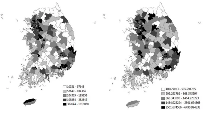
Figure 5. The geographic distribution of 2009 space-time-based population count forecasts and their uncertainty
3(4), 208-217, 2014 217
5. Concluding remarks
This paper summarizes an advance in short run space-time regional population forecasting when existing time series contain relatively few observations and points in time are close together. This advance exploits spatial autocorrelation as well as random effects in a GLMM framework to geographically distribute aggregate population over areal units of a geographic landscape. The spatial autocorrelation component is approximated with an ESF, which captures the complex map pattern portraying spatial dependence that is latent in population counts, and preserves it in regional forecasts of population. As such, this paper differs from Griffith and Paelinck (2009) in four ways: (1) it treats a substantially larger number of areal units (230 rather than 11); (2) it evaluates forecasts with observed data (rather than output from a spatial econometric model); (3) it derives prediction error maps to accompany population forecast maps; and, (4) it analyzes South Korean population counts (rather than Belgian economic value added figures).
One surprising outcome from the analysis summarized here is that the quality of the regional forecasts is better than expected, given diagnostics such as Figure 3. A second is that the two time components in expression (5) do not dominate the prediction error maps. A third is that although time dependence almost always dominates spatial dependence in practice, results summarized here demonstrate that such temporal dominance can materialize through inertia in spatial dependence as captured by a spatially structured random effects term.
Empirical evaluations of the short run population forecasts indicate that using an ESF to describe spatially structured random effects coupled with a spatially unstructured random effects term furnishes good annual county-level geographic resolution predictions for several years into the future. Similar evaluations need to be conducted for other countries and other geographic resolutions.
Acknowledgements. We thank Monghyeon Lee and Hyeongmo Koo for their assistance in collecting the South Korea population dataset.
References
Batalgi, B. (2013) Econometric Analysis of Panel Data, 5th ed., Wiley: New York.
Chun, Y. and Griffith, D. (2013) Spatial Statistics & Geostatistics, SAGE: Thousand Oaks, CA. Goodman, L. (1962) The variance of the product of K random variables, Journal of the American
Statistical Association, 57, 54-60.
Griffith, D. (2012) Space, time, and space-time eigenvector filter specifications that account for autocorrelation, Estadística Española, 54(177), 7-34.
Griffith, D. (2013) Estimating missing data values for georeferenced Poisson counts,
Geographical Analysis, 45, 259-284.
Griffith, D. and Paelinck, J. (2009) Specifying a joint space- and time-lag using a bivariate Poisson distribution, Journal of Geographical Systems, 11, 23-36.