Technology Implications of UWB on Wireless
Sensor Network-A detailed Survey
Kamran Ayub
1, 2, Valerijs Zagurskis
21
Technology Group, NYUAD Saadiyat Campus New York University.
2
Institute of Electronics and Computer Science, Riga Technical University, Latvia. [email protected], [email protected]
Abstract – In today’s high-tech “SMART” world, sensor-based networks are widely used. The main challenge with wireless-based sensor networks is the underneath PHY (physical) layer. In this survey, we have identified core obstacles of wireless sensor network when UWB (Ultra-Wideband) is used at PHY layer. A systematic approach is used to assess the effectiveness of UWB for WSN (Wireless Sensor Network). Multiple information sources (surveys, research papers, articles, books and technical surveys) were consulted. Our aim is to measure the UWB’s effectiveness for WSN and analyze the different obstacles allied with its implementation. Here focusing on the core concerns (e.g., spectrum, interference, and synchronization) we started our research by reviewing existing solutions and end up with our findings of the new theories.
Our research concludes that despite all the bottlenecks and challenges, UWB’s efficient capabilities makes it an attractive PHY layer scheme for the WSN, provided we can control interference and energy problems. This survey gives a fresh start to the researchers and prototype designers to understand the technological concerns associated with UWB’s implementation.
Keywords – Impulse Radio, Media Access Control, Ultra-Wideband, Wireless Sensors Network.
1.
Introduction
Throughout the last decade, our view and utilization of information transportation both have drastically changed. Since the new era of communication technology started, UWB has been one of the leadings research topics in the communication community [1], [2]. Researchers are examining its effectiveness in various directions. Though UWB can be used in a broad range of applications, the prominent one is the sensor network (e.g., WSN) [3]–[5]. WSN’s physical layer has many unique requirements. It requires a simple energy efficient, robust link, a light transceiver architecture, and simple but reliable synchronization. Last but not the least is overall energy consumption by the network. Researchers has multiple opinions on UWB’s effectiveness. Some of them do not think that there is any value behind this light power communication alternative, but most of them are positive about its effectiveness. Outcomes of the literature show that UWB is a perfect platform for WSN-applications [6]–[10]. One of the interesting quality of UWB communication system is its low power consumption that makes it attractive for both types of UWB, OFDM (Orthogonal frequency division multiplexing) and IR (Impulse Radio). UWB’s implementation is simple and economical. Its resistance to interference with other systems and time domain resolution make it a perfect platform for wireless sensor network. In
industry, common examples are location-based networks, imaging based applications [5], intrusion prevention systems [6], surveillance [7], traffic radar systems [8], sports monitoring [11], hydrographic systems, and other civil infrastructure [12]. Due to UWB’s harmless effect on human body, UWB is also found as an alternative to the other Medias which may affect human body in WBAN (Wireless Body Area Network). Due to these added values, UWB is an active research topic in both the industry and the government/military domain. Many famous labs, BT-Labs Ipswich London, US Army Research Labs, and DOCOMO Research lab USA has active research projects on UWB. The research about the physical layer (802.15.4a standard) has very promising results [13] and a precise PHY and MAC layer solution for (most of the) WSN applications.
From the recent research, it was observed that most of the advanced issues with the Wireless Sensor Network are related to Physical layer or Radio Layer. Compatibility with physical layer and low duty cycle are the essentials for a WSN. Spread Spectrum and Narrow Band both have been successfully implemented with the conventional networks, Wi-Fi (802.11) and ZigBee (802.15.4) both standards are based on Spread Spectrum but unfortunately with sensor network they have serious technical issues. For example, ZigBee is a low power solution but it has support limitation and does not support more than 50 nodes. Similarly, though Wireless HART is a globally recognized platform but its compatibility with WSN’s protocols is an issue. Also Wi-Fi and Bluetooth both have very high power consumption. These issues are not limited to, power consumption at transceiver but also at resource management (due to the large number of nodes). Narrowband on the other hand has various limitations. One of the major issues with Narrowband is MUI (Multi user interference) and data rate is also serious concern.
Inability of Narrow Band and Spread Spectrum to fulfill modern wireless sensor network requirements, research turned towards Ultra Wideband (UWB). Due to the low transmission power, UWB signal does not interfere with Narrow band radio communication, also it saves energy that is the basic need of a wireless sensor node. Ultra-wideband was also found as an alternative for the short range data communication both indoor and outdoor environments.
Core technology implications are explained in Section 4. Section 5 wraps up this paper by highlighting open research concerns.
2.
Technical Background
2.1 Overview of WSN
In wireless sensor networks, transceivers (paired with sensing circuitry) are used to transmit sensed data (e.g., temperature and humidity) to the sink. Nodes comprises of transceivers (and other related circuitries) need to be inexpensive and less complex so that they can easily be deployed in any desired area. The goal is to transmit sensed data to the hub reliably without any issue. For that reason communication among nodes is usually in an ad-hoc fashion, and the communication infrastructure is not fixed. Data transmission from a source node to the destination in a WSN may go via multiple hops, where some nodes have limited jobs, e.g., relaying. To design a wireless sensor network following are the fundamental requirements. See the HLD (high-level design) of WSN Figure 1.
Economical: A single node’s cost defines the overall cost of
a solution. Thus, it is important to keep the node’s cost affordable. Nodes are usually in the count of hundreds to thousands thats why price matters. Another important point is the lifetime of a node; usually nodes retire as the battery ends its life.
Power depletion: Nodes in WSN usually have to run for
years and years, and as the battery gets drained they are considered retired. Hence, it is crucial that the network should be designed in a way that it can keep its battery life according to the original project plan.
SFP (Small Form-factor Pluggable): Transceivers in WSN
need to be built on small form factor so they can offer high speed and compactness. SFP transceivers have to be hot swappable [14] so that they can be deployed to any location easily.
Robustness: Managing abnormality during transmission is
an important feature of any network, and it is a core requirement of a Wireless Sensor Network. In an ideal network, the node must have the ability to tackle the environmental challenges, e.g., fading and shadowing. Robustness is directly proportional to the network lifetime.
Figure 1. High Level Design of WSN-Communication Data rate: Data rate is an important component of WSN
design. Though wireless sensor network works on low data rate, some complex multimedia (streaming type) sensor networks may require medium to high data-rate. Based on
data rate requirements, design of WSN topology has to be planned.
Hybrid Structure: Intelligent circuitry has made our
networks more intelligent than ever, today wireless sensor network is used in a versatile fashion with multiple capabilities. Where some nodes are sensing temperature, others are measuring pressure. The Hybrid WSN (Heterogeneous Wireless Sensor Network) is already in the market. So, network design should support hybrid feature at the design level.
These are the primary requirements of a wireless sensor network design; some other secondary requirements could be energy compatibility, design flexibility, and platform efficiency.
2.2 WSN Design Issues and Requirements
High-level design of a wireless sensor network Figure 1 shows a distinctive architecture of a WSN Node. Network is comprise of small tiny nodes, and their role is divided into several categories. Some are working on real sensors. Some are just as relay masters (to forward data to the next hop). A few work as SINK (for data processing and scheduling) and are linked with other networks (e.g., the internet) via a gateway. Wireless is used as a medium among nodes for the connectivity. To understand the design requirements of a WSN, one has to compare it with the conventional data network. WSN differs from traditional data networks. The followings are the common differences.
• The number of nodes (used) in WSN is between hundreds to thousands.
• In Wireless Sensor Networks, nodes’ deployment is under tough environmental conditions.
• The battery life of WSN nodes is final and at the end of battery life, batteries are not replaced.
• The topology of nodes in WSN differs significantly from the traditional network as the aim is to make sure that the death of one node does not compromise the performance of the rest of the network.
Following are the core design constraints in details. 2.2.1 Resiliency (Consistency):
WSN has to be conceived in a way that the death of one node should not impact the availability of the whole network. Resiliency keeps regular network operations alive even in case a node is down. During the design phase of WSN, it is important to make sure that there is an acceptable level of redundancy available. Following equation is used for the resiliency calculation, this is analytically modeled by the author in [15].
( )
(
)
k k
R t = exp −λ t (1)
Here R = resiliency (redundancy), k λk= fault rate of node k and t = time period.
2.2.2 Scalable Design:
change (increase/decrease) this. The following formula is used for scalability calculation.
δ
( )
r = NA / R (2) Here (area)A=π r2 & “R” is the coverage area. N shows (number of) nodes/sensors. δ(r) counts the required number of nodes in a specified coverage area (range).2.2.3 Hardware Constraints:
Looking at a node structure (Figure 2), we can see various parts (embedded within the chipset). Such as,
• Sensing Unit (e.g., Analog to digital converter and sensor)
• Microcontroller/ Processing Unit
• Memory
• Radio Transceiver unit.
Figure 2. Generic block diagram of a WSN-Node [16]
All these major parts contribute to the overall performance of WSN. In the next section we will review the major hardware constraints for WSN.
(a) Energy
Energy or power management in wireless sensor network depends on two important parts, technology (behind the battery) and its operational utilization. From the available technologies, we have three options, Alkaline, Lithium, and Nickel. All three types have their limitations and drawbacks. For example, Alkaline is a cheap solution but size and wide voltage range are the weaknesses. Similarly, Lithium is a compact solution but the low nominal discharge current is an issue. Nickel Hydride is the third option. Though they are rechargeable but due to decreasing in energy density, they do not fit for Wireless Sensor Networks.
(b) Transceiver
LPT (Low power Transceiver) is a common choice for WSN. However, research shows that the low power transceivers consume almost the same amount of power (as conventional radios) when they are in “Tx” or “Rx” mode. Therefore use of
effective scheduling algorithm at MAC (Medium Access Control) is crucial. Inside the transceiver, both transmitter and receiver consume almost the same amount of power. Aside from major parts, Mixer, Voltage Oscillator, and Amplifier also consume limited energy. They need power in addition to the START up power; START up plays a significant role in energy saving. Therefore, it is considered an important parameter for the MAC design (where Transceiver’s scheduling is defined). Startup power can be calculated by the following formula [17].
(
)
( )
(
)
(
)
C T T on ST out on R R on st
P =N P T +T +P T +N [ P R +R (3)
Here, PT, PR represent transmitter and receiver power
respectfully, Pout is power at transmitted antenna.
on on
T and R are the transmitter and receivers’ wake up time,
similarly T and R are Transmitter and receivers’ startup st st time. N / N Are the switching b/w “On” and “Off” states T R of the transceiver and depends on (MAC) scheduling. In case of Radio’s power distribution, antenna consumes very less power compared to the operational part. Transmission range is a major factor here. Longer transmission range means more energy for the radio. For the selection of radio, which is “fit for purpose”, encoding algorithm and antenna gain are the two additional areas of consideration [18].
Figure 3. UWB pulses (modulated and at Correlator)
(c) Processing Unit
Data processing is performed prior to the data communication. In recent advancement due to chip integration in a the microprocessor, the power consumed during this phase is lesser than the data communication phase. That makes them a perfect choice for the Wireless Sensor Network. Besides the cost and the functionality of these modern circuits, they are versatile and compatible with WSN. As Power is the main constraints of Wireless Sensor Network, research shows that the most substantial processing structure is CMOS (complementary metal-oxide semiconductor), that gives better efficiency by limiting the depleted power.
Along all the above aspects, financial constraints are also very crucial. It is important to keep the overall network budget in control at all times.
3.
UWB Compatibility with WSN
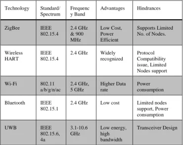
Ultra Wideband due to its properties is a solid candidate for the Wireless Sensor Network. Though narrow band transmission schemes under WSN, e.g., DSSS (direct sequence spread spectrum) are widely used and is very effective under 2.4 GHz band their performance matrix is lesser than the Ultra Wideband. Major disadvantages of these transmission technologies are statistically explained in the following table, Table 1.
Table 1. UWB vs. Existing Technology Solutions
Technology Standard/ Spectrum
Frequenc y Band
Advantages Hindrances
ZigBee IEEE
802.15.4
2.4 GHz & 900 MHz
Low Cost, Power Efficient
Supports Limited No. of Nodes.
Wireless HART
IEEE 802.15.4
2.4 GHz Widely recognized
Protocol Compatibility issue, Limited Nodes support
Wi-Fi 802.11
a/b/g/n/ac
2.4 GHz, 5 GHz
Higher Data rate
Power consumption Bluetooth IEEE
802.15.1
2.4 GHz Low cost Limited nodes support, Power consumption
UWB IEEE
802.15.6, 4a
3.1-10.6 GHz
Low energy, high bandwidth
Transceiver Design
By comparing the UWB’s properties with the sinusoidal carrier-based system, the following are the UWB’s advantages.
• Data Transmission Rate: Very High
• Space Frequency Spectrum: Superb efficiency.
• Probability of Interception: Very Low
• Distance Measurement: High precision
• Power Consumption: Very Low
• Cost: Very Low
• Implementation: Easy/Moderate
Figure 4. Different wireless standards in ISM Bands [19]
In the next section Ultra Wideband strength are explained in more details.
3.1 Strengths of UWB for Wireless Sensor World
Narrow band is a common solution for conventional networks, but it does not fulfill all the requirements of the sensor network, especially WSN’s connectivity requirements. On the other hand, UWB is lightweight platform, hence detection and interception of UWB signal (due to the low “Tx” power) is relatively complex Figure 3.
Ultra Wideband is less complex and more reliable that makes it very suitable for WSN.
3.1.1 Energy Efficient, economical and simple
Transceiver Circuitry
UWB is not a new technology, but its use in Wireless Sensor Networks is just a few years old. It uses narrow pulses and a wide frequency spectrum for the transmission.
So the transceiver part of the node has no conventional circuitry (means no extra burden on the hardware). That makes the design simple (by comparing with the sinusoidal carrier based abstract) resulting an economical solution. Also, simple transceiver architecture of UWB saves cost, power, and reduces the size of the hardware. Its capability of transmitting high data rate (for a short distance) makes it a superb choice for real-time multimedia applications. Looking at the unit cost of power consumption of 1 bit under UWB, it’s less than the conventional wireless communication model. Due to these qualities UWB is an attractive scheme for the modern sensor networks [20], [21].
3.1.2 Spatial Capacity & Transport Mechanism
Data intensity of a wireless channel is called spatial capacity and is crucial in wireless sensor networks, especially when network environment is dense and large. By comparing UWB with the other short distance technologies, UWB gives better transport mechanism and spatial capacity per unit area. That is one of the reasons UWB is considered for complex, dense environments shows the statistical comparison of UWB and the other related technologies in terms of spatial capacity Figure 5.
Figure 5. UWB’s spatial capacity
3.1.3 Multipath Splitting Ability
Multipath transmission effect is a major concern for a wireless communication system. In the conventional wireless systems, the RF (Radio Frequency) signals are continuous, in other words, take a longer period than the multipath transmission time. That impacts the quality of transmission and data rate. Conversely, UWB radio signal has extremely short maintaining time (due to single-period pulses) and very low duty cycle. Low duty cycle and short maintaining time make it accessible to separate the multipath signals as per time. Due no time overlap, multipath signals can easily be separated. Looking at Figure 6, three different scenarios of multipath are considered. The upright values show a UWB pulse strength (in mV). The vertical vertices of each scenario are different, due to the different channel attenuation. The first graph is with LOS (line-of-sight) and the rest two with NLOS (non-line-of-sight). By viewing the experiments in various research, results show that the largest observed fading of UWB signal is only 5 dB (in the multipath case). For the same multipath case, fading for narrowband radio signal exceeds 15-30dB.
ability of “multipath separation” it works well with wireless sensor networks. (Even in an extreme conditions)
3.1.4 Interference Resistance
Processing gain is observed high in UWB. That can achieve interference immunity in UWB. As the UWB signal’s energy is scattered in wide bands (for the other NB system) the strength of the signal is almost equal to the white noise. UWB’s spectral density is very high, even lower than the usual environmental noise. Its probability of detection is also very low and almost impossible under pseudo random coding. That makes UWB an ultimate choice for high security (e.g., military) applications [22]. Besides this, it also allows band sharing. An excellent solution for the EMF (Electric and Magnetic Field) problem in severe dense environments.
3.1.5 Exact scaling and distance measurement
Deployment of nodes in a properly planned fashion is critical for Wireless Sensor Network and one of the majors design constraints for its applications. In a network node location data can be collected in many ways; one of the common ways is to use GPS (Global Positioning System), but in WSN it is not recommended due to the energy issue. Also, it does not work under weak GPS reception. A parallel solution is to use UWB for this purpose. See Figure 7 below for typical time-of-arrival/angle-of-arrival (TOA/AOA) as an example. The pulse width of UWB is usually in Nanoseconds (or in Ps), which takes more than 1 Giga Hertz of bandwidth. It offers centimeter-order relative positioning. Unquestionably, an attractive solution for military and related applications [23]
Figure7. Basic TOA and AOA positioning
Due to the UWB diversity in low and high data rate application, it is an easy to adopt platform for localization, indoor networks, navigation systems and body area networks (BAN) [25]. In unique cases; integration of UWB with global positioning systems (GPS) specifically for Transoportation Sensor Network (TSN) might help the applications to mitigate positioning issues with redundancy. However, the use of GPS is not recommended for most of WSN applications
Figure 6. Multipath environment (UWB)
4.
Core Technology Implications
4.1 Spectrum Challenge
Data transmission under Ultra Wideband is a striking solution for the wireless sensor network, but with various implications. Here core challenges are explained in details. Spectrum Challenge is one of concern.
Looking at the possible use of technology, following are the three possible uses of UWB.
Figure 8. Normalized Transfer Function [27]
1-UWB based connectivity to portable nodes (most commonly household devices like MP3 players, USB Drives, and digital sensors) is conceivable and under research for future SMART networks.
2- UWB can be used for the Wireless Universal Serial Bus connectivity with standard computing nodes (e.g., printers, and scanners).
3- UWB could be a good candidate for the next generation Bluetooth technology devices, such as smartphones [26]. For all three possible uses, spectrum is an active concern due to the absence of standardized spectrum.
4.2 Interference (IR-UWB vs. Narrow band)
To analyze the impulse radio UWB’s performance with the narrow band, we have used the same approach experimented in [27]. Here our UWB system is coherent DS-BPAM. Received pulse p(t) is a sixth derivative of Gaussian, where energy=1 Ns [28].
( )
p
2
p
s
t
2 4 6 2
2 3
P P P
640 p t
231N
t t 64 t
1 12 16 e
15
τ
π τ
π π π
τ τ τ
−
=
− + −
(4)
Where pulse duration τP=0.19 ns, Frame Length =50ns by the same token N =16 pulses/bit. The Fourier transform s of the above is
( )
3 13 / 2 6 2f2 2pP 3
S
8
P f . f e
1155N
π τ
π τ −
= (5)
In above experimental scenario, the frequency of narrow band is 5.1 GHz. For the pulse shape understanding of different users, Figure 8 shows the normalized transfer function, which is more systematically explained by the author in his publication [27].
( )
( )
O O b
H f =H f / T (6) It clearly shows that HO
( )
f BEP both are depending on three major components 1) - carrier frequency of interference 2) - spread sequence and 3) - pulse shape.As we are focusing on the Impulse Radio, our scenario [27] is based on single narrow band link Vs. IR-UWB. Here interference is by a single transmitter.
4.3 OFDM-UWB vs. Narrowband
For the better understanding the interference between UWB and NB. It is important to explore OFDM-UWB (Orthogonal Frequency Division Multiplexing UWB) behavior under NB interference as well. Practicing the same approach, described by [27], [28]. The probability of code word error for an OFDM-Ultra Wideband with interference from the NB (Narrow band) can be seen in Figure 9. Here BFC (Block Fading Channel) is in the frequency domain (presumption), and Nsb=1 to 6 symbols per each block where Raleigh is
fading (exponentially distributed Signal to Noise ratio in each block).
We have noticed that Large Nsb (Coherence bandwidth) results more errors/code words. Hence small Nsb (Coherence bandwidth) is better for the performance. We know that FEC (Forward Error Correction) codes are characteristically developed to resolve the independent symbol errors. Whereas coherence is a frequency that needs a scheme that deals with correlations among errors [24], [30], [44]. To avoid the interfered power (to more sub-channels), it is recommended to have fewer subcarriers. As shown in Figure 9. When Nsb=6, and Ni=1 with the single subcarrier, the performance is stable. On the other hand, when Ni=6 (sub channels) performance dramatically decreases. Considering these results, one can see that coexistence between the
narrow bands and UWB in a Wireless Sensor Network is a great concern and requires an appropriate solution. Research at this point does not give a prominent solution. The most sensible resolution to tackle the noise issue is “Cognitive Radio” (CR) which uses different patterns, defined as per the radio setting. On CR, the field is analyzed first, and based on the results waveform adoption takes place. That is quite a realistic approach and mitigates the effects of interference also improves the spectrum utilization [31]-[34]
Figure 9. Frequency Domain representation of OFDM over
BFC for a code word [29]
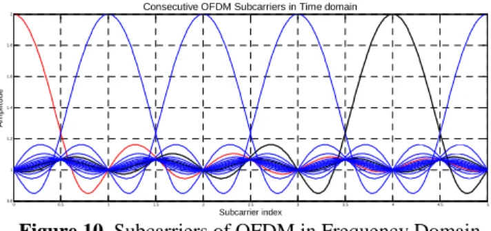
4.4 Transmissions Capacity
In addition to the Spectrum and interference challenges, transmission capacity is another serious concern. Research demonstrates that the transferring data from a UWB based wireless sensor network (to conventional network) is more complex than the regular narrow band wireless networks [45].
0 0.5 1 1.5 2 2.5 3 3.5 4 4.5 5 0.8
1 1.2 1.4 1.6 1.8
2 Consecutive OFDM Subcarriers in Time domain
Subcarrier index
A
m
p
lit
u
d
e
Figure 10. Subcarriers of OFDM in Frequency Domain
4.4.1 Interference Model
For the link capacity understanding, researchers have used several models. Protocol model is the most common and flexible model. We have selected the same pattern for analysis [22].
Let’s assume a signal from node p to q is facing an interference. The region is circular with radius (1+∆) ρpq.
Node p at the center and ρpq is the distance between node p
and q (and ∆ > 0)
Considering the transmission between node p and q is successful (assuming it is not in the interference area of any other active transmission). Now let’s take a physical model here; a signal from p to q is successful if SINR value at receiver node is above the threshold, i.e.
( )
{ } p pq pq
k kq k \ p
P SINR q
N P α
∞
ρ τ
ρ
β
−
−
∈
≅ ≥
+
∑
(7)Pp = power of the pth transmission, τ = parallel transmission
in progress. N=noise power,
And α > 2, and β= Threshold level. On the transmitter side, condition Pp≤ Pind should be followed.
Here the physical model is associated with the decoding process (Signal to Noise Ratio of debugging in multiple modulation patterns) [22]. In simple words, the protocol model is the simplified version of the physical model.
As signal decoding has a direct link with the physical model [22], the protocol model has to be considered as a subset of the physical model.
Using the same scenario with the Gaussian, fading model. The path loss is pq
pq
e−γρ ρ −δ
Here, ρpq is the distance b/w p and q, and γ > 0. As there is
medium absorption, so γ≥ 0 [36]. The output signal at “p” at time t is
( )
( )
( )
( )
pq
q pq p q
p q
y t E e−γρ Q t R t
≠
=
∑
+ (8)Where Qp
( )
t is the impulse by node p, and Rq( )
t is white Gaussian noise with variance σ2p,above ρpq isassumed not less than some ρmin > 0. 4.4.2 Capacity Categories
By assuming a wireless sensor network consists of “n” nodes and fixed (circular) area “A” with nodes’ throughput limitation “w” b/sec. There are two types of capacity matrices that can be considered for the sensor network.
(a) Transmission Capacity (TxC)-(Hierarchical Network)
Supposing, multiple transmission sessions in progress in a given time and space, and the network successfully transports one bit of information for the distance of 1 meter. Here “the sum of products of bits and the distance over which they are carried is a valuable indicator of a network’s transport capacity” [37].
Throughput-(hierarchical network): Considering maximum throughput of multiple connections in the network transmission. The largest communal throughput among links is throughput capacity. Supposing that each node arbitrarily selects a node. Throughput capacity can be defined as the largest communal throughput that can be achieved between any source and destination nodes [38].
The main dissimilarity between two capacity notions is that in the transport capacity for longer distances, more resources are required. So for the (capacity of) data transfer, the distance must be considered (between two points). On the other side, throughput capacity does not consider the distance and all the transmissions are assumed same. Here are the observations.
1st observation: In [39], transmission capacity on “n” nodes is assessed. For the scenario of arbitrary networks Nodes are optimally placed, and traffic patterns are optimally selected. It is observed that by dividing the uniformly among all nodes, each will get Ѳ
(
W / n bit-m/sec. If we go further)
(assuming the same distance of 1m between source and destination), throughput capacity will be Ѳ(
W / n)
bits/sec.2nd observation: As per research by [39] Physical model, though cW n bit-m/sec is achievable, but c Wn′
(
α−1 /)
αBit-m/sec is not.
Precisely 1
2
1 Wn
n 8
6 2
16 2
2
α α α π
β α
+
−
+
−
bit-m/sec is
possible when the network is acceptably designed. Here it is noticed that the higher bound of order Ѳ
(
W / n)
bit-m/sec is possible. In an unusual event (e.g. fraction Pmax/Pmin). The transceivers can be limited by the “β”, in that case, thehigher bound will be 1
1 min
max
8 1
W n
P P
α
π
β −
bit-m/sec.
It is important to understand that, when α has higher value, i.e. signal declines swiftly by distance. These (higher and lower) bounds both limit the transmission capacity.
(b) Transmission Capacity (TxC)-(Arbitrary Networks)
Protocol model: Assuming that nodes “n” are using range “r” in a network infrastructure with the ideal node locations and optimum selection of source/destination. The transmission will be assumed successful if the distance between sender (Xp) and receiver (Xq) node is less than “r” =>
[|Xp-Xq|≤ r]
By assuming that the node Xk uses the same sub-channel, at the same time =>
[|Xk-Xj|≤ (1+∆)r]
Physical Model: Assuming “P” as a power level for all nodes and {Xk; k∈τ} is the subset of nodes which are transmitting
simultaneously on the sub-channel. Transmission between Xp and Xq will be assumed successful if
p q
p q
P
X X
P
N k
X X
α
α
β τ
−
≥ +
−
∑
ò(9)
Throughput (Arbitrary Network): To understand the throughput in a better way, let’s understand the achievable throughput first. “A throughput of λ(n) bits/sec for each node is achievable if there is a spatial and temporal scheme for the scheduling transmission, such that by operating in the network in a multi-hop fashion and buffering at intermediate nodes when awaiting transmission, every node can send λ(n) bits/sec as an average to any selected destination [40].
( )
( )
n
lim Prob(λ n cf n is achieveable 1
→∞ = =
( )
`( )
n
liminf Prob(λ n c f n is acheieveable 1
→∞ = <
Whether a specific throughput is achievable or not, mainly depends on the location. In case of arbitrary network Here c is deterministic constant and C >0 & C’ < +∞ Observations:
The throughput capacity for protocol model will be
( )
Wn
nlogn
λ =Θ
bits/sec pairs and achievable throughput will be bits/sec.
Moreover, for the physical model the achievable throughput will be
( )
cWn )
nlogn
λ = bits/sec.
Implications:
In the above observations an ideal MAC scheduling is assumed. With is no collision during the communication. Similarly, if the value of “n” (number of nodes) is kept large, the throughput will decrease, and that might not be acceptable. Whole analysis are based on static nodes, (without any mobility) that could be another concern. Despite all, energy consumption by participating nodes during data communication is neglected, which needs consideration. Another important observation; when value of
α is large, capacity is good enough for both the cases (throughput and transport).
The author in [41] has explored the transmission limits under UWB by using Gaussian fading model. Considering output results, it is the best capacity analysis work.
Figure 11.Two steps-Analog Synchronization
4.5 Synchronization:
Another challenging area for UWB based sensor network is “Synchronization”. As synchronization has an enormous impact on the network performance, proper synchronization for each link (from point to point and multi-point) is a key requirement. Particularly in a dense network environment where severe inter-symbol interference (ISI) factor exists. For a UWB based communication system, selection of a modulation scheme requires lots of traits, e.g., data rate, channel condition, receiver type, error coding, ISI, and interference factor. Modulation for the UWB is categorized into two main kinds, Single band and Multiband. Here Multiband is in fact division of UWB bandwidth in sub-bands (of course with less bandwidth), and it is known that the band comprises of 3.1-10.6GHz [42]. Different coding techniques are used for the communication through multi-band. Time-frequency code is the common approach for the data sequencing.
Sub-bands can use either of the modulation technique single carrier or multi-carriers. Orthogonal Frequency Division Multiplexing (OFDM) is the most adaptable modulation pattern where multiple carriers orthogonally transmit data. Considering OFDM, multi-path energy pool is one of the vital elements that define the communication range for WSN. In the MB-OFDM technique, transmission takes place orthogonally among sub-bands. The advantage of this technique is to collect multipath energy by solo RF sequence. Its downside is its complex transceiver design. OFDM UWB has already been under consideration for WSN.
4.5.1 Timing Synchronization (under UWB)
Hence, for better performance, the sampling rate needs to be in the Gigahertz range (e.g., for OFDM minimum 500MHz and up to 4GHz in case of Impulse Radio). Apart from this ADC must be able to execute 4-6 bit resolution (so that it can consistently resolve signals from interferences, e.g., narrowband). Here, the challenge is such that the performance of an ADC tends to be power hungry. Therefore, it is not feasible for WSN systems, where energy is a vital concern.
An alternative scheme is to use fewer bits for the sampling. That means reduce the ADC speed. One common approach is to use low-speed ADC for the main part of the signal and use the analog domain for the rest tasks [46].
The main challenge with the analog part is the receiver’s template and timing (for received signal and its path). In a digital implementation, multiple correlators, properly delayed with one another (i.e. by pulse duration) are used for the correlation. One of such architecture was proposed in our earlier study [47].
It was observed that timing acquisition is a very complex task, especially in the UWB WSN systems. Mainly because of the limited transmitted power and high-resolution multi-path scheme. For the consistent timing synchronization, if transmitting power is low, it takes very long search time, whereas a received “Rx” signal (combination of multi-path pulses) produces an output in the multiple stages. All of that makes the process very complex. That makes timing acquisition the main bottleneck for a lightweight receiver design. Exact TOE (Timing offset estimation) is the major requirement for the UWB communication, especially OFDM scheme will not fit if TOE is not correct. Most common technique for such case is the “Clean Template” or sliding correlator (between received and transmitted signal) but it is not an ideal solution for Impulse Radio.
While exploring multiple solutions, research [48]-[53] has some improved results for the IR-UWB WSN synchronization. However, most of these techniques are based on assumptions, e.g., 1) assuming no multipath. 2) no time hopping (TH) codes. 3) known multipath channel. 4) complex and long synchronization time. Our analysis is that Timing with Dirty Templates (TDT) is an ideal scheme for IR-UWB, introduced in [54]-[57]. The basic logic behind this technique is a correlation of received signal with “dirty template”. That is, in fact, pulled out from the received waveforms. Term dirty is used as many unknown factors distort it.
4.5.2 Analog Synchronization:
If we analyze the typical UWB radio signal processing method, the first step is signal detection. Moreover, the identification of symbol-level timing offset is the next. Timing synchronization performs the coherent demodulation. That in fact, enables the system to utilize the bandwidth to its maximum capacity. By using analog synchronization ADC can avoid high sampling rate, but its use for WSN is challenging. Research shows that synchronization at the analog front end is very attractive for the wireless sensor network, mainly due to its energy consumption (by dropping the sampling rate and bit resolution) [58]. Research results
by [58] reveal that this technique has significant advantages when used for WSN.
Figure 12. Energy ratio b/w Rx pulse (UWB) and the LO
In figure 12 Correlation function is used for the energy fraction among Rx Pulse & LO pulse. Here the aim was to minimize the errors related to correlation and control the power ratio (over 70 percent of the overall signal power). Misplacement between Rx and the local oscillator signal LO was required to keep under 25ps. That triggered a complex design restriction for the analog synchronization. One direct method to overcome this challenge is the use of closed loop systems [59]. The author in [59], has proposed a close-loop adaptive filter. Considering Wireless Sensors Network, there are design concerns, e.g., a phase locked loop design under current CMOS technology locks the acquisition time at 100 ns. That is very long for synchronization in Wireless Sensor Network. On the other hand, considering the open-loop scheme. The received signal passes through an analog part; synchronization detects a difference (about 10-15 Nano sec limit) in the time range of the received pulse.
Consecutive recapitulation of the correlated Rx (received signal) and LO (Local Oscillator) and analog delay cell show the open-loop synchronization. However, to apply the analog delay a consecutive shift of received signal is needed. Similarly, the use of delay cells using the (acceptable) accuracy (e.g., 25ps) for the entire probing time will generate attenuation at LO signal. The resulting attenuation will mismatch the correlation output (between the first and last stages). Two steps synchronization is one of the solutions to this problem. Thoroughly explained in [58].
Two-step synchronization is based on coarse and fine tracking parts Figure 13.
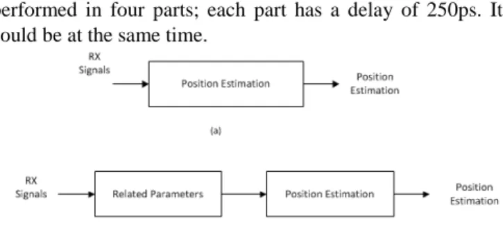
Figure 13. Two-steps analog synchronization scheme [58]
In the coarse gaining, part timing point of Rx (received signal) as per the Tc (chip time) is calculated. The coarse
performed in four parts; each part has a delay of 250ps. It could be at the same time.
Figure 14. WSN-Positioning (direct & 2-way approach)
The signal-probing job is completed by distributing the correlation value of Rx by four equally delayed forms of the template (LO Signal). For each interval correlation value of received signals is compared internally and interval of the highest correlation value is selected. Right after the gaining, synchronizer takes local oscillator signal as input to the fine tracking part. Here at this stage (as showed in Figure 12), the start of Rx (received signal) is synchronized with a Local Oscillator (as per the required time resolution).
Although this fine tracking has to meet several timing chunks, still with its existing status it is very much applicable to WSN applications. Due to this less number of attenuation (that reduces the systems error ratio) Local oscillator’s performance improves significantly. The output from coarse gaining part goes to fine tracking section, which refines the Local oscillator signal according to the timing resolution (e.g., 25ps).
Finally synchronized signal enters the mixer and the signal is correlated with the UWB, and output from correlators goes to ADC [60].
4.6 Position Estimation for WSN
UWB has prodigious features of positioning estimation support, and we know that position estimation is an important requirement of many WSN applications. Categorically WSN positioning (under UWB) could be possible in two ways, “direct approach” and “two-step approach” [77]. In the direct approach, UWB signal is (directly) used, whereas in the two-step signal approach; parameters (extracted from the signal) are used for positioning, and the signal itself does not (directly) involve. Here one concern could be the use of parameters, normally extracted from similar undesired signals. In the direct approach, as the signal individually is involved. Signal’s origin may be verified. The two-step approach has some advantages. It is simple, from a performance point of view it gives same results as direct approach. That makes it more applicable to WSN. Hypothetically position estimation methods are inherently connected to the MAC layer. It consists of schemes for the timing enhancement and related ranging precision. Also, it shares the timing (information) for the exact positioning data, which is a key condition for many UWB-WSN applications and very useful for applications that require position estimation.
By using its own reference time, a network node can easily estimate the time of arrival of a UWB signal from a neighboring node. The reference point is combined with other system measurements for the exact 3D position. Also exchange of clock (timing info) needs collaboration among
nodes. Weak bonding or lack of collaboration of nodes or in other words lack of timing information results in issues, like hidden and expose node problems. Both hidden and expose issues trigger the positioning problem. As a result, the network goes to the unstable state. That can be avoided if media access layer parameters are considered during the design phase of WSN.
At the design phase core areas as MAC support, information sharing, data sampling rate, node scheduling, visibility and signal strength has to be the part of initial wireless sensor network design. Otherwise, post-implementation changes may bring problems. Most common approaches for precise wireless positioning in wireless sensor networks are RSS, TOA, TDOA, and AOA. The author in reference [61] has discussed this in details.
For the positioning errors due to the noise, Kalman filtering is a most common algorithm. This is famous as LQE (Linear Quadratic Estimation), before estimation of variables, multiple in series observations are collected over time. That increases the accuracy of dynamic positioning in sensors networks. Another important aspect of this algorithm is that it does not require too many assumptions. Kalman filtering is discussed in [61].
Another issue for WSN is NLOS (non-line of sight) communication. Which ominously degrades the precision of positioning systems [61]. Therefore, in many NLOS (non-line-of-sight) Wireless Sensor Network, the positioning constraints are much higher than the LOS (line-of-sight) systems. There are numerous methods to overcome this issue. The most common and adaptable method is to detect NLOS data and try to eliminate NLOS errors. A lot of research has been conducted in this direction; Kalman filter is one of the techniques [61]. Which is very attractive for many cases. Another solution was presented by Guvenc in his research paper [61], [62]. This technique has many interesting scenarios. Mainly in this technique detection of NLOS (non-line-of-sight) errors is based on channel attributes.
5.
Current Status and Future
5.1 Possible Target Area/Applications
5.1.1 Low Data Rate (LDR) Applications
energy detection (technique) [63] is a compatible and applicable approach.
Looking at its commercial use, surveillance applications designed on IR-WSN are already on the market, and many militaries and security organizations are using it [64]. IR-UWB’s unique (noise-like) behavior makes it a very feasible platform for the LDR applications. Body area network “BAN” is one of the examples.
5.1.2 High Data Rate (HDR) Applications
UWB is also a good candidate for the high data rate applications. Due to complex structure and communication requirements, high data rate wireless sensor networks require very intricate transceiver architecture. Where size and reliability are two major requirements. OFDM-UWB based wireless sensor platform is the only practical solution that fulfills all these requirements. Currently, researchers are trying to find out a better solution for the jamming issue. It is a major snag in handheld devices under OFDM-UWB. The main focus area of high data rate application includes.
• Multimedia & Interactive Applications
Interactive applications and multimedia-based technologies depend on the very high data rate. These time critical applications sometimes need over 1 Gigabits/second data rate. Similarly some Internet-based services (due to a high number of users) also demand high data rate.
• Smart Devices Interfaces
Due to technology advancement, everybody has multiple gadgets to organize his daily lifestyle. These gadgets use a variety of ways to exchange data. The way the use of sensors is increasing in the SMART technology, the uniform wireless interconnection is greatly in demand to swap the cables and related hardware [65]-[67]. However, such wireless solutions will be attractive for the battery-powered devices without any external power supply.
• Positioning based Applications
Today many SMART applications need an accurate and well-calculated location data. Location data is very critical for many industries and used as pre-requisite for HDR (High data rate) modules. Due to its excellent capabilities UWB is an active approach for the location-based applications.
5.1.3 WBAN (Wireless Body Area Network)
BAN (body area network) is a type of Wireless Sensor Network, which is based on small low-power, smart devices used on the human body to sense different types of measurements. Due to its unique nature it has unique requirements such as,
Heterogeneous: Network structure is complex with many modules, e.g., a sensor unit, actuator node and gateway node. Data rates: Data rate in BAN is usually variable and usually comes in the range of low to medium rates.
Energy: Due to nature of design only low energy consuming platforms work, IR seems an excellent choice for BANs. QOS: BAN is related to medical, so reliability and quality of service are core concerns.
Ultra-wideband based BAN solutions are under considerations and IR, and OFDM both are attractive platforms for BAN.
Besides above, robotics-based industrial requirements, e.g., self-propelled industry, distance and positioning systems and logistic based sensors applications are also attractive candidates for the UWB based sensor networks.
5.2 Future Direction
Due to its remarkable capabilities, ultrawideband short-range sensing solutions are going to be the necessity of everyday life. When this technology is going to be used on a large scale, complex integration (of the multiple sensor networks) could be a major challenge. Another area of concerns is the data processing, execution of sensed data totally depends on the density of application.
Following are a few future directions for UWB based WSN.
• Monitoring public situations, for example, adversities, securing building and areas, climate patterns, and weather forecasting
• Observing habitations, wildlife migration, and population count.
• Home security: use of intelligent robotics.
• Object-ensemble tracking: interpretations of sight by type moreover, by contents [68].
• Nuclear radiation control systems.
• Use in cultivation and irrigation.
• Use for water system is monitoring.
• Distributed video and sensing networks.
• Ground Penetrating Radars (GPR).
• USE in the food industry, e.g., Moisture content, Quality and Life of food.
• Medical industry as remote detection of diseases, e.g., Cancer [69].
• WBAN (Wireless body area network).
• Wireless Multimedia Sensors Networks.
5.3 Open Research Concerns
(a) Effect of UWB on WSN-Network Lifetime
(b) Self-Organizing under UWB
Self-healing is an important need for a sensor network. With a UWB radio layer, it is not easy to adjust the radio transmission range when the topology changes. UWB-Transceiver has to be flexible enough to accept such changes when used in a wireless sensor network. Damage to one link should not disturb the whole network connectivity. That is the basic principle behind all wireless sensor networks. The way in which PHY based on UWB will cope with this challenge is still under research.
(c) Maintenance & change control:
Maintenance for UWB based WSN is considered easy. As far as overall network maintenance is concerned the most common task is the deployment of patches or up gradation of system code (firmware) on each node. All sensor nodes should be updated promptly, with the right version of the code. Maintenance needs to be automated and fully managed. Also, the interruption to the production traffic should be as minimal as possible. Version controlling should be documented. The nodes must have the ability to assess the quality of the link and must be able to indicate any problems that may arise. Each maintenance should be based on a complete implementation plan, back out plan and test plan.
(d) WSN Security and Lifetime under UWB
Security and overall lifetimes of wireless sensor networks are important concerns, which requires continuous attention. Due to the rapid changes in the technology, and WSN’s functional processing capability data integrity is always at risk [78]. Wireless Sensor Network lifetime can be increased by implementing modern zoning technique.
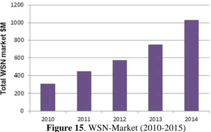
Figure 15. WSN-Market (2010-2015)
Use of UWB for medical, military and other critical applications needs additional carefulness. Radio, Transport, and MAC layer should be design with extra care so the network can tackle the external attacks. Here the main
challenge is data encryption, which requires a large amount of processing power and memory that is why heavy encryption is not encouraged in WSN.
Another concern is integrity of sensed data that in fact is the essence of the whole network; a minor manipulation can trigger a serious loss. So data alteration of any type should strictly be controlled. Similarly, a legitimate broadcast is crucial which can certify the sender and its data. Denial of service is another serious security concern in WSN. That can stop the whole network from their basic function and can be triggered by sleep deprivation agony: energy source may get weaker by nonstop service requirements or need for valid but severe tasks [75].
5.4 Concluding remarks
This survey has presented a detailed overview of ultra-wideband, and it is implications when used in wireless sensor network. UWB in its both forms OFDM and IR is an amazing platform for the wireless sensor network though there are many challenges that need to be resolved. Most of these challenges are related to the spectrum, transmission, synchronization, and coverage. During this survey multiple research resources in the domain of WSN are reviewed, and core concerns were identified with the possible direction of the problem resolution.
Technology trends show that in future, the use of UWB for the sensor applications will increase, and this increase will directly impact the spectrum. In-fact spectrum management is a key requirement for the use of UWB in future sensor networks. Here we have highlighted possible challenges in terms of UWB spectrum utilization and pointed out concerns about its licensing. We have also discussed other issues like connectivity and interference that may create serious communication problems for wireless sensor network. One key problem to resolve, while connecting multiple sensors by UWB radio is the likelihood of joint interference by other radios that already operate in the same 3.1–10.6GHz range. To tackle such issues, we have recommended new techniques for the resolution (e.g., cognitive radio).
In addition to the theoretical analysis here we have also surveyed some existing technology solutions and highlighted their strengths and weaknesses.
References
[1] Wu Ji, Wang Wei, Liang Qilian, Wu Xiaorong, Zhang Boaju, “Compressive sensing-based signal compression and recovery in UWB wireless communication system”, Wireless Communications and Mobile Computing, Vol. 14 Issue 13, pp. 1266-1275, Sep. 2014.
[2] P. Martigne, “UWB for low data rate applications: Technology overview and regulatory aspects”, in Proc. IEEE Int. Symposium. Circuits System (ISCAS), pp. 2425–2428, 2006.
[3] K. D. Colling, P. Ciorciari, “Ultra-wideband communications for sensor networks”, in Proc. IEEE Military Communication Conference (MILCOM), pp. 1–7, 2005.
[4] S. Gezici, Z. Tian, G. B. Giannakis, H. Kobayashi, A. F. Molisch, H. V. Poor, and Z. Sahinoglu, “Localization via ultra-wideband radios: A look at positioning aspects for future sensor networks”, IEEE Signal Process. Magzine., vol. 22, pp. 70–84, 2005.
[5] R. S. Thoma, O. Hirsch, J. Sachs, and R. Zetik, “UWB sensor networks for position location and imaging of objects and environments”, in Proc. 2nd Eur. Conf. Antennas Propagation (EuCAP), pp. 1–9, 2007.
[6] L. Yuheng, L. Chao, Y. He, J. Wu, and Z. Xiong, “A perimeter intrusion detection system using dual-mode wireless sensor networks”, in Proc. 2nd Int. Conference Communication Network. China, pp. 861–865, 2007. [7] X. Huang, E. Dutkiewicz, R. Gandia, and D. Lowe,
“Ultra-wideband technology for video surveillance sensor networks”, in Proc. IEEE Int. Conference Industrial Informatics, pp. 1012–1017, 2006.
[8] J. Li and T. Talty, “Channel characterization for ultra-wideband intra-vehicle sensor networks”, in Proc. Military Communication. Conf. (MILCOM), pp. 1–5, 2006.
[9] F. Granelli, H. Zhang, X. Zhou, and S. Marano, “Research advances in cognitive ultra wideband radio and their application to sensor networks”, Mobile Network Application vol. 11, pp. 487–499, 2006.
[10] L. Stoica, A. Rabbachin, H. O. Repo, T. S. Tiuraniemi, and I. Oppermann, “An ultra-wideband system architecture for tag based wireless sensor networks”, IEEE Trans. Vehicle Technology, vol. 54, pp. 1632–1645, 2005.
[11] I. Oppermann, L. Stoica, A. Rabbachin, Z. Shekby, and J. Haapola, B UWB wireless sensor networks: UWENVA practical example, IEEE Commun. Mag., pp. S27–S32, 2004. [12]Seungryeol Go, Jong-Wha Chong, “Improved TOA-Based
Localization Method with BS Selection Scheme for Wireless Sensor Networks”, ETRI Journal, Vol. 37 Issue 4, p707-716, August 2015.
[13]Author Eugenio Iannone, “Telecommunication Networks Devices, Circuits, and Systems”, Illustrated Edition. CRC Press, ISBN: 1439846367, 9781439846360, pp. 318-319, 2011.
[14] G. Hoblos, M. Staroswiecki, A. Aitouche, “Optimal design of fault tolerant sensor networks”, IEEE International Conference on Control Applications”, pp. 467–472 Sep. 2000. [15]Chunyan Zhang, Sanyang Liu, Zhaohui Zhang, “Design of Efficient Heterogeneous Wireless Sensor Networks based on Small World Concepts”, International Journal of Advancements in Computing Technology, Vol. 7 Issue 4, p1-9, July 2015 .
[16] E. Shih, S. Cho, N. Ickes, R. Min, A. Sinha, A. Wang, A. Chandrakasan, “Physical layer driven protocol and algorithm design for energy-efficient wireless sensor networks”, Proceedings of ACM MobiCom’01, Rome, Italy, pp. 272– 286, July 2001.
[17] M. Chiani, A. Giorgetti, and G. Liva, “Ultra-wide bandwidth communications towards cognitive radio”, in Proc. EMC
Europe Workshop Electromagnetic. Comp. Wireless Systems, Rome, Italy, pp. 114–117, Sep. 2005.
[18]Z. Chunyan, S. Liu, Z. Zhaohui, “Design of Efficient Heterogeneous Wireless Sensor Networks based on Small World Concepts” International Journal of Advancements in Computing Technology; ISSN: 20058039, Vol. 7 Issue 4, pp. 1-July 2015.
[19] Zhuo Li, Qilian Liang, “Capacity Optimization of IR Ultra-wide Band System Under the Coexistence with IEEE 802.11n”, Adhoc & Sensor Wireless Networks, Vol. 21 Issue 1, p59-75, 2014.
[20] Xuemin Shen, Mohsen Guizani, Robert Caiming Qiu, Tho Le-Ngoc, “Ultra-Wideband Wireless Communications and Networks” Publisher John Wiley & Sons, ISBN 0470028513, pp. 8-9, 2007.
[21] Rahman, M. Azizur, Villardi, G. Porto,Lan, Zhou, Baykas, Tuncer, Pyo, Chang-Woo, Song, Chunyi, Sum, Chin-Sean, Wang, Junyi, Harada, Hiroshi, National Institute of Information and Communications Technology (Tokyo, JP), Patent number: 8,929,315. Jan. 2015.
[22] Syan Bingbing, Ren Wenbo, Yin Bolin, Li yang, “An indoor positioning algorithm and its experiment research based on RFID”, International Journal of Smart Sensing & Intelligent Systems, Vol. 7 Issue 2, p879-897, Jun. 2014.
[23] A. F. Molisch, “Ultra-wideband propagation channels-theory, measurement, and modeling”, IEEE Trans. Vehicle. Technology, vol. 54, pp. 1528–1545, Sep. 2005.
[24] Mohamed R. Mahfouz, Aly E. Fathy, Michael J. Kuhn, Yahzou Wang, “Recent Trends and Advances in UWB Positioning”, IEEE MTT-S International Microwave Workshop on Wireless Sensing, Local Positioning, and RFID, Croatia 2009.
[25] IS 2004-31, Intel White Papers, “Ultra-wideband technology, enabling high-speed personal area networks”, http://www.caba.org.
[26] Marco Chiani, “Coexistence between UWB and Narrowband Wireless Communication Systems”. Proceeding of IEEE Vol. 97, No. 2, Feb. 2009.
[27] Ehab M. Shaheen, Mohammed El-Tanany, “Analysis and Mitigation of the Narrowband interference Impact on IR-UWB Communication Systems”, Journal of Electrical and Computer Engineering Volume 2012, Article ID 348982, 2012.
[28] Niels Hadaschick, “Techniques for UWB-OFDM” Institute for Communication Technologies and Embedded Systems, Algorithm Project. WWW.ice.rwth-aachen.de/research. [29] A. Erik, L. Peio, A. Leire, Astrain Javier, V. Jesús, F.
Francisco, “Analysis of Wireless Sensor Network Topology and Estimation of Optimal Network Deployment by Deterministic Radio Channel Characterization”, Sensors , Vol. 15 Issue 2, pp. 3766-3788, February 2015.
[30] S. Haykin, “Cognitive radio: Brain-empowered wireless communications”, IEEE J. Sel. Areas Communication, vol. 23, pp. 201–220, Feb. 2005.
[31]C. Manimegalai, R. Kumar, “Performance Enhancement of Multi Band-OFDM Based Ultra Wideband Systems for WPAN”, Wireless Personal Communications, Vol. 82 Issue 1, p183-200, May 2015.
[32] Alex Chia-Chun Hsu, “Coexistence Mechanisms for Legacy and Next Generation Wireless Networks Protocols”, University of Southern California. Electrical Engineering ProQuest, ISBN: 0549606017, 2007.
![Figure 2. Generic block diagram of a WSN-Node [16]](https://thumb-us.123doks.com/thumbv2/123dok_us/8125656.2155035/3.892.475.809.335.532/figure-generic-block-diagram-wsn-node.webp)
![Figure 8. Normalized Transfer Function [27]](https://thumb-us.123doks.com/thumbv2/123dok_us/8125656.2155035/5.892.464.804.483.709/figure-normalized-transfer-function.webp)
![Figure 9. Frequency Domain representation of OFDM over BFC for a code word [29]](https://thumb-us.123doks.com/thumbv2/123dok_us/8125656.2155035/6.892.464.828.277.541/figure-frequency-domain-representation-ofdm-bfc-code-word.webp)