Bayesian and frequentist methods for approximate inference in generalized linear mixed models

(1)

Bayesian and Frequentist Methods for Approximate Inference in

Generalized Linear Mixed Models

Evangelos A. Evangelou

A dissertation submitted to the faculty of the University of North Carolina at Chapel Hill in partial fulfillment of the requirements for the degree of Doctor of Philosophy in the Department of Statistics and Operations Research (Statistics).

Chapel Hill 2009

Approved by,

Richard L. Smith, Advisor

Zhengyuan Zhu, Advisor

Chuanshu Ji, Committee Member

Bahjat F. Qaqish, Committee Member

(2)

(3)

Abstract

EVANGELOS A. EVANGELOU: Bayesian and Frequentist Methods for Approximate Inference in Generalized Linear Mixed Models

(Under the direction of Richard L. Smith and Zhengyuan Zhu)

Closed form expressions for the likelihood and the predictive density under the Generalized

Linear Mixed Model setting are often nonexistent due to the fact that they involve integration

of a nonlinear function over a high-dimensional space. We derive approximations to those

quantities useful for obtaining results connected with the estimation and prediction from a

Bayesian as well as from a frequentist point of view. Our asymptotic approximations work

under the assumption that the sample size becomes large with a higher rate than the number

of random effects.

The first part of the thesis presents results related to frequentist methodology. We derive

an approximation to the log-likelihood of the parameters which, if maximized, gives estimates

with low mean square error compared to other methods. Similar techniques are used for the

prediction of the random effects where we propose an approximate predictive density from the

Gaussian family of densities. Our simulations show that the predictions obtained using our

method is comparable to other computationally intensive methods. Focus is given toward the

analysis of spatial data where, as an example, the analysis of the rhizoctonia root rot data is

presented.

The second part of the thesis is concerned with the Bayesian prediction of the random effects.

First, an approximation to the Bayesian predictive distribution function is derived which can

be used to obtain prediction intervals for the random effects without the use of Monte Carlo

methods. In addition, given a prior for the covariance parameters of the random effects we

derive approximations to the coverage probability bias and the Kullbak-Leibler divergence of

the predictive distribution constructed using that prior. A simulation study is performed where

we compute these quantities for different priors to select the prior with the smallest coverage

probability bias and Kullbak-Leibler divergence.

(4)

Acknowledgments

I would like to acknowledge particularly my advisors, Richard Smith and Zhengyuan Zhu for

their guidance, advice, and financial support. Special thanks go to all my teachers for providing

(5)

List of Tables

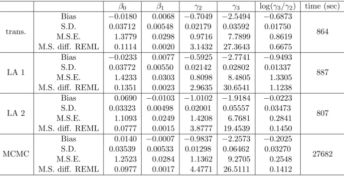
4.1 Simulations for estimation when nugget is known. . . 43

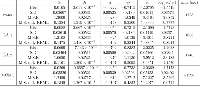
4.2 Simulations for estimation when nugget is unknown. . . 44

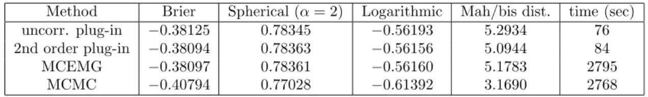
5.1 Measures for comparing different methods for prediction. . . 51

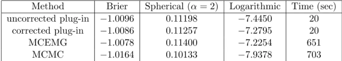
6.1 Measures of scoring for comparison of plug-in and MCEMG. . . 53

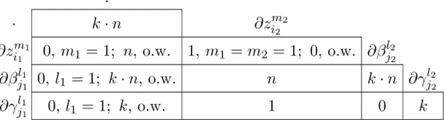
7.1 Derivatives of the joint log-likelihood. . . 57

7.2 Order of magnitude of the derivatives of the log-likelihood. . . 59

7.3 Priors used for the simulations. . . 75

7.4 Approximate coverage probability bias. . . 76

7.5 Comparison of the absolute coverage probability bias. . . 81

7.6 Coverage probability bias computed by simulations. . . 88

7.7 Comparison of the absolute coverage probability bias by simulations. . . 88

7.8 Kullback-Leibler divergence . . . 88

7.9 Proportions for comparing the Kullback-Leibler divergence. . . 92

(8)

List of Figures

1.1 Infected number of roots and total number of roots observed at locations. . . 2

3.1 Connected and unconnected partitions. . . 26

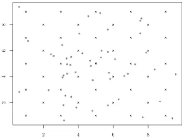
4.1 Observed locations for estimation. . . 41

5.1 Observed locations and locations for prediction. . . 50

6.1 Map of the predicted random effects (disease intensity). . . 53

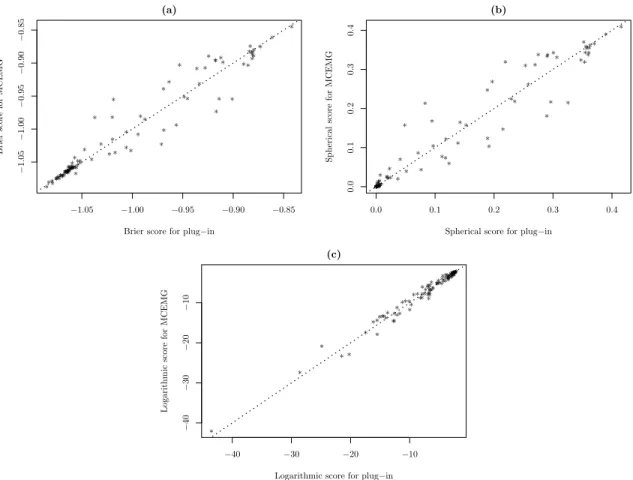
6.2 Calculated scores for plug-in and MCEMG.. . . 54

7.1 Coverage probability bias at the 2.5% and 5% quantiles with range varying.. . . . 82

7.2 Coverage probability bias at the 95% and 97.5% quantiles with range varying. . . . 83

7.3 Coverage probability bias at the 2.5% and 5% quantiles with sill varying. . . 84

7.4 Coverage probability bias at the 95% and 97.5% quantiles with sill varying. . . 85

7.5 Coverage probability bias at the 2.5% and 5% quantiles with nugget varying. . . . 86

7.6 Coverage probability bias at the 95% and 97.5% quantiles with nugget varying. . . 87

7.7 Boxplots of coverage probability bias for 2.5% and 5% quantiles. . . 89

7.8 Boxplots of coverage probability bias for 50% and 95% quantiles. . . 90

7.9 Approximated and simulated coverage probability bias at the 2.5% quantile under priors 1 and 2 against sill . . . 91

7.10 Approximated and simulated coverage probability bias at the 2.5% quantile under priors 3 and 4 against sill . . . 91

(9)

CHAPTER 1

Introduction

A statistical model is a tool for describing random phenomena in terms of mathematical

equations. Although such models rarely manage to capture the phenomenon exactly, they are

still useful in the sense that they provide a way of understanding the phenomenon under study.

Here we focus on a specific model that is general enough to find many applications such as

in medical experiments (ex. 6.2 in Breslow and Clayton, 1993), genetics (ex. 6.6 in Breslow

and Clayton, 1993), environmental sciences (ex. 1 in Diggle et al., 1998), epidemiology (Zhang,

2002) among others.

The Generalized Linear Mixed Model (GLMM) is a type of model that is general enough

to be used for modeling data from discrete as well as continuous distributions and to allow for

different sources of variability in the mean response. The first feature is achieved by specifying

the mean of the response as a function (usually nonlinear) of some explanatory variables. The

second feature is achieved by modeling the mean of the response as a function of random

variables called the random effects.

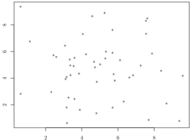
An example

Consider the following example adapted from Zhang (2002). In this example, a plantation

of wheat and barley suffers from a disease called rhizoctonia that attaches to the roots of plants

and hinders the absorption of water and nutrients by them. In order to be able to apply

sufficient treatment to the plantation, we would like to construct a map showing the severity

of the disease in the whole area. To achieve that, a sample of 15 plants where each plant has

multiple roots was collected at 100 different locations and the number of roots and infected

(10)

roots out of the total number of roots observed at each location.

0 200 400 600 800

0 100 200 300 400 500 14/167 21/154 5/127 3/105 38/116 41/166 62/159 45/98 8/164 38/130 9/125 18/115 30/127 5/116 33/114 30/122 28/126 14/170 23/194 12/90 18/144 29/120 15/125 13/132 22/120 17/110 30/167 50/172 9/138 15/128 26/152 27/143 45/133 37/95 12/165 16/105 70/145 21/133 35/145 17/132 26/155 25/102 16/141 11/126 16/178 27/109 37/140 23/140 30/154 30/80 46/152 9/91 36/149 39/128 27/124 13/135 42/113 20/104 27/142 29/154 27/142 9/153 29/145 20/133 46/139 37/160 17/133 31/156 18/121 19/127 40/141 11/184 22/135 12/145 2/147 1/126 5/153 5/116 16/154 14/138 13/125 19/121 17/143 8/152 44/187 21/151 9/144 37/108 25/123 24/116 3/151 42/160 50/165 18/165 35/141 30/1235/143 42/197 22/159 13/166

Figure 1.1: Figure showing the infected number of roots out of the total number of roots observed at the different locations.

The nature of the data does not allow us to model them as continuous variables but instead

they should be modeled as binomial where the probability of observing an infected root is

higher where the disease is more severe. In addition, since the data depend on the locations

that were drawn from, a separate sampling involving data from different locations would result

to a different disease mapping, therefore, the effect of the disease intensity at each location

should be considered random in order to account for the variability due to sampling, hence a

random effect. Furthermore, it is natural to assume that observations at nearby locations are

highly correlated compared to observations from locations that are far apart.

In this example we are interested in estimating any parameters associated with the

prob-ability of an infected root as well as any parameters associated with the correlation structure

of the random effects. Furthermore, a disease map should be constructed by predicting the

random effects associated with the probability of an infection.

Two questions related to Generalized Linear Mixed Models with statistical interest are (i)

(11)

for solving these questions, suitable for each problem. They can be split into two categories,

those that calculate the likelihood and the predictive density by simulations and those that

evaluate those quantities by approximating them. On the one hand, simulation based methods

become very accurate if the simulation is carried to a large size, but that is sometimes too

computationally intensive. On the other hand, approximation methods are faster but the error

of the approximation can be significant if the sample size is not sufficiently large, which makes

these methods biased.

This thesis is focused on results related to asymptotic methods. Approximate techniques

are used to derive an approximation to the likelihood with small error when the sample size

is large. Parameter estimation is then performed by maximizing the proposed approximation.

We compare the proposed method with other methods by simulations and find that it performs

very well compared to the other methods.

The same techniques are used for approximating the predictive likelihood. These lead us

to the definition of an approximate plug-in predictive density which has the Normal density.

Prediction intervals for the random effects are constructed by obtaining the necessary quantiles

of this approximate distribution. This method is also compared to other existing methods and

shows good performance compared to them.

From a Bayesian point of view, estimation and prediction is performed by drawing random

samples from the posterior distributions of the parameters and the random effects given the

sample. We derive a similar approximation to the Bayesian predictive distribution function and

show how our approximation can be used to derive corrections to the Bayesian (and frequentist)

prediction intervals using random sampling. Furthermore, we propose criteria for assessing

the performance of the prior based on approximations to the coverage probability bias and

Kullback-Leibler divergence.

The rest of the thesis is organized as follows. In chapter 2 we review the literature in

Generalized Linear Mixed Models and related topics. The model under study in this thesis

is defined in chapter 3 where we also derive some useful results that will be used later in

the thesis. Chapter 4 deals with issues related to the maximum likelihood estimation and

chapter 5 contains similar results in the case of the predictive density. An example on how

the theory in the previous chapters can be applied is presented in chapter 6. In chapter 7

(12)

we derive approximations to the Bayesian prediction quantiles. We also show how the bias of

the Bayesian predictive density and the Kullabck-Leibler divergence can be approximated and

describe how these quantities can be computed. A comparison of several Bayesian predictive

densities is performed constructed under different priors by comparing the coverage probability

(13)

CHAPTER 2

Background

2.1 Generalized Linear Mixed Models

Statistical models are generally used to explain the variability in the values of one variable,

theresponse, in terms of the values of other variables, thepredictors. From a statistician’s point of view, the challenges of any model fitting are developing a methodology for estimating the

parameters of the model, as well as predicting any unobserved random variables.

The simplest model, and the most widely studied, is theLinear Model. Its main assumptions are that (i) the observations are independent, (ii) the mean equals a linear combination of the

predictors, and (iii) the variance of the response is constant for every observation. An additional

fourth assumption is sometimes made, that (iv) the observations are a sample from the Normal

distribution. Procedures for fitting linear models which are very easy to implement have been

developed. However, the above assumptions are not always satisfied, therefore the use of more

general models is necessary. Such models include theGeneralized Linear Model (GLM) and the

Generalized Linear Mixed Model (GLMM).

The GLM generalizes on the assumptions (ii), (iii), and (iv) above in the following way:

(ii’) a monotone transformation of the mean equals a linear combination of the predictors, (iii’)

the variance is a function of the mean of each observation, and (iv’) the distribution of the

observations is a member of the exponential family. More specifically, suppose that we have

the sample

(14)

which we want to model with respect to a set of covariates

x1,x2, . . . ,xn

Our data consist of a realization of the random variablesY1, . . . Ynwhich according to

assump-tion (iv’), theith variable follows a distribution with probability density/mass function

f(y;θ, ω) = exp[ω−1_{y θ₋b(θ)_}+c(y, ω)] (2.1)

for known functions b and c, and with canonical parameter θ and dispersion parameter ω. Examples of distributions with density/mass function (2.1) are the Normal, Poisson, Binomial,

and Gamma distributions. For certain members of this family of distributions, the dispersion

parameter ω is known and is in general of less importance. The parameter θ on the other

hand, plays an important role, especially because of its relationship with the mean µ of the

distribution by the equation

µ=b0(θ) (2.2)

and needs to be estimated from the data. Furthermore, the variance, as a function of θequals

v(θ) =ω b00(θ) (2.3)

The functionbis called thecumulant function andvis called thevariance function (McCullagh and Nelder, 1999).

A linear combination ηi =xT_iβ of the response is called the linear predictor and according

to assumption (ii’), for some strictly increasing function g, called the link function,

g(µi) =ηi (2.4)

In the special case of the linear model,g is the identity function.

Note that by (2.2) and (2.4), a one-to-one relationship exists between θi and ηi. A natural

choice would be to choose g such that θi = ηi in which case g is called the canonical link

(15)

the matrix with rows xi’s and ythe vector ofyi’s.

The GLMM introduces a further generalization of the linear model by relaxing the

assump-tion (i) that the observaassump-tions are independent and assuming (i’) that they are conditionally independent given an unobserved random variable Zcalled therandom effect. In this case, the linear predictor is written as

ηi =xTiβ+uTiZ (2.5)

for knownui. A usual assumption of the distribution of the random variableZis that is Normal

with mean zero and some varianceΣ=Σ(γ) that is parameterized by an unknown parameter

γ, called the variance components, that is

Z_∼N(0,Σ) (2.6)

In applications, assuming that the correct model is being used, two main questions arise

with statistical interest:

1. How to estimate the parameters β and γ, and

2. how to predict the random effectsZ.

The solution to the first question is related to the notion of the likelihood while the solution to

the second question with the predictive distribution.

2.1.1 Maximum Likelihood Estimation

The most broadly used method for estimation in parametric models is that of maximum

likelihood estimation (MLE) originally proposed by Fisher (1912). The idea is to choose the

value of the parameters that maximizes the joint density of the observations, called the likeli-hood. Under fairly weak regularity conditions the estimate obtained is asymptotically unbiased and asymptotically efficient as the sample size increases.

In linear models, the calculations for deriving the MLE can be done analytically and closed

form expressions for the estimators of the parameters exist. This is not the case for the GLM and

the GLMM so numerical methods are used instead. The MLE for GLM is obtained by applying

(16)

the Iterated Weighted Least Squares algorithm (IWLS) as shown in Nelder and Wedderburn

(1972).

For the GLMM, the log-likelihood of the parameters (β, γ) given the observationsycan be

written (up to a constant), using (2.1) as

`(β, γ_|y) =₋1

2log|Σ(γ)|+ log Z

exp (

X

i

yiθi(β,z)−

X

i

b θi(β,z)−

1 2z

T_Σ−1₍_γ₎_z

) dz

(2.7)

whereθi(β,z) is the expression ofθas a function of (β,z) obtained from (2.2), (2.4), and (2.5).

To understand the difficulties in calculating the MLE let’s consider the simple example

where there is only one random effect z _∼N(0, γ), β is just an intercept term, and for each i,

yi|z∼Po(eβ+z). Then the likelihood of (β, γ) equals

L(β, γ_|y) =eβPyi_e−12logγ

Z exp

zXyi−neβ+z−

1 2γz

2

dz (2.8)

The integral in (2.8) does not have a closed form solution which makes it difficult to calculate

the likelihood accurately. Evaluation of (2.8) is possible using numerical techniques such as

Gauss-Hermite quadrature but as the dimension of z becomes larger, these methods become

unreliable. More advanced methods have been developed for estimation in GLMM. These

include simulation based methods, as in McCulloch (1997) and Booth and Hobert (1999), and

approximation methods as in Breslow and Clayton (1993) and Shun and McCullagh (1995).

Approximate Likelihood

The idea of the approximate methods is to approximate the log-likelihood in (2.7) by

replac-ing the integrand with an approximation of it which can be integrated analytically. Typically

the approximation is performed by applying Taylor expansion to the exponent of the integrand

in (2.7) around the point ˜z that the exponent is maximized. This method of approximating

integrals is known as Laplace approximation (Barndorff-Nielsen and Cox, 1989, sec 3.3). The estimates are then obtained by maximizing the approximate likelihood.

Penalized Quasi Likelihood

(17)

second degree and suggested using an IWLS algorithm for obtaining the MLE. Their method

is outlined below:

Let

ψ(y,z;β, γ) =₋X

i

yiθi+

X

i

b θi

+1

2z

T

Σ−1z (2.9)

i.e. the log-likelihood is `(β, γ_|y) =₋1₂log_|Σ|+ logRexp_{−ψ(y,z;β, γ)_}dz. Let

˜

z = argmin

z

ψ(y,z;β, γ). (2.10)

Note that ˜z is a function of (y;β, γ). Then by Laplace approximation (eq. 4 in Breslow and

Clayton, 1993)

`(β, γ_|y)_{≈ −}1

2log|Σ| − 1

2log|ψzz(y,z˜;β, γ)| −ψ(y,z˜;β, γ) (2.11)

whereψzz(y,z˜;β, γ) denotes the matrix of the second order derivatives ofψwith respect to the

components of z evaluated at ˜z. For fixedγ, Breslow and Clayton (1993) noted that the term

log_|ψzz(y,z˜;β, γ)|varies very little with respect to β, therefore the estimate ofβ is obtained

by maximizing ₋ψ(y,z˜;β, γ), which is of the form of the log-likelihood for GLM. Hence, the

IWLS algorithm which is used for obtaining the MLE ˆβ in GLM can be used for estimating

β. Substituting ˆβ into (2.11) and noting that the profile likelihood for γ has the form of the

likelihood if the data were following a Normal distribution, the estimate ˆγ is obtained by REML.

The obvious procedure to follow is first to set a starting value for γ, estimate β and use ˆβ to

estimate γ. Then ˆγ is used to obtain a new ˆβ which is in turn used to re-estimate γ. These

steps are repeated until the algorithm converges.

From computational point of view, apart from the challenge of finding ˜zwhen its dimension

is large, the algorithms suggested are easy to implement. Breslow and Clayton (1993) provided

several examples that their method applies but they noted that it doesn’t perform well in certain

examples, e.g when used to analyze binary clustered data. Breslow and Lin (1995) and Lin and

Breslow (1996) improved the method of Breslow and Clayton (1993) by including higher order

terms in the Taylor expansion of ψ but even so there are cases where the estimates are highly

biased. This is the case when the dimension of the random effects is comparable with the

(18)

sample size.

Direct Laplace Approximation

Shun and McCullagh (1995) looked at problems where the dimension of the random effects

increases with the sample size. This assumption is necessary for the variance components to

be estimated consistently but under this framework it is not clear if the remainder term in

the classical Laplace approximation is bounded. In their paper Shun and McCullagh derived a

formula that takes this into account by grouping terms according to their asymptotic order, an

application of which can be found in Shun (1997).

More specifically, they noted that a suitable approximation to the log-likelihood in (2.7) is

−ψ˜₋1

2log|Σ| − 1

2log|ψ˜zz|+ 1 8

X

ijkl

˜

ψijklψ˜ijψ˜kl

−1₈ X

ijklmt

˜

ψijkψ˜lmtψ˜ijψ˜klψ˜mt−

1 12

X

ijklmt

˜

ψijkψ˜lmtψ˜ilψ˜jmψ˜kt (2.12)

Here, the subscripts on ψ denote differentiation with respect to the elements of z, the

su-perscripts denote the inverse elements of the Hessian of ψ, ψzz and the tilde means that the

function ψ and its derivatives are evaluated at the ˜z defined in (2.10). In addition, the

in-dices in the summations range over the dimension of z. The expression in (2.12) is maximized

simultaneously over (β, γ) to obtain the corresponding estimates.

It should be noted here that although their method performs well for small sample sizes,

it becomes slow even for moderate samples because it involves the summation of many terms.

In fact, Shun in his application excluded some non-small terms from the likelihood to speed

up the convergence of the algorithm. Later, Noh and Lee (2007) found a way to include these

terms when the design matrix of the random effects has many zeros, which is the case of the

crossed random effects.

Although these approximation methods perform very well in many situations, the estimates

obtained are biased because of the error in the Taylor expansion. Of course the bias can become

smaller by including more terms in the expansion, as in Raudenbush et al. (2000), but on the

(19)

Simulation based methods

The idea behind simulation based methods is to evaluate any integrals that occur by

simu-lating random numbers from an appropriate distribution. Under some regularity conditions, if

X1, . . . , XN is an i.i.d. sequence andh(x) is some function then, by the Law of Large Numbers,

E₍_h₍_X₁₎₎_≈_N−1P_h₍_X_i_).

Note that the log-likelihood in (2.7) can be expressed as E₍_f₍_y_|_Z_{)) where the expectation}

is taken over the distribution of Z which is N(0,Σ). A rather naive method to evaluate this expectation would be to simulate a large number of random effects from (2.6), plug them into

f(y_|z) and then average over the simulations. Unfortunately this simple method fails if the

sample size is large, and that is because the conditional density f(y_|z) would be so small that

is numerically indistinguishable from 0.

Three suggestions were proposed by McCulloch (1997) with the key point of using the

Metropolis-Hastings algorithm to simulate from the distribution ofZ_|y.

Monte Carlo EM

The EM algorithm is an iterative method for maximizing the likelihood in the presence of

latent variables. In each iteration the parameters are chosen such that they maximize the

expec-tation E_(log_f₍_y_,_Z₎_|_y_{) over the distribution of} _Z_|_y _{with parameters taken from the previous}

iteration. The parameters are updated until convergence of the estimates.

In GLMMβ is updated by maximizing

E_(log_f₍_y_|_Z_;_β₎_|_y₎ _(2.13)

and γ is updated by maximizing

E(logf(Z;γ)_|y) (2.14)

Since none of (2.13) or (2.14) can be evaluated analytically, McCulloch (1997) suggests using the

Metropolis-Hastings algorithm to simulate a sample from the distribution of Z_|y and evaluate

the expectations numerically. On the other hand, some testing has to be made on whether the

sample produced is approximately an i.i.d. sample from the target distribution. Alternatively

Booth and Hobert (1999) suggested two other algorithms that don’t require the simulation of

(20)

a Markov Chain, and hence are more efficient than the one proposed by McCulloch.

Monte Carlo Newton-Raphson

In another point of view, instead of trying to maximize the log-likelihood, McCulloch (1997)

proposes estimating the parameters by setting the scores equal to 0. In this case, an estimate

forβ is obtained by solving

E

∂

∂βlogf(y|Z;β)

y

= 0 (2.15)

and for γ by solving

E

∂

∂γ logf(Z;γ)

y

= 0 (2.16)

The left hand side of (2.16) has an analytical expression and it can be solved easily. On the other

hand (2.15) is not so easy to solve but it is evaluated numerically using the same algorithms as

with the Monte Carlo EM case.

Simulated Maximum Likelihood

The idea of Simulated Maximum Likelihood is as follows. Suppose there exists a random

variableZ∗ with density functionf∗such that f∗(z;β, γ)>0 wheneverf(z_|y;β, γ) >0. Then

the log-likelihood can be written as

`(β, γ_|y) = logE

f(y,Z∗;β, γ)

f∗₍_Z∗_;_{β, γ}₎

(2.17)

where the expectation is taken over the distribution ofZ∗. The expectation is then calculated

numerically by simulating from the distribution of Z∗ and averaging. We noted earlier that

evaluating the log-likelihood by naive Monte Carlo integration is not possible but here if f∗ is

chosen appropriately then the simulated likelihood should be possible to evaluate. (In fact, the

best choice forf∗₍_z_{) is} _f₍_z_|_y_{).) To this end, McCulloch (1997) did not give a clear answer as}

to what to choose for f∗ _{and in his example he chose} _f∗₍_z_;_{β, γ}_{) =} _f₍_z_;_γ_{) which is of course}

unknown, but even in this case his method did not perform as well as the MCEM or MCNR

(21)

2.1.2 Prediction

We now review methods for predicting the random effects themselves or other random

variables that are correlated with them such that conditioned on the random effects, they are

independent on the observations. We use the symbolZ0 for the variable that we want to predict

given a sampleY.

Best Prediction

The best prediction for the random variableZ0is defined as the random variable ˆZ0= ˆZ0(Y)

such that the mean square prediction error E_{_{( ˆ}_Z₀ ₋_Z₀₎2_} _{is minimized. This reduces to}

ˆ

Z0 = E(Z0|Y) which also depends on the parameters of the model. If the parameters were

known, the best predictor can be calculated either by using the Metropolis-Hastings algorithm

as was proposed by McCulloch (1997) or any of the two sampling methods of Booth and Hobert

(1999), or approximate the expectation using Laplace approximation (see Vidoni, 2006, for the

case of independent random effects). Of course, in most applications the parameters are not

known. A way to overcome this problem is to replace them with a good estimate, obtained using

one of the methods described in the previous section. This is known as the plug-in approach.

Plug-in approach

A method for obtaining prediction intervals is by constructing thepredictive density, that is the conditional density of the variable we want to predict given the observations: f(z0|y;β, γ).

It can be expressed as

f(z0|y;β, γ) =

R

f(z_R0|z;γ)f(y|z;β)f(z;γ) dz

f(y_|z;β)f(z;γ) dz (2.18)

Similarly, the predictive distribution function is written as

F(z0|y;β, γ) =

R

F(z_R0|z;γ)f(y|z;β)f(z;γ) dz

f(y_|z;β)f(z;γ) dz (2.19)

As we mentioned earlier, (2.18) and (2.19) depend on the parameters which are unknown. The

plug-in predictive density is constructed by replacing the parameters with their estimates based on the sampleyand is a rather simple to construct but on the other hand it has been criticized

(22)

as failing to take into account the uncertainty in estimating the parameters and assumes that

they are the true values.

Barndorff-Nielsen and Cox (1996) made some suggestions on correcting the plug-in

ap-proach, although these have not been applied to GLMM. They considered the fact that the

plug-in and the true predictive distribution are related asymptotically by

F(z0|y; ˆβ,γˆ) =F(z0|y;β, γ) +k−1D(z0|y;β, γ) +O(k−3/2) (2.20)

ask_{→ ∞} wherekis some constant related with the sample size andD is a known expression.

Let zα be the quantiles obtained by inverting the true predictive distribution and ˆzα be the

quantiles obtained by inverting the plug-in predictive distribution. Their first suggestion was to

estimatezαby ˆzα1 whereα1=α−k −1_D_(ˆ_z

α|y; ˆβ,γˆ) in which caseF(ˆzα1|y; ˆβ,γˆ) =α+O(k −3/2₎

instead of O(k−1_{) that would have been if we used just ˆ}_z

α. We should note though, that if

the correction is too large, then α1 might not be between 0 and 1. Their second suggestion

corrects ˆzα directly by using ˆzα −k−1D_f_(ˆ(ˆ_zzα|y; ˆβ,ˆγ)

α|y; ˆβ,γˆ) as an estimator for zα which doesn’t have

the disadvantage of the first method and gives the same order of accuracy. Furthermore, they

derived an approximation to the predictive density of order O(k−3/2) given by

f(z0|y;β, γ) = (1 + ˆr0(z0))f(z0+ ˆr(z0)|y; ˆβ,ˆγ) (2.21)

where ˆr(z0) =D(z0|y; ˆβ,γˆ)/f(z0|y;β, γ) and ˆr0(z0) = (d/dz0)ˆr(z0).

2.1.3 Bayesian solution

We describe the Bayesian approaches to GLMM in a different section since from the Bayesian

point of view, there is no distinction between estimation and prediction.

A major concern regarding Bayesian analysis is the choice of prior distribution for the

parameters. On this subject, we note the papers by Zeger and Karim (1991) where they discuss

Gibbs sampling in longitudinal GLMM, Karim and Zeger (1992) for similar ideas in crossed

random effects models, Berger et al. (2001) and Diggle et al. (1998) discuss prior selection in

(23)

general setting.

Bayesian Monte Carlo Methods

After the prior is selected, say β _∼ π(β) and independently γ _∼ π(γ), one proceeds by

calculating confidence regions from the posterior distributionsπ(β_|y),π(γ_|y), andf(z0|y). The

Monte Carlo methods proceed by constructing the conditional distributionsπ(β_|y,z), π(γ_|z),

f(z_|y, β, γ), andf(z0|z, γ). As in general, these conditional distributions cannot be obtained

analytically (besidesf(z0|z, γ) which is Normal), Markov Chain Monte Carlo techniques, such

as Gibbs sampler and Metropolis-Hastings, are used to simulate from them which sometimes can

be burdensome (see Clayton, 1996). In a recent paper, Fan et al. (2008) proposed a Sequential

Monte Carlo algorithm for simulating from the posterior distributions which is faster than

MCMC, though it does not completely avoid the simulation of Markov Chains.

Integrated Nested Laplace Approximation

Alternatively, Rue et al. (2009), suggest a new methodology based on Laplace

approxima-tion. Writing θ= (β, γ), they express the posterior as

π(θ_|y)_∝ f(y,z;θ)π(θ)

f(z_|y;θ) (2.22)

and the Bayesian predictive density as

f(z_|y) = Z

f(z_|y;θ)π(θ_|y) dθ (2.23)

The idea is to replace the denominator of (2.22) with its Normal approximation using first

order Laplace approximation, centered around the point ˆz = argmax_zf(y,z;θ). Denoting the

aforementioned approximation by ˜fG(z|y;θ) define

˜

π(θ_|y)_∝ f(y,zˆ;θ)π(θ) ˜

fG( ˆz|y;θ)

(2.24)

Equation (2.24) is an approximation to the posterior of θ which can be used to substitute the

second term of the integrand in (2.23). The first term of the integrand is also computed by a

separate application of Laplace approximation. Finally, the integration in (2.23) is performed

(24)

numerically by Gauss-Hermite quadrature.

This approach provides a quick and accurate way of obtaining approximations to the

con-ditional distributions of interest and therefore obtain accurate predictions to the parameters

and the random effects. On the other hand, the computational advantages of this method

are in effect when the inverse covariance matrix of f(z_|γ) is sparse and when the number of

parameters is small.

Bayesian Predictive Distribution Function

In analogy to the plug-in predictive distribution, we note here the Bayesian predictive

distribution function

F(z0|y) =

RRR

F(z0|z;γ)f(y|z;β)f(z;γ)π(β)π(γ) dzdβdγ

RRR

f(y_|z;β)f(z;γ)π(β)π(γ) dzdβdγ (2.25)

Several authors have argued for the Bayesian predictive distribution against the plug-in one in

the sense that it naturally takes into account the uncertainty in the parameters by assigning

the prior distribution (see Geisser, 1993), nevertheless this should not always be conceded as

Smith (1999) mentions examples where the plug-in predictive density performs better.

2.2 Modeling Geostatistical Data with GLMM

In this section we review methods for analyzing geostatistical data, that is, correlated data

observed over a continuous spatial domainS_{whose correlation arises through their dependence}

on an unobserved spatial process _Z = _{Z(s), s _∈ S_}_{. (}_s _{here is an index representing the}

individual elements ofS_{.) In practice, only a finite sample}_Y₁_{, . . . , Y}_n _{is observed corresponding}

to the sampling sites s1, . . . , sn and the objective is to predict the spatial process Z over the

whole domain S_{. In practice this is done by predicting}_Z₍_s_{) on a fine grid that covers} S_.

2.2.1 Gaussian Random Fields

A Random Field over the spatial domain S _{is a process} _Z ₌ _{_Z₍_{s, ω}₎_{, s} _∈ S_{, ω} _∈_Ω_} _such that for fixed s, Z(s, ω) is a random variable on a probability space, say (Ω,_A,Pr) while for

(25)

The mean µ(s) and covariance c(s, s0) of the random field _Z are defined on S _and S2

respectively in the following way

µ(s) = Z

Ω

Z(s, ω) d Pr(ω) (2.26)

c(s, s0) = Z

Ω{

Z(s, ω)₋µ(s)_}{Z(s0, ω)₋µ(s0)_}d Pr(ω) (2.27)

For simplicity, hereafter, we will avoid writing explicitly the second argument ω when we

describe Random Fields.

Note that the definitions in (2.26) and (2.27) can be written asµ(s) =E₍_Z₍_s_{)) and}_c₍_{s, s}0_{) =}

Cov(Z(s), Z(s0))

Homogeneous Gaussian Random Field

In this section, we present a class of Random Fields, theisotropic Gaussian Random Field, that is usually assumed in order to assist with the inference regarding the probability measure

Pr.

The random field_Z(s) with meanµ(s) and covariance c(s, s0_{) is called}_{weakly stationary} _if

for all s, s0 _∈_S _{the following three conditions hold:}

1. E₍_Z₍_s_{)) =}E₍_Z₍_s0_)),

2. Cov(Z(s), Z(s))<_∞, and

3. Cov(Z(s), Z(s0)) can be expressed as a function of s₋s0.

A weaker form of stationarity is a process that is intrinsically stationary defined by replacing condition 3 above by

3’. Var(Z(s)₋Z(s0_{)) can be expressed as a function of}_s₋_s0_.

If in addition to 1, 2 and 3’, the following condition holds

4. Var(Z(s)₋Z(s0_{)) can be expressed as a function of}_k_s₋_s0_k_.

then the process is calledisotropic. If all conditions 1, 2, 3, and 4 hold then the process is called

homogeneous.

(26)

A Gaussian Random Field is the Random Field _Z onS_{where for every subset}_{_s₁_{, . . . , s}_k_} of S_{, the joint distribution of (}_Z₍_s₁₎_{, . . . , Z}₍_s_k_{)) is Gaussian. In connection with the previous}

definitions the distribution of a homogeneous Gaussian Random Field is characterized by its

mean µ, which without loss of generality we will assume that µ = 0, and by its covariance

functionc(dii0) =c(s_i, s_i0) whered_ii0 =ks_i−s_i0k.

Intuitively, the probability measure underlining a stationary Gaussian Random Field is

invariant under parallel transition of the co-ordinate system while for an isotropic Random

Field it is invariant under rotations of the co-ordinate system.

Here we only consider zero-mean homogeneous Gaussian Random Fields.

Covariance Structure

A common practice is to assume that the covariance function c(_·) is parameterized by a few

parameters γ that have a reasonable interpretation regarding the structure of the covariance

between two sampling sites. Some forms of the covariance function c(_·) are

1. Exponential:

c(d) =       

γ1+γ2, ifd= 0

γ2exp{−d/γ3}, ifd >0

(2.28)

2. Gaussian

c(d) =       

γ1+γ2, ifd= 0

γ2exp{−(d/γ3)2}, ifd >0

(2.29)

3. Spherical:

c(d) =               

γ1+γ2, ifd= 0

γ2{1−1.5(d/γ3) + 0.5(d/γ3)3}, if 0< d < γ3

0, ifd_≥γ3

(2.30)

4. Mat´ern:

c(d) =       

γ1+γ2, if d= 0

γ2

Γ(ν) 2ν−1

2√ν d

γ3

ν

Kν(2√ν d/γ3) if d >0

(27)

γ1 is called the nugget and is interpreted as the variability due to measurement error and

microscale variation (i.e. the part of the variation that cannot be estimated because there are no

two sampling sites close enough to indicate it). γ2 is called thepartial sill and is interpreted as

the variance of the random field if there was no nugget. γ3 is called therange and is interpreted

as the distance at which the correlation function reaches 0 for the spherical form, or 5% of

the partial sill for the other forms. In (2.31), ν is called the smoothness parameter and _Kν

corresponds to the modified Bessel function of the second kind of order ν (Abramowitz and

Stegun, 1964).

The Gaussian Geostatistical Model

Suppose a Gaussian Random Field_Z onS_{. In practice, we sample at}_s₁_{, . . . , s}_k_{and observe}

Y = (Y1, . . . , Yk) whose mean is affected by a set of covariates X. For simplicity, let Z =

(Z1, . . . , Zk), Zi = Z(si), i = 1, . . . , k so that Z ∼ Nk(0,Σ) where the (i, i0) element of Σ is

c(_ksi−si0k), parameterized by γ.

The simplest type of relationship we can have between the observations and the covariates

is to express the mean of Y as a linear combination of the covariates:

Y =Xβ+Z (2.32)

The model in (2.32) implies that the distribution of Y is k-dimensional Gaussian with mean

Xβ and covariance matrixΣand in this case estimation ofβ and γ can be performed by either weighted least squares, maximum likelihood, or restricted maximum likelihood.

Several tools under the namekriging have been developed for predicting the random variable

Z0associated with the sampling sites0under the model (2.32). The original work on this subject

was done by Krige (1951) and later developed by Matheron in a series of papers and books (e.g.

Matheron, 1962, 1963). For a collection of these methods see Cressie (1993).

2.2.2 Spatial GLMM

In many applications, for example when the observations involve counts, the Gaussian

Geo-statistical model (2.32) is not appropriate. Diggle et al. (1998) extended the Gaussian

(28)

tistical model to include parametric families depending only on the mean of the spatial process

in the same way that the classical linear model is extended to the generalized linear mixed

model. In other words they define the linear predictor by

η=Xβ+Z (2.33)

and they assumed that the conditional distribution of the observationsY given the random field

Z is a member of the exponential family as defined in (2.1). In addition, all the assumptions

regarding GLMM also hold for the spatial GLMM and as a consequence, all methods that have

been developed for the analysis of GLMM can also be used for this model. Here we present a

few from the literature.

Bayesian MCMC

As we mentioned earlier, when we want to predict the random effect Z0 under GLMM, the

Bayesian approach has the advantage that it incorporates the unknowing of the parameters

into the prior. In their paper Diggle et al. (1998) assigned independent uniform priors with

bounded support for the components of β and γ and used Metropolis-Hastings to simulate

from the posterior distribution ofγ while random samples from the posteriors ofβ andZ0 were

obtained by simulating from the normal distribution. Later on, Christensen et al. (2000) and

Christensen and Waagepetersen (2002) commented on the use of Langevin-Hastings algorithm

for the MCMC simulation as it leads to better convergence and mixing properties than the

Metropolis-Hastings algorithm. They also suggested the use of non-informative flat priors for

the components of β and non-informative inverse Gamma for the partial sill γ2. For the range

parameterγ3, the use of improper prior results to improper posterior, hence they used uniform

proper prior in the first paper and exponential prior in the second. The estimation of the nugget

γ1 was not considered.

Monte Carlo EM Gradient

In connection with the MCEM idea of McCulloch (1997), Zhang (2002) uses a

Metropolis-Hastings algorithm to simulate from the distribution of Z_|y and calculate the expectations

(2.13) and (2.14) needed for the E step but instead of maximizing those expectations at the

(29)

maximization of the expectations which can be cumbersome. For prediction, he noted that the

best predictor is expressed in terms of the expectations of the random effects at the sampling

sites conditioned on the observations, i.e.

E₍_Z₀_|_y_{) =}

k

X

i=1

wiE(Zi|y) (2.34)

where the vector of wi’s,w=cTΣ−1,c= Cov(Z, Z₀). Therefore, after the covariance parame-ters are estimated, the best predictor forZ0 is obtained by evaluating (2.34) for each iteration

of Z_|y and then averaging over all simulations.

Simulated Maximum Likelihood

Christensen (2004) demonstrated the use of Simulated MLE for the spatial GLMM. He

wrote the likelihood function in the form of (2.17) and used simulation to approximate it. As

we mentioned earlier, the best choice for f∗ is f(z_|y;β, γ) which depends on the unknown

parameters. For this reason the author suggested simulating fromf(z_|y;β0, γ0) for some fixed

values (β0, γ0) which are believed to be close to the true ones and which are updated after a

few iterations.

2.3 Contribution of the thesis

This thesis contributes on topics related to Bayesian and frequentist methods for the analysis

of Generalized Linear Mixed Models. The basic idea is to use asymptotic expansions to compute

quantities of interest such as the likelihood or the predictive density. A key role is played by

Laplace approximation, a method for approximating integrals, where an approximation of this

type, suitable for our case, is derived. The particular feature of our approximation is that

it allows the dimension of the variable that is integrated to increase to infinity, a necessary

assumption for estimation and prediction for these models.

For parameter estimation, we propose an approximate likelihood method. There are several

advantages when estimating the parameters this way. First, as our simulations show, the

estimates obtained have low bias and mean square error and second, our method is fast to

compute. Some details are also given on correcting the bias of the approximation.

(30)

We also suggest an approximate prediction method based on the same idea. We apply a

high order approximation to the predictive density and replace the unknown parameters with

their estimates, what is known as the plug-in approach. The proposed density belongs to the

Gaussian family and prediction intervals can be easily computed. We present a simulation study

where we compare our method with other approximate and simulation based methods and show

that our method has similar performance with the other methods with less computation time.

From Bayesian perspective, we investigate the issue of prior selection. We derive

approxima-tions to the coverage probability bias and Kullback-Leibler divergence of the Bayesian predictive

density constructed under different priors. These are computed for different simulations and

for possible choices for priors that are found in the literature. We make selection based on the

criterion of minimum coverage probability bias and minimum Kullback-Leibler divergence. Our

approximation to the coverage probability bias agrees mostly to the one obtained by simulations

but has smaller variation. We find that the best choices are uniform priors for the nugget and

range parameter while for the partial sill we recommend either uniform prior or inverse gamma.

Using exponential prior for the range, results to higher coverage probability bias unless the true

(31)

CHAPTER 3

General Results

3.1 Model and Notation

Throughout this document we use indices to denote components, derivatives and

summa-tions. For the last purpose, any index that appears in an expression as a subscript and as

a superscript, a summation over all possible values of that index is implicit. For this reason

we will denote the components of a vector sometimes by subscripts and sometimes by

super-scripts. For example, the components of the three dimensional vector x will be written as

x1, x2 and x3 or as x1, x2 and x3 depending on the expression i.e. xixi = xixi =P3_i₌₁(xi)2

but xi_xi _{is the square of the} _i_{th element of} _x_{: (}_x

i)2. The (i, j) component of a matrix A

will be written as aij and its inverse (when exists) will have componentsaij. It is also

conve-nient to enclose any set of indices within square brackets to denote the sum over all partitions

of those indices of the products of the corresponding arrays and a number withing square

brackets to denote the different permutations of indices for the corresponding partition, i.e.

x[ijk]=xijk+ [3]xijxk+xixjxk=xijk+xijxk+xikxj+xjkxi+xixjxk.

For any real function f(x), x _∈ Rk_{, its derivative with respect to the} _ith _{component of}

x is denoted by a subscript i.e. fi(x) := ∂f_∂x(x_i) and fij(x) := ∂

2

f(x)

∂xi∂xj. Furthermore, fx is the

gradient of f and fxx is the Hessian matrix. Based on our notation on matrix inversion, fij

is the (i, j) element of f−1

xx: the inverse of the Hessian matrix. Finally, when we refer to the

probability density/mass function of a random variable, we will use the generic symbol f(_·;_·)

with the random variables written at the left of the semicolon and the parameters at the right,

i.e. f(x;θ) is the density/mass ofX depending on parameterθ andf(x_|y;θ) is the conditional

(32)

function. An exception will be made when the distribution is Gaussian, in which case we will

use the letters φand Φ for the pdf and cdf respectively.

The vector of the response variable is denoted by Y with components _{Yili= 1, . . . , k, l =

1, . . . , ni} repeatedly sampled at k different locations within a spatial domain S. We assume

the existence of an unobserved homogeneous Gaussian random field _Z over the whole spatial

region S _{such that conditioned on} _Z _{the observations are independent. We denote by} _Z _the

k-dimensional vector that consists of the components of_Z that correspond to the sampled sites

and we refer to it as the random effects. Furthermore, the meanµi =E(Yil|Zi) =b(θi) for some

known differentiable functionb, called the cumulant function, such thatb0 _{is strictly increasing,}

and variance vi(µi) where vi is a known function called the variance function (McCullagh

and Nelder, 1999). The parameterθi relates to the linear predictorηi=xTiβ+Zi through the

relationshipµi =b(θi) =g−1(ηi) for some functiongcalled the link function. In our asymptotic

analysis we consider the case in which k and ni increase to infinity with the ni’s having the

same order, min_{ni}=O(n) butkis increasing in a lower rate, k/n→0.

We assume that the joint distribution of the random field _Z is Normal with mean 0 and

covariance matrix parameterized by γ, i.e. for the random effects Z we have,

Z_∼Nk(0,Σ(γ)) (3.1)

Conditioned onZ, the density ofY has the form

f(y_|z;β) = exp

( _k

X

i=1

yi(xTiβ+zi)− k

X

i=1

nib(xTiβ+zi) + k

X

i=1 c(yi)

)

(3.2)

for known functions b and c, where yi = Pnj=1i yij. Note that the form of the density implies

conditional independence among the observations given the corresponding random effects.

Al-though in (3.2) we implicitly used the canonical link for the distribution of y, the results that

follow don’t necessarily require this restriction.

We are interested in estimating the parameters (β, γ) of the model as well as predicting a

(33)

Under our model, the likelihood for the parameters is

`(β, γ;y) = Z

f(y_|z;β)φ(z;γ) dz (3.3)

which does not have an analytic expression. In addition, writing the distribution function of

Z0|Z as

Φ(z0|z;γ) = Φ

z0−µ τ

(3.4)

where Φ(_·) denotes the standard normal distribution function and

µ=cTΣ−1z (3.5)

τ2=σ2₀₋cTΣ−1c (3.6)

σ₀2= Var(Z0) (3.7)

c= Cov(Z, Z₀) (3.8)

the predictive distribution function forZ0 given the dataY is

F(z0|y;β, γ) =

R

Φ(z_R0|z;γ)f(y|z;β)φ(z;γ) dz

f(y_|z;β)φ(z;γ) dz (3.9)

Similarly, the predictive density is written as

f(z0|y;β, γ) =

R

φ(z0|z;γ)f(y|z;β)φ(z;γ) dz

R

f(y_|z;β)φ(z;γ) dz (3.10)

Neither (3.9) nor (3.10) have an analytic expression and hence exact prediction intervals cannot

be calculated exactly.

Before we reach the point of proposing methods for obtaining maximum likelihood estimates

and prediction intervals, we derive a formula that allows us to approximate the likelihood and

the predictive likelihood when the sample size is large.

(34)

3.2 Asymptotic Expansions of Integrals

3.2.1 Modified Laplace approximation

Shun and McCullagh (1995) proposed a modification of Laplace’s approximation that can

be used for evaluating integrals of the form

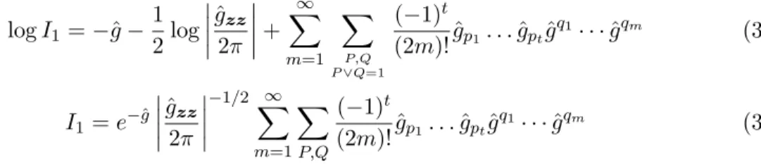
I1 =

Z

e−g(z)dz (3.11)

where g=O(n). Assuming thatg has a unique minimum at ˆz, Shun and McCullagh suggest

an expansion of the integral around that minimum. They derive the identities

logI1 =−ˆg−

1 2log

ˆg₂zz_π

+

∞

X

m=1

X

P,Q P∨Q=1

(₋1)t

(2m)!gˆp1. . .ˆgptˆg

q1

· · ·gˆqm _(3.12)

I1 =e−ˆg

ˆ

gzz

2π

−1/2 _X∞

m=1

X

P,Q

(₋1)t

(2m)!gˆp1. . .gˆptgˆ

q1

· · ·ˆgqm _(3.13)

where the second sum in each of (3.12) and (3.13) is over all partitions P, Q such that P =

p1|. . .|pt is a partition of 2mindices into tblocks, each of size 3 or more and Q=q1|. . .|qm is

a partition of the same indices into m blocks, each of size 2. P _∨Q= 1 means that the union

of the graphs produced by joining elements in the same block of the two partitions is connected

The summation over all the possible values of the 2m indices is also implicit.

i1

i2

i3

i4

i1

i2

i3

i4

Figure 3.1: Connected partitionsQand P1 (left) and unconnected Qand P2 (right)

These formulae require expressing the integrand in a fully exponential form while for the

(35)

In our approach, we consider the following integral:

I2 =

Z

exp_{−g(z)_{} ×}f(z) dz (3.14)

where f is not necessarily positive. Suppose that z _∈ Rk_, _g₍_z_{) =} _O₍_n_{) has a minimum at} ₀

and f and its derivatives areo(n). We will develop a formula for the approximation of (3.14).

Taylor expansion of garound 0 gives

g(z) = ˆg+ 1 2!z

i1_zi2_g_ˆ

i1i2+

1 3!z

i1_zi2_zi3_ˆ_g

i1i2i3 +

1 4!z

i1_zi2_zi3_zi4_ˆ_g

i1i2i3i4+. . . (3.15)

where the subscripts underg imply differentiation with respect to the indicated component of

z and the hats imply that the function or its derivatives are evaluated at 0. The indices range

from 1 tokand the sums are over all indices. Let ˆgzzdenote the hessian matrix of gevaluated

at 0.

A similar expansion of f around the same point gives

f(z) = ˆf + ˆfj1z

j1 ₊1

2fˆj1j2z

j1_zj2₊_{. . .} _(3.16)

Thus

I2 =e−ˆg

Z

e−12zTˆgz zzexp

−_3!1ˆgi1i2i3z

i1_zi2_zi3

−_4!1gˆi1i2i3i4z

i1_zi2_zi3_zi4

−. . .

×

ˆ

f+ ˆfj1z

j1₊1

2fˆj1j2z

j1_zj2₊_{. . .}

dz

=e−ˆg

Z

e−12zTˆgz zz

1₋ 1

3!gˆ[i1i2i3]z

i1_zi2_zi3

− 1

4!ˆg[i1i2i3i4]z

i1_zi2_zi3_zi4

−. . .

×

ˆ

f+ ˆfj1z

j1₊1

2fˆj1j2z

j1_zj2₊_{. . .}

dz

=e−ˆg

ˆ gzz 2π

−1/2

E

1₋ 1

3!gˆ[i1i2i3]Z

i1_Zi2_Zi3

−_4!1ˆg_[_i1i2i3i4]Z

i1_Zi2_Zi3_Zi4

−. . .

×

ˆ

f+ ˆfj1Z

j1 ₊1

2fˆj1j2Z

j1_Zj2₊_{. . .}

whereZ is a normally distributed random variable with mean0 and covariance matrix ˆg_zz−1.

(36)

Then,

I2 =e−ˆg

ˆg₂zz_π

−1/2 _X

r∈{0,3,4,...} ∞

X

s=0

(₋1)r 1

r!s!ˆg[i1...ir]fˆj1...jsE

Zi1

· · ·Zir

·Zj1

· · ·Zjs

where we make the convention if r = 0 then ˆg[i1...ir] = 1, if s = 0 then ˆfj1...js = ˆf and if

r=s= 0 thenE_Zi1

· · ·Zir_·_Zj1

· · ·Zjs_{= 1}

Using equation (2.8) from McCullagh (1987), I2 becomes

I2 =e−ˆg

ˆ gzz 2π

−1/2 _X∞

m=0 2m X s=0 X P,Q

(₋1)t

(2m)!fˆj1...jsgˆp1. . .gˆptgˆ

q1_{· · ·}_ˆ_gqm _(3.17)

whereP is a partition of 2m₋sindices intotblocks each of size 3 or more andQis a partition

of the same indices together with _{j1, . . . , js} intom blocks of size 2. It is not required for P

and Qto be connected.

In the special case wheref(z)>0, say f(z) = exp_{h(z)_}, then from (3.17),

logI2 =−ˆg+ ˆh−

1 2log

₂1_πˆgzz

+ ∞ X m=1 1 (2m)!

X

P,Q P∨Q=1

χp1. . . χpt·gˆ

q1_{. . .}_g_ˆqm _(3.18)

where

χi1···is =

       ˆ

hi1···is ifs≤2

ˆ

hi1···is−gˆi1···is ifs≥3

3.2.2 Approximation to the ratio of two integrals

In the following sections we will need to approximate ratios of integrals e.g. when we want

to approximate conditional densities. Suppose we want to approximate

I2 I1

= R

exp_{−g(z)_{} ×}f(z) dz R

e−g(z)_d_z (3.19)

Using equations (3.13) and (3.17)

I2 I1

=

P∞

m=1

P2m

s=0

P

P,Q

(−1)t

(2m)!fˆj1...jsgˆp1. . .ˆgptˆgq

1_{· · ·}_g_ˆqm

P∞

m=1

P

P,Q

(−1)t

(37)

= ∞ X m=1 2m X s=1 X P,Q

(₋1)t

(2m)!fˆj1...jsgˆp1. . .gˆptgˆ

q1

· · ·ˆgqm _(3.20)

As a demonstration of (3.20) suppose kn−1 _→ 0, and that f and its derivatives are O(1)

as k _{→ ∞}. In addition g and its derivatives are O(n) when the differentiation is performed

with respect to the same component of z, otherwise they are O(1). As we will show later in

Lemma 1, the inverse Hessian matrix of g is O(n−1) at the diagonal and O(n−2) at the off

diagonal elements as k _{→ ∞}. This a typical situation which we encounter in the subsequent

sections. The numerator of (3.19) is approximated by

ˆ

f₋1

8fˆgˆi1i2i3i4gˆ

i1i2_g_ˆi3i4 ₊1

8fˆgˆi1i2i3gˆi4i5i6ˆg

i1i2_ˆ_gi3i4_g_ˆi5i6 ₊ 1

12fˆˆgi1i2i3gˆi4i5i6gˆ

i1i4_ˆ_gi2i5_ˆ_gi3i6

− 1₂fˆi1gˆi2i3i4gˆ

i1i2_g_ˆi3i4₊1

2fˆj1j2ˆg

j1j2₊_O₍_n−1

∨k2n−2) (3.21)

where besides the first term: ˆf, all the other terms in (3.21) areO(k n−1_{). A similar expansion}

exists for the denominator by replacingf in (3.21) by 1. Thus (3.20) becomes after we take ˆf

as a common factor

I2 I1

= ˆf 1₋ 1

8ˆgi1i2i3i4gˆ

i1i2_ˆ_gi3i4₊ 1

8gˆi1i2i3ˆgi4i5i6ˆg

i1i2_g_ˆi3i4_g_ˆi5i6₊ 1

12ˆgi1i2i3ˆgi4i5i6gˆ

i1i4_g_ˆi2i5_ˆ_gi3i6

−1

2 ˆ

fi1

ˆ

f ˆgi2i3i4gˆ

i1i2_g_ˆi3i4₊1

2 ˆ

fj1j2

ˆ

f gˆ

j1j2 ₊_O₍_k2_n−1₎

!

×

1₋1

8gˆi1i2i3i4ˆg

i1i2_g_ˆi3i4 ₊1

8gˆi1i2i3gˆi4i5i6gˆ

i1i2_ˆ_gi3i4_g_ˆi5i6

+ 1

12gˆi1i2i3gˆi4i5i6gˆ

i1i4_ˆ_gi2i5_g_ˆi3i6 ₊_O₍_n−1₎

−1

(3.22)

Employing the identity (1₋)−1_{= 1 +}₊_O₍2_{) we have in (3.22) after canceling between}

the numerator and the denominator

I2 I1

= ˆf 1₋1 2

ˆ

fi1

ˆ

f gˆi2i3i4gˆ

i1i2_g_ˆi3i4₊1

2 ˆ

fj1j2

ˆ

f gˆ

j1j2₊_O₍_k2_n−1₎

!

= ˆf₋1

2fˆi1ˆgi2i3i4ˆg

i1i2_g_ˆi3i4 ₊1

2fˆj1j2ˆg

j1j2₊_O₍_n−1₎ _(3.23)

(38)

CHAPTER 4

Likelihood Methods

Define

`(β, γ_|y,z) = logf(y_|z;β) + logf(z;γ) (4.1)

to be the log-likelihood when the complete dataset (y,z) is observed. Then, the likelihood based only ony is defined by integrating over the unobserved random effects:

`(β, γ_|y) = log Z

exp_{`(β, γ_|y,z)_}dz (4.2)

which is of the form (3.11). Joint maximization of (4.2) with respect to (β, γ) results to the

Maximum Likelihood Estimates for those parameters. In order to be able to derive the order

of the asymptotic approximations, we need to know the order of the elements of`−1

zz(β, γ|y,z),

the inverse Hessian matrix of the log-likelihood of the complete data. The following lemma

gives the answer

Lemma 1. If k = o(n) then the diagonal elements of `−1_zz(β, γ_|y,z) are O(n−1) and the off diagonal are O(n−2).

Proof. Keeping only the terms that depend on z, the Hessian of the complete log-likelihood has the form

`zz =n D−Σ−1

whereDis diagonal with elements of orderO(1) whileΣ−1 has elements of orderO(1) and the dimension of these matrices isk_×k. Then, using the identity

(39)

we have

`−1_zz = (n D₋Σ−1)−1

=n−1D−1_{I₋n−1(DΣ)−1_}−1

=n−1D−1_{I+n−1(DΣ)−1+O(k n−2)_} =n−1D−1+n−2(DΣD)−1+O(k n−3)

where we can see that the diagonal elements of `−1

zz(β, γ|y,z) are O(n−1) and the off diagonal

areO(n−2_).

4.1 The Conditional Distribution of the Random Effects

We derive an approximation to the conditional distribution of the random effectsZgiven the

observationsY and the parameters (β, γ) by approximating the cumulant generating function of

the distribution in question. We first start by approximating the moment generating function.

Let `(z) be the complete likelihood defined in (4.1). For given (y, β, γ), ˆz = argmax_z`(z)

and denote the evaluation of `(z) and its derivatives at ˆz by a hat over the corresponding

function. Then

E₍_etTZ_|_Y_{) =} R

etT_z

e`(z)_d_z

R

e`(z)_d_z

=etTzˆ₋1

2e

tTzˆ_t

i1ti2`ˆ

i1i2 ₊1

2e

tTzˆ_t

i1`ˆi2i2i2`ˆ

i1i2_`ˆi2i2 ₊_O₍_k2_n−2₎

=etTzˆ

1₋ 1

2ti1ti2`ˆ

i1i2₊1

2ti1`ˆi2i2i2`ˆ

i1i2_`ˆi2i2 ₊_O₍_k2_n−2₎

(4.3)

Therefore, by taking logarithms on (4.3) and using the fact that log(1 +) _≈ +o(2), we

observe that the cumulant generating function of the conditional distribution of the random

effects matches up to orderO(k2_n−2_{) the one of a}_k_{-dimensional Normally distributed random}

variable with mean whoseith element is ˆzi+1₂`ˆi1i1i1`ˆ

i1i1_`ˆi1i _{and covariance matrix whose (}_i 1, i2)

element is ₋`ˆi1i2_.

Bayesian and frequentist methods for approximate inference in generalized linear mixed models