Vol. 3, No. 2, pp 72-84 Summer 2009
Extending Two-Dimensional Bin Packing Problem: Consideration of
Priority for Items
Majid Shakhsi-Niyaei, Fariborz Jolai1, Jafar Razmi 1
Associate professor of Industrial Engineering Department, Faculty of Engineering, University of Tehran, P.O. Box: 11155/4563, Tehran, Iran.
ABSTRACT
In this paper a two-dimensional non-oriented guillotine bin packing problem is studied when items have different priorities. Our objective is to maximize the total profit which is total revenues minus costs of used bins and wasted area. A genetic algorithm is developed to solve this problem where a new coding scheme is introduced. To evaluate the performance of the proposed GA, first an upper bound is presented. Then, a series of computational experiments are conducted to evaluate the quality of GA solutions comparing with upper bound values. From the computational analysis, it appears that the GA algorithm is able to give good solutions.
Keywords: Two Dimensional Bin Packing Problem, Priority, Genetic Algorithm, Continuous Lower Bound
1. INTRODUCTION
In several industries such as tubing, steel, wood, glass, or mining industries, there are cutting and packing problems where one/two/three dimensional components have to be cut from large stocks or materials.
The two-dimensional rectangular Single Bin Size Bin-Packing-Problem, SBSBPP, as defined in the
typology defined by Dyckhoff (1990) and Wäscher et al (2007) considers a set of n rectangular
items where item j has width wj and height hj, jJ
^
1,...,n`
, and an unlimited number of finiteidentical rectangular bins, with the width W and height H. The problem is to allocate, without
overlapping, all the items to the minimum number of bins, with their edges parallel to those of the bins (Lodi et al, 2002). Some researchers also refer to this problem as Finite Bin Packing Problem in order to distinguish it from the Strip Packing Problem, in which the large object has an infinite extension in one dimension. This problem type has been studied in the literature and different solution approaches have been presented. We refer the reader for more details to Wäscher et al (2007).
Lodi et al (1999 and 2002) consider a variant of 2D rectangular SBSBPP where the rotation of the items by 90° is allowed, items are non-oriented, and also the items are obtained through a sequence
of guillotine edge-to-edge cuts parallel to the edges of the bin. They denoted this problem by 2BP|R|G abbreviation.
In this paper, we consider a 2BP|R|G problem with given priority for different items which is practical in real situations like printing industry. The problem tackled in this paper is formed based on a real world situation in printing industry. In this industry, only current printing program is determined and next program is roughly set. The next program is set exactly whenever the total level of ordered items becomes to a feasible level to define a printing program. For example, current program is set on Monday and next program will be done near the next Thursday. So, when a customer orders an item, two situations are available: 1) the customer has a time limitation and his/her order requisitely should be printed in the first printing program and 2) the customer can wait for the next program and also we can print this order in the current program. This way, we consider two priority levels for different items: urgent items, and postponable items. An urgent item has to be produced and delivered in current production program while a postponable item can be delivered in current program as well as in next program(s). This problem has not the characteristics of multiple period problems because the orders come online and there is not a determined pattern for them. It is clear that postponed items are going to be considered in the next program as a new problem together with new ordered items.
In addition, our objective function is to maximize the total profit which take into account both revenues and costs. Wäscher et al (2007) consider this objective function as a problem variant in their typology. We refer the readers to Wäscher et al (2007) for more information about the variants of packing problems.
To the best of our knowledge, priority of items has not been considered in previous published works. Following, closely related earlier work on 2BP|R|G is reviewed.
Lodi et al (2002) modified their previously heuristic algorithms presented for two-dimensional bin packing problem so as to handle rotation and guillotine cutting constraints. Fritsch and Vornberger (1995) developed an iterative algorithm which matches suitable rectangles in different iterations by a maximum weight of matching where a matched pair is considered as a new item, so called meta-rectangle. These meta-rectangles can be treated in the same way as ordinary rectangles. Vasko et al (1989) discussed a fuzzy approach for a case arising in the steel industry. They considered productivity, customer service, and logistical concerns in a fuzzy environment. Then a sequence of crisp cutting stock problems is generated from the fuzzy formulation. A heuristic approach is developed to solve this sequence of problems. They considered only two-stage guillotine cutting patterns, where in the first stage only horizontal cuts are performed while in the second stage only vertical cuts are done. Lodi et al (1998 and 2004) developed a tabu search algorithm, so called TSpack, which can be used for some variants of 2BP. The only part which depends on the specific problem variant is the constructive heuristic, used to obtain the first solution and to recombine the items at each move. Kröger (1995) introduced a sequential and a parallel genetic algorithm and compared the obtained solution to other heuristics including random search and simulated annealing. He also applied and evaluated parallelization schemes for genetic algorithms and proposed the concept of meta-rectangles, as an enlargement, and incorporated it into his algorithm.
Newer approximate approaches have been designed for other variants of the 2BP. Puchinger and Raidl (2006) consider a typical problem in glass manufacturing: the three-stage 2BP where the number of guillotine cuts cannot exceed 3. They design two polynomial-sized integer linear models, and a branch-and-price algorithm based on a set covering formulation for 2BP. Correa (2004 and
2006) construct a polynomial time algorithm for packing two-dimensional rectangles into the minimum number of unit squares, and get near-optimal packing results for a number of related packing problems. Polyakovsky and M’Hallah (2009) solved the problem using a new guillotine bottom left (GBL) constructive heuristic and its agent-based (A–B) implementation. GBL, which is sequential, successively packs items into a bin and creates a new bin every time it can no longer fit any unpacked item into the current one. A–B, which is pseudo-parallel, uses the simplest system of artificial life. This system consists of active agents dynamically interacting in real time to jointly fill the bins while each agent is driven by its own parameters, decision process, and fitness assessment. This method is particularly fast and yields near-optimal solutions.
This paper presents a genetic algorithm with an unrestricted scheme that is able to give good solutions. Section 2 describes the proposed genetic algorithm. In this section we present a new coding scheme. Section 3 presents developed upper bound. Computational experiments design and the obtained results are discussed in Section 4. A summary and discussion of future research directions concludes the paper in Section 5.
2. PROPOSED GENETIC ALGORITHM
Since most packing problems are NP-complete, different heuristic algorithms are implemented to solve them. Among other heuristic methods, genetic algorithms offer the ability to search large and complex solution spaces in a systematic and efficient way (Hopper and Turton, 1997). The first researcher applied genetic algorithms to packing problems was Smith (1985). At the same time, Davis (1985) summarized the techniques for the application of genetic algorithms to other packing problems using the example of two-dimensional bin-packing. We refer the readers to Hopper and Turton (1997) for more information about the implementation of GA in different variants of cutting and packing problem.
We propose a new encoding scheme that is not restricted on cut stages and uses an intelligible way to demonstrate underlying pattern. Following subsections explain how we defined coding/decoding scheme, fitness function, GA operators, and population size.
2.1. Chromosome coding and decoding
The former encoding schemes are stage restricted where the cuts have to be done just in two or three stages. For example, in three stage encoding, the first, second, and third stages are only able to perform horizontal, vertical, and horizontal cuts respectively. But in our encoding scheme there is
no limit on cutting stages. Thus, even it is possible to process n cuts for n items.
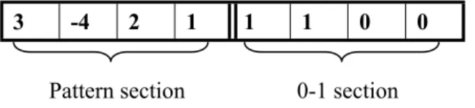
Before coding the cutting patterns, each item is tagged with a natural number like 1, 2, and so on. Consider the example depicted in Figure 1. The chromosome structure has two sections. The first section, namely "pattern section", determines sequence and rotation of items. A minus tag in this section indicates a rotation of 90 degrees for the related item, like item 4 in Figure 1. Because all tags are filled in this section, the length of this section is equal to the number of items.
Second section of the chromosome, namely "0-1 section", includes a sequence of digits, zero and one. Current items will be accommodated in a row, if the value of current locus in the second half is equal to zero. Similarly, current items are accommodated in a column if the current value of second half is one.
0 0 1 1 1 2 -4 3
0-1 section Pattern section
Figure 1 Chromosome structure
In a summary description, items are accommodated regarding their sequence in the first half of chromosome until the existing row or column does not allow any more items; because the width/height in existing row/column is less than width/height of the item which is trying to be placed. Then a new row or column is defined regard to the value of next locus in 0-1 half. This procedure is continued until all items are accommodated in the bin(s); or when no more row or column can be defined in the remained area to accommodate the current item. In this situation, if there is at least one urgent item in non-accommodated items, a new bin will be used; otherwise, the procedure is terminated and the remaining items will be postponed to next production program(s).
Figure 2 shows the pseudo-code of decoding procedure. This algorithm returns O (number of
required bins) and 0-1 Yi variables. Yi=1 indicates that the ith item is accommodated in bin(s);
otherwise it will be postponed to next production program(s).
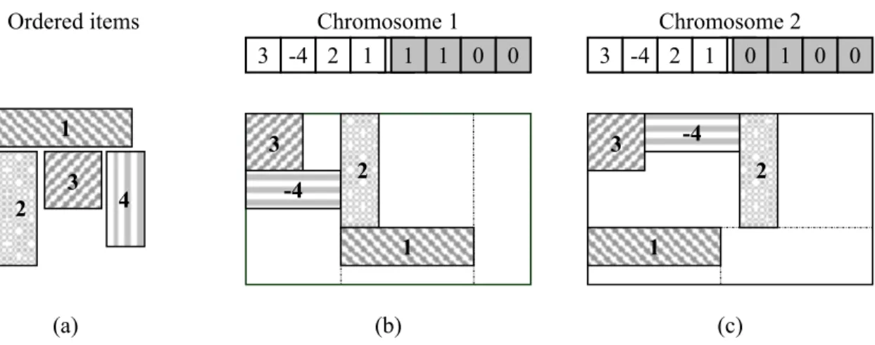
Let us consider two examples to describe decoding procedure. Figure 3(a) shows four ordered items. Figures 3(b) and 3(c) shows two chromosomes and their corresponding decoded patterns generated for these items. These two chromosomes differ in the second half.
In Figure 3(b), because the first allele in second half is equal to one, items are accommodated in a column in the first step. So, item 3 is accommodated in the column at the top left corner. Afterward, item 4 is rotated by 90°, item -4, and then accommodated below the last accommodated item. Subsequently, item 2 should be accommodated. Because item 2 can not be put below the item 4, a new row or column should be considered. As the second allele in second half of the chromosome is again equal to 1, another column is considered in the right side of the previous column and the remaining item(s) is (are) going to be accommodated in the new column. In this simple example all items are accommodated in these two columns and only one bin is required.
In Figure 3(c), because the first allele in second half is equal to zero, items are accommodated in a row in the first step. So, items 3, -4, and 2 are accommodated in this row but item 1 can not be accommodated. Therefore, a new or column is needed and because the second allele in second half is equal to 1, a column is considered below the previous row and remained item(s) is (are) going to be accommodated in this column.
As shown in Figures 3(b) and 3(c), width of a column is determined by the widest item accommodated in the column. Similarly, height of a row is determined by the highest item accommodated in the row. The column width and row height are shown by dashed lines in Figures 3(b) and 3(c).
2.2. Fitness function
Wäscher et al (2007) introduced two basic objective functions: output maximization and input minimization. In the case of output maximization, a set of small items has to be assigned to a given set of large objects (bins). The set of large objects is not sufficient to accommodate all the small items. All large objects are to be used such that a selection (a subset) of the small items of maximal
value has to be assigned. In the case of input minimization, again a given set of small items is to be assigned to a set of large objects. But unlike before, the set of large objects is sufficient to accommodate all small items. All small items are to be assigned to a selection (a subset) of the large object(s) of minimal ‘‘value’’. So, there is no selection problem regarding the small items.
Figure 2 Decoding algorithm
Figure 3 Second half determines the decision of row/column definition
They mentioned that, in some real situations, selection problem exists with respect to both large objects and small items. This requires an extended objective function which combines revenues and costs: profit maximization. Also, there are situations where more than one objective function may have to be taken into account.
The fitness function considered here is multi-objective profit maximization which considers both revenues and costs, based on required bins and waste area. Before describing the fitness function, the following notations are defined:
n total number of items
1
2 3
4
Ordered items Chromosome 1 Chromosome 2
3 -4 2 1 1 1 0 0 3 -4 2 1 0 1 0 0
3
-4 2
1
3 -4
2
1
(a) (b) (c)
SetȜ (Number of required bins) =1;
If the current value in 0-1 section=0, define a row; otherwise, define a column; While all items are not accommodated,
If it is possible, accommodate the current item in the current row/column; SetYi= 1;
Otherwise,
If the next value in 0-1 section=0, define a row; otherwise, define a column;
If still it is not possible to accommodate the current item and there is at least one non-accommodated urgent item,
Set Ȝ = Ȝ + 1; (Use another bin)
Otherwise (there is not any non-accommodated urgent item), Terminate;
Pi value of ith item
yi zero-one variable which indicates the priority of the ith item
Yi zero-one variable which indicates accommodating/ non-accommodating ith item
pr waste value per a unit of weight
wr bin weight per a unit of area
O number of required bins
W bin width
H bin height
wi width of ith item
hi height of ith item
C cost (value) of a bin
The profit of a given chromosome depends on its corresponding pattern. The fitness of a chromosome is equal to its profit.
Profit = Total revenue – Total cost
Total revenue is derived from the value of accommodated items in addition to the value of total waste. Hence,
Profit = PY pr wr
O
WH Y wh CO
n i
i i i n
i i
i »
¼ º «
¬ ª
u
u
¦
¦
1 1
) ( )
(
2.3. Reproduction
At every generation, the two parents are selected with respect to a simple ranking mechanism introduced by Sevaux and Dauzère-Pérès (2003). The population is sorted in descending order with fitness values (descending order with the objective function), so the best individual is ranked first.
The selection of the first parent is made using the probability distribution
2
(
m
1
k
)
/
(
m
(
m
1
))
wherek is the index number of kth chromosome in the descending order of fitness values, and m is
the size of the population. Using this technique, the median chromosome
(
m
1
)
/
2
has theprobability 1/m of being selected, while the best individual has the probability
2
/(
m
1
)
(roughlytwice the median). The second parent is randomly selected with respect to a discrete uniform distribution. Then crossover operators are applied to the two parents and two new offspring are generated.
2.4. Crossover operators
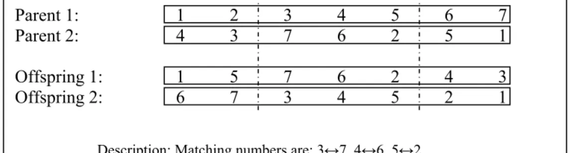
We propose a different type of crossover operator for each section of a chromosome. A PMX (partial matching crossover) crossover operator for the pattern section and a two-point crossover for
the 0-1 section are proposed. Two-point crossover selects two random points in the 0-1 section of the parents` chromosomes and exchanges bits between those two points. In PMX, two crossover points are randomly chosen. Then a matching between the two parents will be done. Figure 4 shows two parents and two offspring generated by PMX operator. Two selected points lead us to
matching: 3ļ7, 4ļ6, 5ļ2.
Only one of the crossover operators will be applied on a chromosome. The applied operator is selected at random; via to generating a random number between 0 and 1 and making it rounded. This way, 0 denotes a PMX crossover so two crossover points are randomly selected in pattern section; while 1 denotes a two-point crossover and two crossover points are randomly selected in 0-1 section. Crossover points are selected regard to a discrete uniform distribution along the genes of the section which is going to be under crossover operation.
Figure 4 Example for result of PMX crossover operator
2.5. Mutation operators
Like crossover operators, two types of mutation operators are implemented for the two sections of the chromosomes. A rotating operator is used for the pattern section which symmetries the value of selected gene. Swap operator is used for 0-1 section which switches between 0 and 1 value. In order to determine which mutation operator to be done, a random locus is selected from the entire length of chromosome based on a discrete uniform distribution. The proper mutation operator is selected regarding the section that the selected locus lies in.
2.6. GA parameters
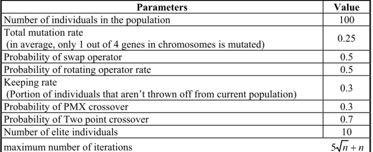
The performance of a GA is generally sensitive to the settings of the parameters that influence the search behavior of the algorithm. The performance of our genetic algorithm depends on some parameters which are explained in this section. In order to set the GA parameters, we consider twenty scenarios and twenty test problems solved under different parameter settings. Each parameter setting has a set of values for GA parameters, like population size, mutation rate, keeping rate, number of elite individuals, etc. The best parameter setting, which resulted in the best results, is used to set the GA parameters. In order to reduce error of random numbers in GA, each problem is solved ten times and average results are reported. Kolmogorov-Smirnov test is implemented for checking the assumption of normality and sufficiency of number of test problems. Afterward, randomized complete block design is used to recognize difference between parameters settings. Finally, Duncan’s multiple-range test is used to choose the best scenario. Consequently, parameters are set as Table 1.
Parent
1: 1 2 3 4 5
6 7
Parent
2: 4 3 7 6 2 5 1
Offspring
1:
1 5 7 6 2 4 3
Offspring
2:
6 7 3 4 5 2 1
Table 1 Parameter values of GA
Parameters Value
Number of individuals in the population 100
Total mutation rate
(in average, only 1 out of 4 genes in chromosomes is mutated) 0.25
Probability of swap operator 0.5
Probability of rotating operator rate 0.5
Keeping rate
(Portion of individuals that aren’t thrown off from current population) 0.3
Probability of PMX crossover 0.3
Probability of Two point crossover 0.7
Number of elite individuals 10
maximum number of iterations 5 nn
3. ADAPTED UPPER BOUND
As mentioned before, the problem variant presented in this paper is not discussed in previous published works. The simplest bound for 2BP problem is the Continuous Lower Bound (CLB) used by different authors, like (Martello and Vigo, 1998). This bound is given by the total area of all elements divided by a bin area:
¸ ¸ ¸ ¸ ¹ · ¨ ¨ ¨ ¨ © § u u
¦
H W h w Ceiling CLB n i i i 1Where, ceiling function rounds its input up, to the nearest integer.
Therefore, we adapted a continuous lower bound found in literature into an upper bound for total profit with considering priority of items. This upper bound is used in analyzing the performance of our proposed approach.
We adapted CLB to consider the priority of items too. For this purpose, we divided ordered items to
two categories: urgent items I1, I2, ..., Im, and postponable items Im+1, Im+2, ..., In. It is clear that all
urgent items, I1 to Im, should be accommodated. In addition, a selection of postponable items can be
accommodated too. Let S denote the set of selected postponable items. Adapted CLB (ACLB) and
profit upper bound (PUB) can be calculated as:
ACLB
¸
¸
¸
¸
¹
·
¨
¨
¨
¨
©
§
u
u
u
¦
¦
H
W
h
w
h
w
Ceiling
i S i i m i i i 1PUB = Total price of all accommodated items + Total benefit of selling waste area
PUB = P P pr wr ACLB
WH w h wh C ACLBS i
i i i
m i
i S
i i m
i
i » u
¼ º «
¬ ª
u u
¦
¦
¦
¦
1
1
Because different permutations of postponable items can be put in the set S, we used an enumerative method which evaluates all permutations of postponable items and reports the best (highest) PUB. We used this best PUB, so called BPUB, in order to analyze the efficiency of the proposed approach.
The run time for this procedure highly increases by the increase of postponable items. With the assumption that the rate of postponable items is little, the run time will be acceptable. For example, in the test problems presented in section 4, at most 10% of items are postponable.
4. COMPUTATIONAL EXPERIMENTS
We adapted ten classes of randomly generated problems presented by the other researchers by adding priority to items and also defining item price, bin value, and so on. The first six classes have been proposed by (Berkey and Wang, 1987):
Class 1: wj and hj uniformly random in (1, 10), W = H = 10;
Class 2: wj and hj uniformly random in (1, 10), W = H = 30;
Class 3: wj and hj uniformly random in (1, 35), W = H = 40;
Class 4: wj and hj uniformly random in (1, 35), W = H = 100;
Class 5: wj and hj uniformly random in (1, 100), W = H = 100;
Class 6: wj and hj uniformly random in (1, 100), W = H = 300;
In each of the above classes, all the item sizes are generated from the same interval.
Martello and Vigo (1998) have proposed four other classes, where a more realistic situation is considered. First, the items are classified into four types:
Type 1: wj uniformly random in (
3
2W, W), hj uniformly random in (1,
2 1H);
Type 2: wj uniformly random in (1,
2 1W),h
j uniformly random in (
3
2H, H);
Type 3: wj uniformly random in (
2
1W, W), hj uniformly random in (
2
1H, H);
Type 4: wj uniformly random in (1,
2 1W),h
j uniformly random in (1,
2 1H);
The Bin sizes are W=H=100 for all classes. We have:
Class 8: type 2 with probability 70%, type 1, 3, 4 with probability 10% each. Class 9: type 3 with probability 70%, type 1, 2, 4 with probability 10% each. Class 10: type 4 with probability 70%, type 1, 2, 3 with probability 10% each.
In each class, we generate five instances with number of items: 20, 40, 60, 80, and 100. We use a 0-1 random variable to define priorities and up to 0-10% of items in each instance are allowed to be postponable. Other parameters are set to comply with real world values. For these problems, prices
and values are derived from the printing industry in Iran. The price of items (pi) is made regard to
the uniform distribution
U
(
0
.
8
w
ih
i,
1
.
2
w
ih
i)
; while multipliers 0.8 and 1.2 denote a 20%tolerance for possible discount or expensiveness. The value of bin (C) is set to
0.3uWH. Thevalue of waste area (pr) is assumed to be 0.2 per one area unit, and bin weight (wr) is 0.1 per one
area unit.
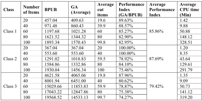
The computer code for this algorithm was written in Matlab 7.0 and was carried out on an AMD Athlon 1.77 with 256 MB of memory. Table 2 shows the results of the computational experiments for 50 solved instances. The first two columns give the class number and the number of items respectively. The next column refers to the best profit upper bound for each instance. For each instance, the performance index (GA solution) / (Best profit upper bound) is reported in percentage. Also average performance index is calculated over the five problems in each class. It is important to mention that the execution time is reasonable for all test problems, not exceeding 3 minutes even for large problems.
The proposed approach has raised acceptable results such that average performance Index is greater than 76% in all classes and in the worst case is 71.59%. Mostly, the gap between GA's best fitness and the best profit upper bound is increased by increasing the number of items. This is because of the roughness of continuous lower bound which becomes significantly unattainable in large problems.
Table 2 Computational results
Class Number
of Items BPUB
GA (Average)
Average cut items
Performance Index (GA/BPUB)
Average Performance Index
Average CPU time (Min)
20 457.04 409.63 19.6 89.63% 1.42
40 971.48 860.43 39.9 88.57% 9.88
60 1197.68 1021.28 60 85.27% 50.88
80 1621.52 1344.32 80 82.90% 148.12
Class 1
100 1893.34 1570.43 99.8 82.95%
85.86%
328.51
20 367.04 367.04 20 100.00% 1.20
40 553.60 553.60 40 100.00% 8.35
60 1291.02 1018.83 59.5 78.92% 43.64
80 1584.86 1332.86 80 84.10% 129.61
Class 2
100 1930.04 1456.34 100 75.46%
87.69%
291.79 20 4621.58 4065.06 19.8 87.96% 1.35
40 8001.94 6451.00 40 80.62% 9.09
60 15029.66 11853.83 59.9 78.87% 50.73 80 17043.22 12847.86 80 75.38% 141.12 Class 3
100 19568.52 14533.13 99.7 74.27%
79.42%
Class Number
of Items BPUB
GA (Average) Average cut items Performance Index (GA/BPUB) Average Performance Index Average CPU time (Min)
20 4082.58 4082.58 20 100.00% 1.21 40 5988.58 5988.58 40 100.00% 8.08 60 12121.60 9321.60 60 76.90% 48.87 80 15776.84 12976.84 80 82.25% 130.79 Class 4
100 20344.10 14744.10 100 72.47%
86.33%
293.49 20 36751.80 31184.51 19.9 84.85% 1.44 40 70926.36 60006.36 40 84.60% 9.66 60 101972.00 83212.00 60 81.60% 50.50 80 139974.20 111351.16 79.9 79.55% 149.14 Class 5
100 185097.10 147695.52 100 79.79%
82.08%
334.39 20 26578.80 26578.80 20 100.00% 1.20 40 74606.80 74606.80 40 100.00% 8.29 60 88711.60 63511.60 60 71.59% 44.81 80 148532.10 123332.08 80 83.03% 130.87 Class 6
100 179740.70 129340.66 100 71.96%
85.32%
297.63 20 30552.74 27752.74 20 90.84% 1.37 40 57715.74 46515.74 40 80.59% 9.30 60 88722.98 69448.39 59.9 78.28% 52.49 80 131964.90 102284.92 80 77.51% 143.80 Class 7
100 169457.30 131937.30 100 77.86%
81.01%
330.13 20 32739.74 27202.19 19.9 83.09% 1.38 40 73543.22 62356.91 39.9 84.79% 9.54 60 83585.96 66414.30 60 79.46% 50.45 80 120210.00 95290.00 80 79.27% 144.85 Class 8
100 158269.00 120749.02 100 76.29%
80.58%
328.19 20 75130.36 55530.36 20 73.91% 1.60 40 101052.50 82716.65 39.9 81.86% 10.44 60 174589.20 129789.24 60 74.34% 53.29 80 253631.60 190491.76 80 75.11% 155.61 Class 9
100 323388.60 248908.60 100 76.97%
76.44%
356.17 20 27717.34 24917.34 20 89.90% 1.33 40 39988.14 32476.00 40 81.21% 9.30 60 57604.88 45284.88 60 78.61% 46.22 80 87668.92 68348.92 80 77.96% 133.55 Class
10
100 101925.80 76725.80 100 75.28%
80.59%
315.71 5. CONCLUTION REMARKS
An extension of two-dimensional bin packing problem is discussed in this paper, where items can have different priorities. The fitness function is to maximize the total profit by considering both revenues and costs, based on required bins and waste area. A genetic algorithm is developed to solve this generalized problem. A new coding scheme is used to code/decode the arrangement patterns. Also an upper bound is presented for the considered problem.
Adapting other lower/upper bounds in the literature to handle priority of items and study of implementing our GA on other packing problem types are interesting fields for future researches.
REFERENCES
[1] Berkey J.O., Wang P.Y. (1987), Two-dimensional finite bin packing algorithms; Journal of the Operational Research Society 38; 423-429.
[2] Correa J.R. (2004), Near-optimal solutions to two-dimensional bin packing with 90° rotations; Electronic Notes in Discrete Mathematics 18; 89–95.
[3] Correa J.R. (2006), Resource augmentation in two-dimensional packing with orthogonal rotations; Operations Research Letters 34; 85–93.
[4] Davis L. (1985), Applying adaptive search algorithms to epistatic domains; Proceedings of the 9th Int. Joint Conference on Artificial Intelligence; 162-164.
[5] Dyckhoff H. (1990), A typology of cutting and packing problems; European Journal of Operational Research 44; 145–159.
[6] Fritsch A., Vornberger O. (1995), Cutting Stock by Iterated Matching; Operations Research Proceedings, Selected Papers of the Int. Conf. on OR 94, U. Derigs, A. Bachem, A. Drexl (eds); Springer Verlag; 92-97.
[7] Hopper E., Turton B. (1997), Application of Genetic Algorithms to Packing Problems: A Review; Proceedings of the 2nd On-line World Conference on Soft Computing in Engineering Design and Manufacturing; Springer Verlag, London; 279-288.
[8] Kröger B. (1995), Guillotineable bin packing: A genetic approach; European Journal of Operational Research 84; 645–661.
[9] Lodi A., Martello S., Vigo D. (1998), Neighborhood search algorithm for the guillotine non-oriented two-dimensional bin packing problem; In S. Voss, S. Martello, L.H Osman, and C. Roucairol, editors, Meta-Heuristics: Advances and Trends in Local search Paradigms for optimization; Kluwer Academic Publishers, Boston; 125-139.
[10] Lodi A., Martello S., Vigo D. (1999), Heuristic and metaheuristic approaches for a class of two Dimensional Bin Packing Problems; INFORMS J. Comput 11; 345–357.
[11] Lodi A., Martello S., Vigo D. (2002), Recent advances on two-dimensional bin packing problems; Discrete Applied Mathematics 123; 379-396.
[12] Lodi A., Martello S., Vigo D. (2004), TSpack: A Unified Tabu Search Code for Multi-Dimensional Bin Packing Problems; Annals of Operations Research 131; 203-213.
[13] Martello S., Vigo D. (1998), Exact solution of the two-dimensional finite bin packing problem; Management Science 44; 388-399.
[14] Polyakovsky S., M’Hallah R. (2009), An agent-based approach to the two-dimensional guillotine bin packing problem; European Journal of Operational Research 192; 767–781.
[15] Puchinger J., Raidl G.R. (2006), Models and algorithms for three-stage two-dimensional bin packing; European Journal of Operational Research 183; 1304-1327.
[16] Sevaux M., Dauzère-Pérès S. (2003), Genetic algorithms to minimize the weighted number of late jobs on a single machine; European Journal of Operational Research 151; 296–306.
[17] Smith D. (1985), Bin-packing with adaptive search; in Grefenstette (ed.). Proceedings of International Conference on Genetic Algorithms and their Applications; Lawrence Erlbaum; 202-206.
[18] Vasko F.J., Wolf F.E., Stott K.L. (1989), A practical solution to a fuzzy two dimensional cutting stock problem; Fuzzy Sets and Systems 29; 259-275.
[19] Wäscher G., Haußn er H., Schumann H. (2007), An improved typology of cutting and packing problems; European Journal of Operational Research 183(3); 1109-1130.