132
A multi-objective genetic algorithm (MOGA) for hybrid flow shop
scheduling problem with assembly operation
Seyed Mohammad Hassan Hosseini1*
1
Department of Industrial Engineering and management, Shahrood University of technology, Shahrood, Iran
Abstract
Scheduling for a two-stage production system is one of the most common problems in production management. In this production system, a number of products is produced and each product is assembledfrom a set of parts. The parts are produced in the first stage that is a fabrication stage and thenthey are assembled in the second stage that usually is an assembly stage. In this article the first stage assumed as a hybrid flow shopwith identical parallel machines and the second stage will be an assemble work station. Twoobjective functionsare considered that are minimizing the makespan, and minimizing the sum of earliness andtardiness of products.At first the problem is defined and its mathematical model is presented. Since the considered problem is NP-hard,themulti-objective genetic algorithm (MOGA) is used to solve this problem in two phases. In the first phase the sequence of the products assembly is determined and in the second phase the parts of each products is scheduled to be fabricated. In each iteration of the proposed algorithm, the new population is selected based on non-dominance rule and fitness value. To validate the performance of the proposed algorithm, in terms of solution quality and diversity level, various test problems are designed and the reliability of the proposed algorithm is compared with two prominent multi-objective genetic algorithms, i.e. WBGA, and NSGA-II. The computational results show that the performance of the proposed algorithms is good in both efficiency and effectiveness criteria. In small-sized problems, the number of non-dominance solution come out from the two algorithms N-WBGA (the proposed algorithm) and NSGA-II are approximately equal. Also more than 90% solution of algorithms N-WBGA and NSGA-II are identical to the Pareto-optimal result. Also in medium problems, two algorithms N-WBGA and NSGA-II have approximately an equal performance and both of them are better than WBGA. But in large-sized problems, N-WBGA presents the best results in all indicators.
Keywords: Multi-objective Genetic algorithm, Two-stage production system, Assembly
*Corresponding author
ISSN: 1735-8272, Copyright c 2017 JISE. All rights reserved
Journal of Industrial and Systems Engineering
Vol. 10, special issue on production and inventory, pp 132-154 Winter (February) 2017
133
1- Introduction
Two-stage assembly scheduling problem contains a machining operation that fabricates and prepares the parts (preassembly stage), and an assembly stage that joins the parts into the products. This production system has applications in many industries, and therefore has received increasing attention from many researchers (Sup Sung, &Juhn, 2009; Lin, &Liao, 2012; Allahverdi, A., &Aydilek, H., 2015; Jung, Woo, & Kim, 2017). For example Lee et al. (1993) described an application in a fire engine assembly plant while Potts et al. (1995) described an application in personal computer manufacturing. In particular, manufacturing of almost all items may be modeled as a two-stage assembly scheduling problem including machining operations and assembly operations (Allahverdi et al., 2009). Despite the importance of this problem, the review studied shows that scant attention has been given to solve it, especially in the case of multiple criteria.
In this paper this problem is studiesd in which that the machining operation is done in a hybrid flow shop and there a work station for the assembly operation. Two objectives are considered for this problem: to minimizemakespan, and minimizing the sum of earliness and tardiness of products.
Most of researches in production scheduling are concerned with the minimization of a single criterion. Up to the 1980s, scheduling research was mainly concentrated on optimizing single performance measures such as makespan (C ), total flowtime (F), maximum tardiness (T ), total tardiness ( ) and number of tardy jobs (n )(Arroyo, &Armetano, 2005). C andF are related to maximizing system utilization and minimizing work-in-process inventories, respectively, while the remaining measures are related to job due dates. However, scheduling problems often involve more than one aspect and therefore require multiple criteria analysis.In allcompanies, each particular department decision makerwants to minimize a special criterion. For examplein a company, the commercial manager is interestedin satisfying customers and then minimizingthe tardiness. On the other hand, the productionmanager wishes to optimize the use of the machinesby minimizing the makespan or the work in processby minimizing the maximum flow time. Each of these objectives is valid from a generalpoint of view. Since these objectives are conflicting,a solution may perform well for one objective,but giving bad results for the others. For this reason,scheduling problems have often a multi-objectivenature (Loukilet al. 2005; Fattahi et al. 2014).
The first study in assembly-type flow-shop scheduling problem was done in 1993 (Lee et al. 1993). A two-stage assembly flow-shop scheduling problem considering a single objective function ( ) was studied by them. They showed that the problem is strongly NP-complete and identified several special cases of the problem that can be solved in polynomial time and suggested a branch and bound solution and also three heuristics. After that Potts et al. (1995) studied and extend the problem with the same objective function as Lee et al. Hariri and Potts (1997) also studied the same problem as Potts et al. with the same objective function and proposed a branch and bound algorithm. Cheng and Wang (1999) considered minimizing the makespan in a two-machine flow-shop scheduling with a special structure and developed several properties of an optimal solution and obtained optimal schedules for some special cases.
In most studies of assembly type scheduling problem, it is assumed that the preassembly stage has a parallel machine format followed by an assembly stage. This production system is named two-stage assembly flow shop. The objective function of these studies is single criterion such as the completion time of all jobs. For example see Koulamas and Kyparisis (2007), Sung and Kim (2008), and Allahverdi and Al-Anzi (2009). In all of these studies it has been shown that the problem is NP-Hard, and hence most of them have presented some approximately solution based on metaheuristic algorithms.
Some studies have been done by Yokoyama (2001, 2008) and Yokoyama et al. (2005) in the assembly type production system in which that the reassembly stage is a two or three stage flowshop. The objective function is still single criterion such asmakespan, mean completion time for all products, and weighted sum of completion time ofeach product. This problem is NP-Hard and they presented some heuristic solutions or B&B algorithm for the special cases of the problem.
Fattahi et al. (2012) introduced the hybrid flow shop with assembly operations for the first time in 2012 . Their objective function is makespan and they considered the preassembly stage as a two-stage hybrid flow shop and presented a mathematical model for the considered problem. Since the considered problem is strongly NP-Hard, they presented some heuristic solution that can solve the problem up to 150 products
134
and 16 parts for each product. A new hybrid improvement algorithm for the finite capacity material requirement planning (FCMRP) system in a flexible flow shop with assembly operations was proposed by Watcharapanand Teeradej (2016). The proposed algorithm is a hybrid of genetic algorithm (GA) and tabu search (TS). There are six primary steps in the proposed algorithm. In step 1, a production schedule is generated by variable lead-time MRP. In step 2, dispatching and random rules are applied to generate initial sequences of orders. From step 3 to step 5, the sequences of orders are iteratively improved by characteristics of TS and GA. Finally, in step 6, the start times of operations are optimally determined by linear programming. The results validate the performance of the proposed algorithm.Allahverdi et al. (2016) also studied the two-stage assembly flowshop scheduling problemwith separate setup times. Their objective considered wasto minimize total tardiness. Some new algorithms have been developed based on different versions of simulated annealing, genetic, andinsertion algorithms by them.
The majority of papers on these problems have concentrated on single-objective problems, while consideration of multiple objectives is more realistic. One of the most differences between this paper and the other similar research is the objective function and solving techniques.
Since multi-objective scheduling problem (MOSP) plays a key role in practical scheduling, there has been an increasing interest in MOSP according to the literature. Hence, there has been a noticeable increase in published the MOSP especiallymulti-objective evolutionary algorithms (MOEA).
Konak et al. (2006) and Sun et al. (2010) presented a review and prospects of multi-objective optimization algorithms. Also Coello et al (2007) presented a comprehensive evolutionary algorithm for solving multi-objective problems. According these studies, being a population-based approach, genetic algorithms (GA) are well suited to solve multi-objective optimization problems. Therefore, GA has been the most popular heuristic approach to multi-objective design and optimization problems.
The first multi-objective GA, called vector evaluated GA(or VEGA), was proposed by Schaffer (1985). Afterwards,several multi-objective evolutionary algorithms were developedincluding Multi-objective Genetic Algorithm(MOGA), Niched Pareto Genetic Algorithm (NPGA), Weight-based Genetic Algorithm (WBGA), RandomWeighted Genetic Algorithm (RWGA), NondominatedSorting Genetic Algorithm (NSGA), StrengthPareto Evolutionary Algorithm (SPEA), improvedSPEA (SPEA2), Pareto-Archived Evolution Strategy (PAES), Pareto Envelope-based Selection Algorithm(PESA), Region-based Selection in Evolutionary Multiobjective Optimization (PESA-II), Fast NondominatedSorting Genetic Algorithm (NSGA-II),Multi-objective Evolutionary Algorithm (MEA),Micro-GA, Rank-Density Based Genetic Algorithm(RDGA), and Dynamic Multi-objective EvolutionaryAlgorithm (DMOEA) (Coello et al. 2007 and Konak et al. 2006).
To illustrate the novelties of this paper, the following items could be presented:
• To properly address the hybrid flow shop scheduling problem with assembly operation in multi-objective condition. The goals of JIT production management is added as a new multi-objective.
• To develop a mathematical programing model for the considered problem.
• A new extension of MOGA with a new approach in two phases to solve the considered problem in large-sized scale.
• Using both the non-dominated solutions and weighted average of the normalized objectives in the generation transmissionof the proposed algorithm.
This paper proceeds as follows: In section 2, the problem is described completely. The multi-objective optimization and some common techniqueswill be expressed in section 3. The proposed solving algorithm is presented in section 4. In section 5, designing of the problems and Computational experiment and results is presented. Finally, a Concluding remarks and summary of the work and direction for the future research are given in section 6.
135
2- Problem description
The scheduling problem for a two-stage production system with multi-objective criteria is considered in this paper. This system contains a hybrid flow shop stage followed by an assembly stage. Suppose that several products of different kinds ( )are ordered andeach product needs a set of parts ( = 1, 2, 3, … , ) to complete. At first, the parts are manufactured in a two-stage hybrid flow shop. Each part
has a fixed processing time on stage . The machines are identical in the hybrid flow shop and the number of machines is K , K! on stage one and two of the hybrid flow shop respectively. After manufacturing the parts, they are assembled into the products on an assembly stage. The assembly operationscannot be started for a product until the set of parts is completed in machining operations. The considered objective is to minimize makespan and the sum of earliness and tardiness (C , ∑ E$ $/T$). Decision variables are sequence of the products to be assembled and also sequence of the parts and assigning them to machines in each stage of the hybrid flow shop to be processed.
One of the applications of this problem is body making of car manufacturing industry. A car making manufactory generally contains the units of production engine, chassis and body. The unit of body making includes a press shop, assembly and painting. The press shop that produces some parts such as doors and roofs has usually a flow shop or hybrid flow shop format.
Usually in these systems the inputs contain raw material, parts or unfinished products that are processed in a hybrid flow shop. When the set of parts of a product complete, they are joined on assembly stage. Typically, buffers are located between stages to store intermediate products and it is supposed that there is no limited in buffer storages. The number of machines in hybrid flow shop stages is free and it can be no equivalent at two stages.
2-1- Notations
The notation of the proposed problem can be introduced as bellow: H Total number of products
h Product index (h = 1, 2, . . . , H) n Total number of parts
j Part index (j = 1, 2, . . . ,n)
Total number of parts of product h (h = 1, 2, . . .,H) l Stage index (l=1,2)
Processing time of machining operations for part j in stage l (l=1, 2) & Number of parallel machines in stage l
k Machine index,
' Assembly time of product h ( Due date for delivery of product h M A very big and positive amount
Also variables of the mathematical model are as follow:
)* + 1, if job j is processed directly after job i on machine k in stage l, 0 otherwise, ),*+ 1, if job i is the first job on machine k in stage l, 0 otherwise,
)*,+ 1, if job i is the last job on machine k in stage l, 0 otherwise, - ) Completion time of job j in stage l,
. Finish time of the parts for hth product and ready to assemble
/ ′ 0, if all parts of product ℎ′ is ready to assemble before the parts of product h, a positive amount otherwise,
Completion time of assemble of the product h 1 Earliness of completion time of the product h
Tardiness of completion time of the product h
136
The problem is to decide about sequencing of the products and their parts, and the objective function of the considered problem is expressed as:
Min 5 = 678)- ) , ∑ -1 / )34 9 or : , 2;
While 2 is a function of earliness and tardiness and computed as (1)
2 = <=>78)-0 , − ( ) + 78)-0 , ( − )B 3
4
C (1)
2-2- Assumptions
(1) All parts are available at time zero.
(2) There are two series satge with some parallel machines in each stage for fabrication the parts.
(3) The parallel machines in each stage are uniform.
(4) If product h is going to be assembled before product h', then, on each stage, processing of any part of product h' doesn't start before starting the processing of all parts for product h.
(5) Assembly operations for a product will not start until all parts of its product are completed.
(6) When assembly operations of a product is start, it doesn't stop until completed (no preemption in assembly stage)
(7) There is no limited in buffer storages 2-3- Numerical example
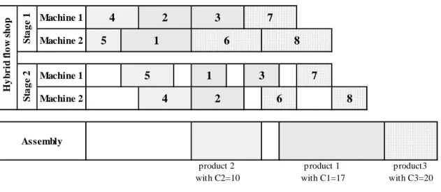
In order to clarify the problem, consider a simple numerical example as table 1. Assume that there are two machines at stage 1 and two machinesat stage 2. Also, there is an assembly stage at the end of the production system. Total number of products is = 3and the data for parts and their processing time of machining operations and assembly are given in table 1.
Table 1. Processing time of machining and assembly
Stage (l)
Products and parts
Product 1 Product 2 Product 3
j=1 j=2 j=3 j=4 j=5 j=6 j=7 j=8
Stage 1 4 3 3 3 2 4 3 4
Stage 2 2 3 2 3 3 2 2 2
Assembly 6 4 3
Due date 16 12 22
One solution for scheduling the products and their parts is shown in figure 1. According this solution, the products will be produced in a sequencing of 2-1-3 and scheduling the parts of each product is according their numbers in both of two stages of the hybrid flow shop. This solution leads in result of C = 20 , D = 5.
137
Fig 1. A solution of the example with C = 20 and D = 5
2-4- Mathematical modeling
The mathematical definition of a multi-objective problem (MOP) is important in providing a foundation of understanding between the interdisciplinary nature of deriving possible solution techniques (deterministic, stochastic); i.e., search algorithms. Fattahi et al. (2012)presented a mathematical model for the assembly flexible flow shop scheduling problem with a single objective. Their model is developed for the considered problem in this study. Thus, there is not one unique solution but a set of solutions. Theses set of solutions is found through the use of Pareto Optimality Theory (Coello et al. 2007).Note that multi-objective problems require a decision maker to make a choice of x∗ values. The selection is essentially a tradeoff of one complete solution x over another in multi-objective space.
Based on the notations, the mathematical formulation of the problem is presented as follows: Machine 1
Machine 2
Machine 1 Machine 2
parts machining and assembly operations for product 1 parts machining and assembly operations for product 2 parts machining and assembly operations for product 3
Assembly H y b r id f lo w s h o p S ta g e 1 S ta g e 2 5 4 5 1 2 4 product3 with C3=20 product 1 with C1=17 product 2 with C2=10 7 8 7 8 1 2 3 6 3 6
Min 5 = (2)
Min 5!= 2 (3)
Subject to: = = )* + HI +4 = 1 J *4,,*K
j=1,2,3,…,n l=1,2 (4)
= )* + J 4,
≤ 1
M = 1 , 2 , … , &
i=0,1,2,3,…,n l=1,2
(5)
=J )* +
*4,,*K − = ) +
J 4,, K
= 0
M = 1 , 2 , … , &
h=1,2,3,…,n l=1,2
138
Equations (2) and (3) determine the objective functions ofthe given problem that are minimizing the maximum completiontime (makespan) and the sum of earliness and tardiness,respectively. Constraints (4), (5) and (6) ensure that each part is processed precisely once at each stage. In particular, constraint (4) guarantees that at each stage l for each part JO there is a unique machine such that either JO is processed first or after another job on that machine. The inequalities (5) imply that at each stage there is a machine on which a part has a successor or is processed last. Finally, at each stage for each part there is one and only one machine satisfying both of the previous two conditions by (6).
Constraints (7) and (8) take care of the completion times of the parts at stage 1, 2. Inequalities (7) ensure that the completion times * and of parts i and j scheduled consecutively on the same machine respect
*- )+ = )* + HI
+4
× + Q= )* + − 1
HI
+4
R × S ≤ - ) i=1,2,3,…,n j=1,2,3,…,n l=1,2 (7)
- )+
! ≤ -!) j=1,2,3,…,n (8)
-!)≤ . ∀ ∈ : ; , h=2,3,4,…,H (9)
. + ' ≤ h =1,2,3,…,H (10)
V+ ' − / V × S ≤ h , h' = 1,2,3,…,H , ℎW ≠ ℎ (11)
/ V = Y 1 Z[ . V ≥ .
0 ]^ℎ_`aZb_c h , h' = 1,2,3,…,H , ℎW ≠ ℎ (12)
C$≤ C h=1,2,3,…,H (13)
1 ≥ -( − ) h=1,2,3,…,H (14)
≥ - − ( ) h=1,2,3,…,H (15)
2 = =>1 + B 3
4
h=1,2,3,…,H (16)
)dOef ∈ :0,1;
i=1,2,3,…,n , j=1,2,3,…,n , l=1,2
k ≤ 1,2, … , Kf
(17)
O-f)≥ 0 j=1,2,3,…,n l=1,2 (18)
E$≥ 0 h=1,2,3,…,H (19)
139
this order. Inequality (8) implies that the parts go through the stages in the right order, i.e. from stage 1 to stage 2. Inequalities (9) take care of the start times of the products at the assembly stage. The inequalities (10), (11), and (12) express the completion time of products. Inequalities (11) and (12) ensure that the completion time of product h and h' scheduled consecutively on the assembly stage respect this order. The constraint that the makespan is not smaller than the completion time of any product is expressed by constraints (13). Calculating the earliness and tardiness is shown in equations (14), and (15), respectively and the equation (16) presents the sum of earliness and tardiness for all products. The last four constraints specify the domains of the decision variables.
3- The Multi-objective Optimization
3-1- The Multi-objective Optimization Problem
The Multi-objective Optimization Problem (MOP) that also called criteria optimization, multi-performance or vector optimization problem, can be defined (in words) as the problem of finding (Coello et al 2007):
A vector of decision variables which satisfies the constraints and optimizes a vector function whose elements represents the objective functions. These functions form a mathematical description of performance criteria which are usually in conflict with each other. Hence, the term “optimizes” means finding such a solution which would give the values of all the objective functions acceptable to the decision maker.
The decision variables are the numerical quantities for which values are to be chosen in an optimization problem. These quantities are denoted as h, = 1, 2, 3, … , .
The vector h of decision variables is represented by: h = -) , )!, )i, … , )J)
Where indicates the number of variables.
Also the vector function f-x) of M objectives is represented by: f-x) = >f -x), f!-x), fi-x), … , fe-x)B
Having several objective functions, the notion of “optimum” changes, because in MOPs, the aim is to find good compromises (or “trade-offs”) rather than a single solution as in global optimization. In this condition the optimum concept is also changed and the most commonly accepted term is Pareto-optimal. In words, h∗ is a solution of thePareto-optimal if there exists no feasible vector h which would decrease some criteria without causing a simultaneous increase in at least one other criterion (assuming minimization). The objective vectors corresponding of the Pareto-optimal solutions are termed non-dominated. A general definition of dominance solution is as follows (Karimi et al. 2010):
A vector k = -l , l!, li, … , l+)is said to dominatem = -n , n!, ni, … , n+) if and only if k is partially less than m, i.e:
∀Z ∈ :1, 2, 3, … , M; , l*≤ n*∧ ∃Z ∈ :1, 2, 3, … , M; , l*< n*.
When a vector is dominated by no other solutions, it is called dominated vector and the non-dominated vectors are collectively known as the Pareto-front. Generally in MOPs, the main goal is to find the Pareto-frontand the decision maker select one of the solution on Pareto-frontbase on more analysis and trade-offs.
The normal procedure to generate the Pareto-frontis to computemany points in solution spaceΩ and their corresponding objective space [-Ω). When there are a sufficient number of these, it is then possible to determine the non-dominated points andto produce the Pareto-front.
140 3-2- The Multi-objective Optimization techniques
There are many approaches that can be used for solving MOPs, that is, to find the Pareto-optimal solutions or at least an approximation to it. These algorithms can be categorized into two major classes of algorithms, the exact and the approximate (heuristics).
Exact algorithms are guaranteed to find an optimal solution and to prove its optimality for every instance of an MOP. The run-time, however, often increases dramatically with the instance size, and often only small or moderately-sized problems can be solved in practice to provable optimality.
Two exact methods are described as below: The linear Combination of Weights
This method combines multiple objectives into an aggregated scalar objective function by multiplying each objective function by a weighting factor and summing up all terms. The new objective function will be as (21):
5 = 7Z ∑ a+*4 *[*-h) (21)
Subject to: h ∈Ω
Where a*≥ 0 for all iand ∑ a* * = 1. By varying these weights we can find all non-dominated points, for problems with a convex non-dominated set.
The r − stuvwxyzuw Method
The { − Constraint is another well known technique used to solve MOPs. In this approach, we optimize one of the objective functions using the other objective functions as constraints. Then by varying constantly the constraint bounds we can obtain all non-dominated points. The { − Constraint problem can be formulated as (22):
5 = 7Z ‚[ -h)ƒ (22)
Subject to:
[*-h) ≤ „*[]`Z = 1, 2, 3, … , M8 (Z ≠
Where εd are assumed values of the objective functions that must not be exceeded. The idea of this method is to minimize one (the most preferred or primary) objective function at a time, considering the other objectives as constraints bound by some allowable levels εd. By varying these levels εd, the non-inferior solutions of the problem can be obtained.
Heuristics are simple procedures that provide good feasible solutions in a reasonable computation time, but not necessarily an optimal one. In harder problems, with many objectives and large instances, the exact algorithms might not be able to solve it or when they do it they take too much time.Hence, many metaheuristic have been implemented to obtaina good solution in acceptable time. Among these techniques, the potential of evolutionary algorithms for solving multi-objective optimization problems was hinted as early as the late 1960s by Rosenberg in his PhD thesis (Coello et al. 2007). After that many researcher implement the evolutionary algorithms especially genetic algorithms (GAs) to solve the NP-Hard problems.
Konak et al. (2006) presented an overview and tutorial of genetic algorithms developed for problems with multiple objectives. The first multi-objective GA, called vector evaluated genetic algorithm (VEGA), was proposed by Schaffer. After that, several multi-objective evolutionary algorithms were developed and implemented.
3-3- Fitness assignment and diversity mechanism
Implementation of GA in multi-objective optimization needs two important considerations: Fitness assignment and diversity mechanism.
141 3-3-1- Fitness assignment
Fitness assignment is used to rank the solutions in order to select the parents, doing the crossover and mutation operations and select the new population in each generation.
The simplest and classical approach to fitness assignment of solutions in MOGA is to assign a weight wd to each normalized objective function fd′-X) so that the problem is converted to a single objective problem with a scalar objective function as follows:
Min Z = w f′
-X) + w!f!′-X) + … + wefe′-X)
Where fd′-X) is the normalized objective function fd-X)and ∑ wd= 1. The main difficulty with this approach is selecting a weight vector for each run.
Another fitness assignment is altering objective functions. In this method the population PŠ is randomly divided into & equal sized sub-populations -P , P!, … , P‹, ). Each solution in subpopulation PdAssigns a fitness value based on the objective functionZd. Solutions are selected from these subpopulations using proportional selection for crossover and mutation.
The third technique is Pareto-ranking approaches that utilize the concept of Pareto-dominance in evaluating fitness or assigning selection probability to solutions. The population is ranked according to a dominance rule, and then each solution is assigned a fitness value based on its rank in the population. The first Pareto-ranking technique was proposed by Goldberg (Ehrgott 2005) and after that several methods have been proposed (see Coello et al. 2007).
3-3-2- Diversity mechanism
Diversity mechanism is need to obtain solutions uniformly distributed over the Pareto-front. Without taking preventive measures, the population tends to form relatively few clusters in multi-objective GA. This phenomenon is called genetic drift, and several approaches have been devised to prevent genetic drift as follows.
The first approach is fitness sharing that encourages the search in unexplored sections of a Pareto-front by artificially reducing the fitness of solutions in densely populated areas. To achieve this goal, densely populated areas are identified and a penalty method is used to penalize the solutions located in such areas. The second approach is crowding distance that aim to obtain a uniform spread of solutions along the best-known Pareto-front without using a fitness sharing parameter.
Finally the third approach is cell-based density. In this approach the objective space is divided into K-dimensional cells. The number of solutions in each cell is defined as the density of the cell, and the density of a solution is equal to the density of the cell in which the solution is located. This density information is used to achieve diversity similar to the fitness sharing approach.
4- The proposed solving algorithm
4-1- General scheme of the proposed algorithm
Multi-objective optimization was originally conceived with finding Pareto-optimal solutions (Pareto, 1981), also called efficient solutions. Such solutions are non-dominated, i.e., no other solution is superior to them when all objectives are taken into account. Since in GA a population-based approach is used, it is well suited to solve multi-objective optimization problems, and hence several multi-objective evolutionary algorithms were developed after presenting the first multi-objective GA by Schaffer (Coello et al. 2007). Therefore a heuristic based on GA is proposed for the considered problem in this paper. The pseudo-code of the proposed algorithm is as algorithm (1):
142
Algorithm 1 The pseudo code of the proposed algorithm
1) Step 0: Initialization (population size, fitness, crossover and mutation operations, and stopping criterion)
2) Step 1: Start with an initial population , and set t = 0. 3) Step 2: If the stopping criterion is satisfied, return PŠ.
4) Step 3: Evaluate the fitness value of the population as weighted sum approach. 5) Step 4:Use a stochastic selection method based on fitness value to select parents. 6) Step 5: Apply crossover and mutation on parents to generate child population Υ
.
7) Step 6: Evaluate fitness value of the Υ as weighted sum approach.
8) Step 7: Set ^ = ^ + 1 and select • from • and Œ•according the nondominance property and the fitness values to create new generation (see section4.6).
9) Step 8: Go to step 3
4-2- Solution representation
Implementation a metaheuristic needs to decide how to represent and relate solutions in an efficient way to the searching space. Representation should be easy to decode and calculate to reduce the run time of algorithm. In the considered problem,several products ( ) of different kinds are ordered to be scheduled and produced. Each product needs a set of parts (J$ = 1, 2, 3, … , n$) to complete that fabricated in a hybrid flow shop.
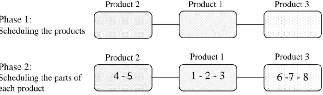
According the assumption (3), If product ℎ is going to be assembled before product ℎ′, then, process operations of all parts of the product ℎ′ doesn't start before processing of all parts of the productℎ. Hence in proposed algorithm the product and the parts are scheduled in two phases separated. During phase 1, the sequence of the products is determined and then, sequencing of the parts is done for each product in phase 2. For example consider the numerical example that illustrated in section 2.3 . Two steps of scheduling of this problem can be done as figure 2.
Fig 2. An example of the two-phases scheduling
In order to coding the solutions as chromosomes in GA proposed algorithm, each solution (sequence)isconsidered in a two-row matrix that the above row shows the number of products and the below indicates the parts of the above product. For example the sequence of the figure 3 is shownas figure 3.
Product number: 2 2 1 1 1 3 3 3
Part number: 4 5 1 2 3 6 7 8
Fig 3.Presentation the products and their parts as a chromosome
Product 1 Product 3
Product 2
Phase 1:
Scheduling the products
Product 2 Product 1 Product 3
Phase 2:
Scheduling the parts of each product
143
The schedule of the parts in each product is considered only on stage 1. After that, each part that release earlier from stage 1, will process on stage 2.
The chromosome and probability of crossover and mutation is defined as below: Chromosome: Each sequence of all products including sequence of their parts.
Ž••: Probability of crossover operation on products in each chromosome.
Ž• : Probability of crossover operation on the parts of each product in every chromosome. ‘••: Probability of mutation operation on products in each chromosome.
‘• : Probability of mutation operation on the parts of each product in every chromosome.
Crossover and mutation operation is implemented on product and their parts in each chromosome separately.
4-3- Initialization
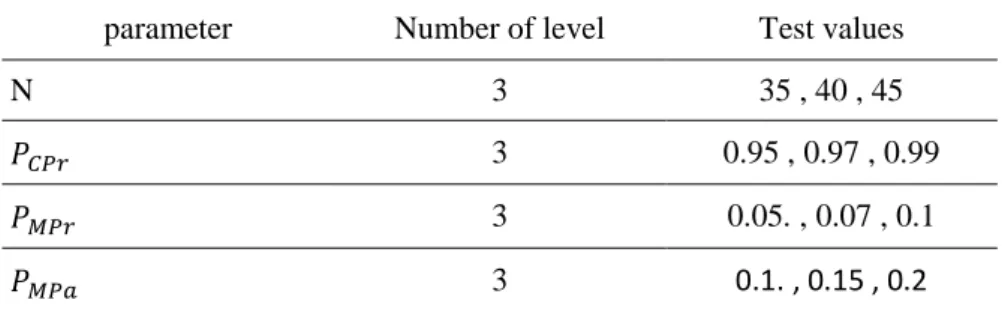
The best value of the parameters for the proposed algorithm is obtained using Taguchi settings considering plan of ’J in three levels. In order to determine the best combination of these parameters, three levels of each parameters was examined as table 2.
Table 2. The values of the parameters of hybrid proposed algorithm parameter Number of level Test values
N 3 35 , 40 , 45
Ž•• 3 0.95 , 0.97 , 0.99
‘•• 3 0.05 , 0.07 , 0.1 .
‘• 3 0.1 , 0.15 , 0.2 .
Due to the considered problem is a two-objective problem, the S“2 index is used to determine better solution as equation (23).
S“2 = ∑–•—˜”•
J
when ™* = š[*!+ [*!! ∀Z = 1. 2. … .
This index is calculated for each set of pareto solution. So, for each 27 cases of Taguchi plan a number will be obtained. Based on this number, comparison the Relative Percentage Deviation (RPD) will be possible.
Finally, after doing experiments, the best combination of the parameters for the proposed algorithm was determined as below:
œ = 40
Ž•• = 0.95
Ž• = 0
‘••= 0.1
‘• = 0.2
Also, in order to reduce the run time of algorithm, it is better to do mutation operator only on the parts. Hence, it supposed that Ž• = 0.
The stopping criterion is the number of iterations and it is considered as a variable that is equal to the number of products in each problem but it must be at least 30 iterations.
The fitness value is calculated as the weighted sum approach. Hence, at first the objective functions have to be normalized. We define [ -)) and [Ÿ-)) as objective function for the makespan and deviation of due (23)
144
date respectively. Therefore the normalized of these two objective functions for each solution is calculated as (24) and (25):
[′ -)) = ¡- )
∑
¡- )
∈•¢
(24)
[Ÿ′-)) = ∑ £- )
£- )
∈•¢
(25)
Finally the fitness value (fv) for each solution (x) is obtained as (26):
[n-)) = a × [′-)) + a!× [
Ÿ′-))
(26) The weight of w and w! is assumed the same and equal to 0.5.
4-4- The initial population ¤¥
Most evolutionary algorithms use a random procedure to generate an initial set of solutions. However, since the output results are strongly responding to the initial set, it is better that some of the initial solutionsare identified as suitable rules.Hence, in initial population three solutions are determined in regulative as below and the others are generatedrandomly.
• One solution is determined based on the earliest due date (EDD) of the product.
• The second solution is determined according non-increasing in assembly time.
• The third is determined according non-decreasing in assembly time.
After generation the initial sequencing for the products, all of the parts are scheduled randomly. 4-5- Selection, recombination and mutation
Selection is done based on the roulette-wheel rule. After calculation the fitness value (fv-x)) for the solutions as equation (25), the operation of the roulette-wheel is done to select the parents.
There exist a variety of crossover operators for recombination that are suitable for the scheduling problems. We tested some of them and finally two operators that were selected for the proposed algorithm are: one-point crossover (1PX), and two-point crossover (2PX).
The mutation operator used here is the insertion operator, which randomly selects a product or a part in the sequence and inserts it in a random position of the sequence.
4-6- Selection the new generation ¤w§¨
The new generation PŠ§ is selected from the current generation and the offspring -PŠ⋃QŠ) based on dominance rule and also considering the fitness values. In other word, first all of the solutionsofthe non-dominated set are selected for the new generation and the remained required solution is selected from the points with the more fitness value to complete the new generationPŠ§ .
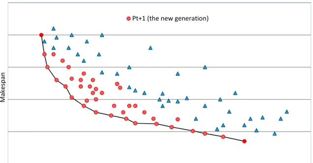
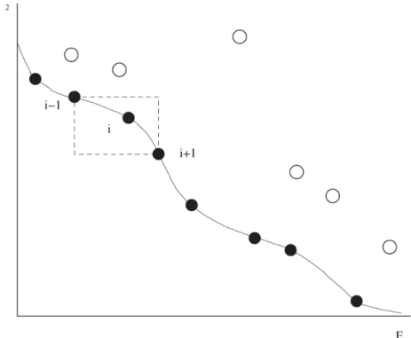
Figures 4 and 5 show an example of this rule in selection a new generation. Figure 4 shows PŠ (the current generation) and QŠ (the offspring). As the above rule, the new generation is selected as it is shown in figure 5.When the solutions of the non-dominated set is more than the population size, only those that are maximally apart from their neighbors according to the crowding distance are chosen.
145
Figure 6 presents a graphical illustration of crowding for an example and the computations are done as (27) to (29).
Fig 4. Forty solutions with maximum of the fitness value between total parents and their offspring
Fig 5. Selection the new generation oftotal parents and their offspring
M
a
k
e
sp
a
n
Sum of earliness and tardiness
Pt (current generation) Qt (the offspring)
M
a
k
e
sp
a
n
Sum of earliness and tardiness Pt+1 (the new generation)
146
Fig 6. A graphical illustration of crowding
(* =[ -)[*§ ) − [ -)*«− [ *J ) (27)
(*! =[!-)*§[ ) − [!-)*« )
! − [! *J (28)
(* = (* + (*! (29)
The proposed algorithm that used both the non-dominated solutions and weighted average of the normalized objectives based on the genetic algorithm is called as N-WBGA in this article.
5- Computational experiments and results
In this section, the computational experimentsare carried out in order to evaluate the performance of the proposed algorithm. The tests have been performed on various condition of the problem. The considered algorithms are coded in MATLAB 7/10/0/499 (R2010a). The experiments are executed on a Pc with a 2.0GHz Intel Core 2 Duo processor and 1GB of RAM memory.
5-1- Design of problems
To show the efficiency of the proposed algorithm, it is necessary to design problems in a variety wide of conditions and test the proposed algorithm by them. Hence, the processing and assembly times have been generated from a discrete uniform distribution with a defined range to provide three conditions: (a) the hybrid flow shop is a bottleneck, (b) the assembly stage is a bottleneck, and (c) there is a balance condition between two stages. In order to evaluate the algorithms, each problem has been run ten times and solved
147
by the algorithms. In each run, the processing and assembly times have been generated in a defined ranges randomly.
Also, in the scheduling problems that the earliness and tardiness are considered in the objective function, the problems are designed in a variety wide of due date. Hence the researchers have considered two significant factors consisting the tardiness (τ) and the range of due date (R) in these problems (Moslehi et al. 2009). Generally, by considering these two factors, the due dates can be obtained as (30):
( = ¬-1 − ® −¯2° × S , -1 − ® +¯2° × S± (30)
Researchers usually design the problems by changing the factors ®and ¯. Moslehi et al.(2009), present that when ® = 0.2and = 0.6 , the primary jobs of the sequence have earliness, and the remaining ones often have tardiness. This combinatorial is considered in this study and so due date of the product is defined within a discrete uniform distribution with a rangeof>0.5S , 1.1SB. Sis the maximum completion times of all jobs that usually is obtained from an exist algorithm and we use the GRASP algorithm to obtain S.
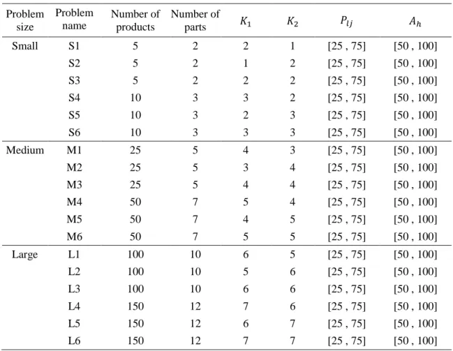
Table 3.The test problems Problem
size
Problem name
Number of products
Number of
parts & &! '
Small S1 5 2 2 1 [25 , 75] [50 , 100]
S2 5 2 1 2 [25 , 75] [50 , 100]
S3 5 2 2 2 [25 , 75] [50 , 100]
S4 10 3 3 2 [25 , 75] [50 , 100]
S5 10 3 2 3 [25 , 75] [50 , 100]
S6 10 3 3 3 [25 , 75] [50 , 100]
Medium M1 25 5 4 3 [25 , 75] [50 , 100]
M2 25 5 3 4 [25 , 75] [50 , 100]
M3 25 5 4 4 [25 , 75] [50 , 100]
M4 50 7 5 4 [25 , 75] [50 , 100]
M5 50 7 4 5 [25 , 75] [50 , 100]
M6 50 7 5 5 [25 , 75] [50 , 100]
Large L1 100 10 6 5 [25 , 75] [50 , 100]
L2 100 10 5 6 [25 , 75] [50 , 100]
L3 100 10 6 6 [25 , 75] [50 , 100]
L4 150 12 7 6 [25 , 75] [50 , 100]
L5 150 12 6 7 [25 , 75] [50 , 100]
L6 150 12 7 7 [25 , 75] [50 , 100]
The testing data is divided into the small problems, the medium problems, and the large problems by changing the parameters. The following parameters are considered to design and generate these problems totally:
Numbers of jobs ( ): 5, 10, 25, 50, 100, and 150.
Number of machines on stages of HFS ( Process time of the parts on stages 1 and 2 ( range of [25, 75].
Assembly times of a product (' 100].
Due date for delivery of product h ( >0.5S , 1.1SB.
By combination of all parameters, the problems and their data are defined as table 5-2- Comparisons of results
This section presents the results of the times by the algorithm. The best and the areevaluated in this section.The performance
problems is evaluated in comparison of the result of the mathematical model and also two techniques WBGA and NSGA-II.
5-2-1-Small-sized problems
At first, the experiment is carried out on the
the small-sized problems and its performance is compared, based on some comparison metrics, with the two other multi-objective genetic algorithms WBGA and NSGA
optimal is needed that is obtained from the mathematical model.
There are a number of methods available to compare the performance of different algorithms. Rahimi Vahedet al.(2007) and many other researchers use the number of Pareto
measure of the performance of the algorithms studied. The
(ONVG), the Overall Non-dominated Vector Generation Ratio (ONVGR), the thegenerational distance (GD) are als
optimal solutions areknown (Coello et al. 2007) explained in the next sections.
5-2-1-1- Number of pareto-optimal solutions
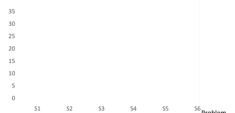
The first result about the performance of the proposed
shows the number of pareto-optimal solution that the proposed algorithm could find in comparision of total number. The total number is obtained by solvin
performance of the proposed algorithm in this index.
Fig 7. Finding pareto
0 5 10 15 20 25 30 35 S1 N u m b e r o f p a re to -o p ti m a l 148
on stages of HFS (&): 1, 2, 3, 4, 5, 6, and 7.
Process time of the parts on stages 1 and 2 ( ): generated from the discrete uniform distribution with
' ): generated from the discrete uniform distribution with delivery of product h (( : generated from the discrete uniform distribution with
of all parameters, the problems and their data are defined as table
This section presents the results of the algorithm described in section 4. Each problem has been run ten best and the average of results obtained of ten runs of each problem The performance of the proposed algorithm
(N-problems is evaluated in comparison of the result of the mathematical model and also two II.
t is carried out on the small-sizedproblems. The proposed algorithm is applied to sized problems and its performance is compared, based on some comparison metrics, with the
objective genetic algorithms WBGA and NSGA-II. In these comparisons the is needed that is obtained from the mathematical model.
There are a number of methods available to compare the performance of different algorithms. Rahimi and many other researchers use the number of Pareto-solutions as a quantitative measure of the performance of the algorithms studied. The Overall Non-dominated Vector Generation
dominated Vector Generation Ratio (ONVGR), the
are also used as the performance measureindicators when the Pareto (Coello et al. 2007). The comparison metrics that we implemented are
optimal solutions
The first result about the performance of the proposed algorithm is presented in figure 7. This figure optimal solution that the proposed algorithm could find in comparision of total number. The total number is obtained by solving the mathematical model. This result shows a good performance of the proposed algorithm in this index.
inding pareto-optimal solutions using the proposed algorithm
S2 S3 S4 S5 S6
): generated from the discrete uniform distribution with a ): generated from the discrete uniform distribution with a range of[50, : generated from the discrete uniform distribution with a range of of all parameters, the problems and their data are defined as table 3.
. Each problem has been run ten average of results obtained of ten runs of each problem -WBGA) in solving the problems is evaluated in comparison of the result of the mathematical model and also two powerful
The proposed algorithm is applied to sized problems and its performance is compared, based on some comparison metrics, with the In these comparisons the Pareto-There are a number of methods available to compare the performance of different algorithms. Rahimi-solutions as a quantitative dominated Vector Generation dominated Vector Generation Ratio (ONVGR), the error ratio (ER), and o used as the performance measureindicators when the
Pareto-The comparison metrics that we implemented are
lgorithm is presented in figure 7. This figure optimal solution that the proposed algorithm could find in comparision of g the mathematical model. This result shows a good
optimal solutions using the proposed algorithm S6
149
5-2-1-2- Overall Non-dominated Vector Generation (ONVG)
The Overall Non-dominated Vector Generation (ONVG) measures the total number of non-dominated vectors found during algorithm execution. This Pareto-non-compliant metric is defined as equation (31).
³´µ¶ = |¤¸¹utºu| (31)
5-2-1-3- Overall Non-dominated Vector Generation Ratio (ONVGR)
Overall Non-dominated Vector Generation Ratio (ONVGR) measures the ratio of the total number of non-dominated vectors found PFe»¼½»during algorithm execution to the number of vectors found in ¾¿ÀÁÂÃ. This metric indicator is calculated as equation (32).
ONVGR =|¾¿ÉÊËÌÊ|
|¾¿ÀÁÂÃ| (32)
When ONVGR = 1, this states only that the same number of points have been found in both ¾¿ÀÁÂÃand ¾¿ÉÊËÌÊ. It does not infer that ¾¿ÀÁÂÃ= ¾¿ÉÊËÌÊ.
5-2-1-4- Error Ratio (ER)
After finishing the solving process, the number of solutions on the finalPareto-front (¾¿ÉÊËÌÊ) is termed as |¾¿ÉÊËÌÊ| and the number of solutions on the optimumPareto-front -¾¿ŠÍÎÏ)is termed as |¾¿ÀÁÂÃ|. The Error Ratio (ER) metric reports the number of solutions on the final Pareto-front -|¾¿ÉÊËÌÊ|)that are not members of the optimum Pareto-front -|¾¿ÀÁÂÃ|) [21]. This metricwhich is Pareto-compliant, requires that ¾¿ŠÍÎÏ is known and that the proposed algorithm approaches the Pareto-front. In this study the lingo is used to obtain the ¾¿ŠÍÎÏ for the small problems according the proposed mathematical modeling and varying the a*. After determining the ¾¿ÉÊËÌÊby proposed algorithm and the PFŠÍÎÏby lingo, ER is calculated as (33).
1¯ =∑| .|•Ð*4Ñ–ÒÓ–|_*
+JÔÕJ|
(33)
Where ed is one if the iŠ$ vector of PFe»¼½»is not an element of PFŠÍÎÏ. When 1¯ = 1, this indicates that none of the points in PFe»¼½» are in PFŠÍÎÏ, that is none solutions outcome from the proposed algorithm is positioned on the optimum Pareto-front. On the other hand, when 1¯ = 0, the PFe»¼½»is the same as PFŠÍÎÏ.
5-2-1-5- Generational distance (GD)
The Generational Distance (GD) reports how far, on average, ¾¿ÉÊËÌÊis from ¾¿ÀÁÂÃ. This indicator is mathematically defined as equation (34).
×2 = š∑ (*
! J *4 |¾¿ÉÊËÌÊ|
(34)
Where |PFe»¼½»|is the number of vectors in PFe»¼½», and (* is the Euclidean phenotypic distance between each member, Z, of ¾¿ÉÊËÌÊand the closest member in ¾¿ÀÁÂà to that member.
The values of the above indicator according the best solutions often run for each small problems is presented as tables4 and 5.
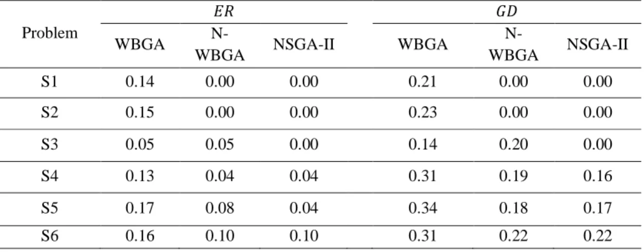
The results show that the proposed algorithm has a better performance in comparison to the WBGA but the NSGA-IIpresented the best results. According to table4, the number of non-dominance solution come out from the two algorithms N-WBGA and NSGA-II are approximately equal. Also table 5, shows that more than 90% solution of algorithms N-WBGA and NSGA-II are identical to the Pareto-optimal result.
150
Table 4. Comparison of the ONVG and ONVGR
Problem
Øœm× Øœmׯ
WBGA
N-WBGA NSGA-II WBGA
N-WBGA NSGA-II
S1 12 14 14 1 1 1
S2 13 13 13 1 1 1
S3 19 20 21 0.90 1 1
S4 22 22 22 0.87 1 1
S5 21 22 23 0.88 0.92 1
S6 26 28 28 0.84 0.90 0.90
Table 4. Comparison of the Error Ratio (ER) and Generational Distance (GD)
Problem
1¯ ×2
WBGA
N-WBGA NSGA-II WBGA
N-WBGA NSGA-II
S1 0.14 0.00 0.00 0.21 0.00 0.00
S2 0.15 0.00 0.00 0.23 0.00 0.00
S3 0.05 0.05 0.00 0.14 0.20 0.00
S4 0.13 0.04 0.04 0.31 0.19 0.16
S5 0.17 0.08 0.04 0.34 0.18 0.17
S6 0.16 0.10 0.10 0.31 0.22 0.22
5-2-2- Medium and large-sized problems
It is impossible or very time complexity for the medium and large-sized problems to find the Pareto-optimal solutions. Therefore, the comparison metrics which are used in the medium and large-sized problems must be restricted to indicators that don’t need to Pareto-optimal solutions. Hence, in this section two indicators Overall Non-dominated Vector Generation (ONVG) and Spacing (S) are used to evaluate performance of the proposed algorithm in solving the Medium and large-sized problems.
5-2-2-1- Overall Non-dominated Vector Generation (ONVG)
The Overall Non-dominated Vector generation (ONVG) as was explained in section 5.2.1.1., measures the total number of non-dominated vectors found during algorithm execution.
5-2-2-2- Spacing (S)
The spacing (S) metric numerically describes the spread of the vectors in PFe»¼½». In other word, this indicator measures the distance variance of neighboring vectors in PFe»¼½»as equation (35).
151
/ = Ù| .+JÔÕJ| − 1 × = ‚(1 * − (̅ƒ!
|•ÐÑ–ÒÓ–|
*4
[]` Z, = 1, 2, 3, … , (35)
Where (* indicates distances between the Z• solution from the nearest solution to it and is calculated as equation (36).
(* = 7Z ‚Û[*-)) − [ -))Û + Û[!*-)) − [!-))Ûƒ []` Z, = 1, 2, 3, … , (36)
In equation (32), f -x) and f!-x) can be supposed as the makespan and sum of earliness and tardiness in the considered problem.
Also dÝ is the mean of all dd and n is is the number of vectors in PFe»¼½».
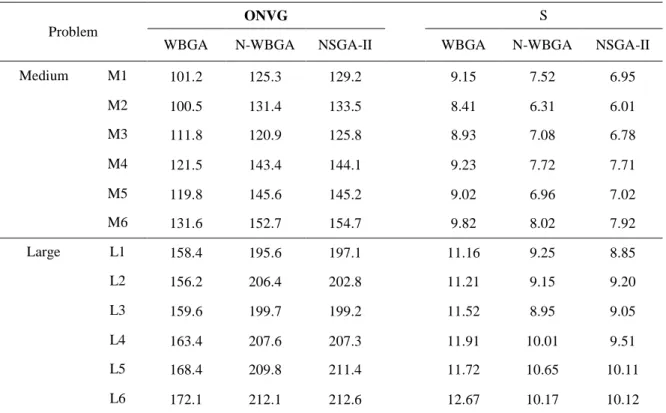
Table 6represents the average values of the two above mentioned metrics in medium and large problems. As illustrated in this table,the NSGA-II algorithm has the best performance. Also the proposed N-WBGA shows better performance than.
Table 6. Comparison of the Overall Non-dominated Vector Generation (ONVG) and Spacing (S)
Problem
ONVG S
WBGA N-WBGA NSGA-II WBGA N-WBGA NSGA-II
Medium M1 101.2 125.3 129.2 9.15 7.52 6.95
M2 100.5 131.4 133.5 8.41 6.31 6.01
M3 111.8 120.9 125.8 8.93 7.08 6.78
M4 121.5 143.4 144.1 9.23 7.72 7.71
M5 119.8 145.6 145.2 9.02 6.96 7.02
M6 131.6 152.7 154.7 9.82 8.02 7.92
Large L1 158.4 195.6 197.1 11.16 9.25 8.85
L2 156.2 206.4 202.8 11.21 9.15 9.20
L3 159.6 199.7 199.2 11.52 8.95 9.05
L4 163.4 207.6 207.3 11.91 10.01 9.51
L5 168.4 209.8 211.4 11.72 10.65 10.11
L6 172.1 212.1 212.6 12.67 10.17 10.12
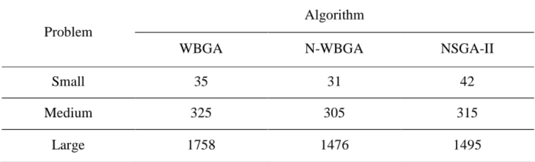
Table7 presents the average of computational times spent by algorithms after 10 generations executed in each test problem. As illustrated in this table, the proposed N-WBGA consumes less computational time than the others in all categories of problems. Because of the implemented structure of the calculations, the higher value of computationaltime of the NSGA-II is reasonableespecially for the small-sized problems.
152
Table 7. Run time of the algorithms
Problem
Algorithm
WBGA N-WBGA NSGA-II
Small 35 31 42
Medium 325 305 315
Large 1758 1476 1495
In total, the difference in computational time of two algorithms N-WBGA and NSGA-II is insignificant. So, the performance measures used in comparisons show that NSGA-II outperforms the other proposed algorithms.
6- Conclusion and future studies
In this paper a multi-objective scheduling problem was studied for a two-stage production system including a hybrid flow shop and an assembly stage.In this production system it is assumed that several products of differentkinds are ordered to be produced.The parts are manufactured in the hybrid flow shop and then the products are assembled in the assembly stage after preparing the parts. Two objective functions are considered simultaneously that are: (1) to minimizing the completion time of all products (makespan), and (2) minimizing the sum of earliness and tardiness of all products (∑ -Ed d∕ Td). Since this problem is NP-hard, a new multi-objective algorithm based on GA was designed for searching locally Pareto-optimal frontier for the problem. Various test problems were designed and the reliability of the proposed algorithm was presented in comparison two algorithms WBGA, and NSGA-II. The computational results show that the performance of the proposed algorithms is good in both efficiency and effectiveness.
For the future works, we recommend to address the problem with uncertain processing or setup times. Also considering this problem with a number of products of the samekind may be interestingas a future study. Consideringthe limitation in buffers is also suggested.
References
Allahverdi A, Al-AnziFS., (2009). The two-stage assembly scheduling problem to minimize total completion time with setup times. Computers & Operations Research 36: 2740-2747
Allahverdi, A., Aydilek, H., (2015). The two stage assembly flowshop scheduling problem to minimize total tardiness. Journal of Intelligent Manufacturing 26: 225-237.
Allahverdi, A., Aydilek H., Aydilek A., (2016). Two-Stage Assembly Scheduling Problem to Minimize Total Tardiness with Setup Times. Applied Mathematical Modelling 40: 7796-7815
Arroyo JAC, Armentano VA., (2005). Genetic local search for multi-objective flowshop scheduling problems. European Journal of Operational Research 167: 717–738
Cheng TCE, Wang G., (1999). Scheduling the fabrication and assembly of components in a two-machine flow shop. IIE Transactions 31:135-143
153
Coello CA, Lamont GB, Veldhuizen DAV., (2007).Evolutionary Algorithms for Solving Multi-Objective Problems. Second edition, Springer.
Ehrgott M., (2005).Multicriteria Optimization. Springer, Berlin, second edition, ISBN
Fattahi P, Hosseini SMH, Jolai F., (2012). A mathematical model and extension algorithm for assembly flexible flow shop scheduling problem. International Journal of Advance Manufacture Technology 65:787–802. DOI 10.1007/s00170-012-4217-x.
Fattahi, P., Hosseini, S.M.H., Jolai, F. and Tavakoli-Moghadam, R. (2014).A branch and bound algorithm for hybrid flow shop scheduling problem with setup time and assembly operations. Applied Mathematical Modelling. 38:119-134.
Fattahi, P., Hosseini, S.M.H., Jolai, F. and Safi-Samghabadi, A. (2014).Multi-objective scheduling problem in a threestage production system.International Journal of Industrial Engineering & Production Research.25:1-12.
Hariri AMA, Potts CN (1997). A branch and bound algorithm for the two-stage assembly scheduling problem. European Journal of Operational Research 103: 547-556
Jung s., Woo yb.,Soo Kim B., (2017). Two-stage assembly scheduling problem for processing products with dynamic component-sizes and a setup time. Computers & Industrial Engineering 104: 98–113 Karimi N, Zandieh M, Karamooz HR (2010). Bi-objective group scheduling in hybrid flexible flowshop: A multi-phase approach. Expert Systems with Applications 37: 4024–4032
Konak A, Coit DW, Smith AE (2006). Multi-objective optimization using genetic algorithms: A tutorial. Reliability Engineering and System Safety 91: 992–1007
KoulamasCh, Kyparisis GJ (2007). A note on the two-stage assembly flow shop scheduling problem with uniform parallel machines. European Journal of Operational Research 182: 945–951
Lee CY, Cheng TCE, Lin BMT (1993). Minimizing the makespan in the 3-machine assembly-type flowshop scheduling problem. Management Science 39: 616-625
Lin R, Liao ChJ (2012). A case study of batch scheduling for an assembly shop. International Journal of Production Economics 139: 473–483
Loukil T, Teghem J, Tuyttens D (2005). Solving multi-objective production scheduling problems using metaheuristics. European Journal of Operational Research 161: 42–61
Moslehi G, Mirzaee M, Vasei M, Modarres M, Azaron A (2009). Two-machine flow shop scheduling to minimize the sum of maximum earliness and tardiness. International Journal of Production Economics 122: 763–773
Potts CN, Sevast'Janov SV, Strusevich VA, Van Wassenhove LN, Zwaneveld CM (1995). The two-stage assembly scheduling problem: Complexity and approximation. Operations Research 43: 346-355
Rahimi-Vahed AR, Rabbani M, Tavakkoli-Moghaddam R, Torabi SA, Jolai F., (2007). A multi-objective scatter search for a mixed-model assembly line sequencing problem. Advanced Engineering Informatics 21: 85–99
154
Sukkerd, W. WuttipornpunT., (2016). Hybrid genetic algorithm and tabu search for finite capacity material requirement planning system in flexible flow shop with assembly operations. Computers & Industrial Engineering, 97: p. 157-169.
Sun Y, Zhang Ch, Gao L, Wang X., (2010). Multi-objective optimization algorithms for flow shop scheduling problem: a review and prospects. Int J AdvManufTechnol DOI 10.1007/s00170-010-3094-4 Sung CS, Kim Hah., (2008). A two-stage multiple-machine assembly scheduling problem for minimizing sum of completion times. International Journal of Production Economics 113: 1038-1048
Sup Sung Ch, Juhn J (2009). Makespan minimization for a 2-stage assembly scheduling problem subject to component available time constraint. International Journal of Production Economics 119: 392–401 Yokoyama M., (2001). Hybrid flow-shop scheduling with assembly operations. International Journal of Production Economics 73: 103-116
Yokoyama M, Santos DL (2005). Three-stage flow-shop scheduling with assembly operations to minimize the weighted sum of product completion times. European Journal of Operational Research 161: 754-770 Yokoyama M., (2008). Flow-shop scheduling with setup and assembly operations. European Journal of Operational Research 187: 1184–1195