Article
Epidemic Analysis of Wireless Rechargeable Sensor Networks
Based on an Attack–Defense Game Model
Guiyun Liu1 , Baihao Peng2,* and Xiaojing Zhong1
Citation: Liu, G.; Peng, B.; Zhong, X. Epidemic Analysis of Wireless Rechargeable Sensor Networks Based on an Attack–Defense Game Model. Sensors2021,21, 594.
https://doi.org/10.3390/s21020594
Received: 21 December 2020 Accepted: 12 January 2021 Published: 15 January 2021
Publisher’s Note:MDPI stays neu-tral with regard to jurisdictional clai-ms in published maps and institutio-nal affiliations.
Copyright: © 2021 by the authors. Licensee MDPI, Basel, Switzerland. This article is an open access article distributed under the terms and con-ditions of the Creative Commons At-tribution (CC BY) license (https:// creativecommons.org/licenses/by/ 4.0/).
1 School of Mechanical and Electric Engineering, Guangzhou University, Guangzhou 510006, China;
[email protected] (G.L.); [email protected] (X.Z.)
2 School of Electronics and Communication Engineering, Guangzhou University, Guangzhou 510006, China
* Correspondence: [email protected]
Abstract:Energy constraint hinders the popularization and development of wireless sensor networks (WSNs). As an emerging technology equipped with rechargeable batteries, wireless rechargeable sensor networks (WRSNs) are being widely accepted and recognized. In this paper, we research the security issues in WRSNs which need to be addressed urgently. After considering the charging process, the activating anti-malware program process, and the launching malicious attack process in the modeling, the susceptible–infected–anti-malware–low-energy–susceptible (SIALS) model is proposed. Through the method of epidemic dynamics, this paper analyzes the local and global stabilities of the SIALS model. Besides, this paper introduces a five-tuple attack–defense game model to further study the dynamic relationship between malware and WRSNs. By introducing a cost function and constructing a Hamiltonian function, the optimal strategies for malware and WRSNs are obtained based on the Pontryagin Maximum Principle. Furthermore, the simulation results show the validation of the proposed theories and reveal the influence of parameters on the infection. In detail, the Forward–Backward Sweep method is applied to solve the issues of convergence of co-state variables at terminal moment.
Keywords:wireless rechargeable sensor network; cyber security; stability analysis; optimal control
1. Introduction
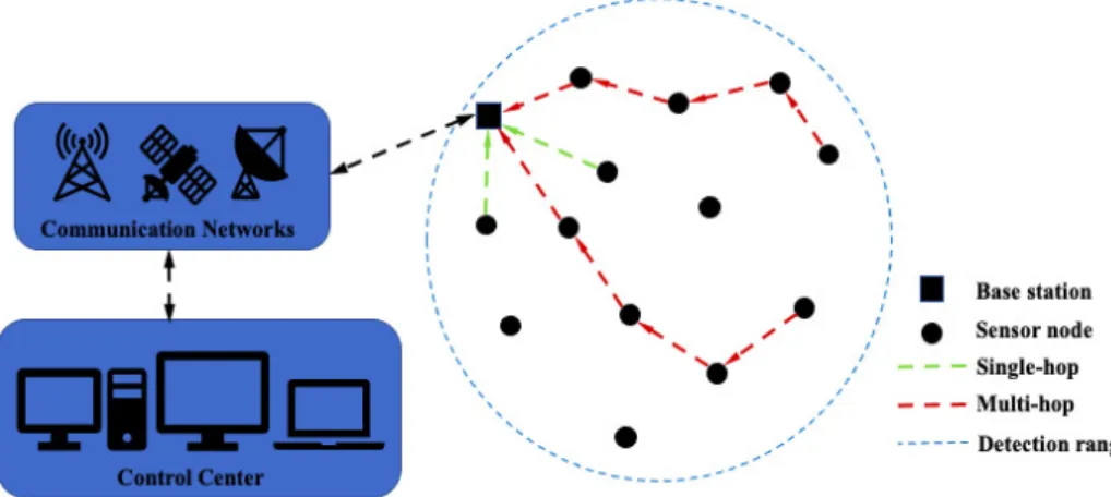
Wireless sensor networks (WSNs) are the research hotspot worldwide over the last few years [1–3]. Sensor nodes which serve the function of data storing and data transmitting capacities form WSNs in the way of multi-hop or single-hop, as depicted in Figure1. To monitor the physical parameters, such as temperature, humidity, pressure, etc., sensor nodes are randomly deployed in unattended areas. WSNs have widespread applications which are ranging from everyday life to various manufacturing industries [4]. However, due to the vulnerability of the sensor nodes and battery capacity limitations, the issues of security [5] and short lifespan [6] of WSNs are urgent to be tackled.
Focusing on optimizing energy utilization, scholars have proposed efficient schemes. However, comparing with the optimizing strategies, the operation of deploying recharge-able batteries can figure out the energy problem radically. Networks which are composed of rechargeable sensor nodes are named as wireless rechargeable sensor networks (WRSNs). Research hotspots on WRSNs mainly focus on solving the problems of both charging scheduling and system performance optimizations [7–9] in recent years. However, se-curity issues in WRSNs are seldom attracting the attention of scholars. Malware, as a self-replicating malicious code, can lead to network interruption and paralysis once it propagates in the networks. Even worse, rechargeable sensor nodes also suffer from the Denial of Charge (DOC) attacks [10]. Such attacks will cause catastrophic consequence to real-time and pre-warning application fields [11]. Thus, it is urgent to study the security of WRSNs based on the rechargeable characteristics.
For the past few years, some scholars have made contributions to security issues of WRSNs based on the characteristics of information transmission. Recent relevant studies are listed in Table1.
Figure 1.Communication architecture of wireless sensor networks. Table 1.Research on WRSN security.
Authors Problems Methods Results
A.N. Nguyen et al.
[12] Securing the physical layer
Time-switching power-splitting (TSPS) mechanism
The secrecy performance under TSPS is higher than the
traditional scheme J. Jung et al. [13]
Excessive energy consumption in the forward error correction(FEC)
method
Energy-aware FEC method
The developed method performs better than the former
one.
V.N. Vo et al. [14]
Securing energy harvesting wireless sensor networks(EH-WSNs) under
eavesdropping and signal interception
An optimization scheme that uses a
wirelessly powered friendly jammer The hypotheses are supported.
A. EI Shafie et al. [15]
Securing a single-antenna rechargeable source node in the
presence of a multi-antenna rechargeable cooperative jammer
and a potential single-antenna eavesdropper
An efficient scheme which can optimize the transmission times of
the source node
The average secrecy rate gain of the scheme is demonstrated
significantly
B. Bhushan et al. [16]
Securing the mobile sinks position information
Energy Efficient Secured Ring Routing (E2SR2) protocol
E2SR2 achieves improved performance than the existing
protocols
S. Lim et al. [17] Securing EH-WSNs under the Denial-of-Service (DoS) attacks
Hop-by-hop Cooperative Detection (HCD) scheme
HCD scheme can significantly reduce the number of forwarding misbehaviors and achieve higher packet delivery
ratio K J.S.R. Kommuru
et al. [18]
Balancing the trade-off between improving security and reducing
energy consumption
Low complexity XOR technique and Hybrid LEACH-PSO algorithm
The proposed approach performs better than the existing approaches. A. DI Mauro et al.
[19]
Securing the communications under energy constraints
Adaptive approach which allows nodes to dynamically choose the most appropriate parameters
Adaptive solution performs better
Table 1.Cont.
Authors Problems Methods Results
X. Hu et al. [20] Securing the up-link (UL) transmission
Establishing the communication model; deriving the energy outage
probabilities (EOP), connection outage probabilities (COP) and secrecy outage probabilities (SOP)
through comprehensive analysis
The theoretical derivations are verified
O. Bouachir et al. [21]
Securing the transmission between sensor nodes and base
stations
A novel strategy to select cluster heads and implement the non-orthogonal multiple access
(NOMA) technique in the transmission
The secrecy performance can be improved
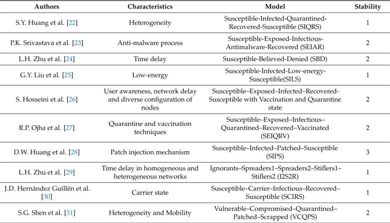
Due to the high similarity between infection mechanism of diseases in the population and the propagation mechanism of malware in WSNs, epidemic dynamics has also been widely used in the research of WSN security issues. In general, the applications of epidemic dynamics in WSNs mainly focus on the stability analysis of the built model. Recent relevant studies are listed in Table2.
Table 2.Research on stability of epidemic model in WSNs.
Authors Characteristics Model Stability
S.Y. Huang et al. [22] Heterogeneity
Susceptible-Infected-Quarantined-Recovered-Susceptible (SIQRS) 1 P.K. Srivastava et al. [23] Anti-malware process
Susceptible-Exposed-Infectious-Antimalware-Recovered (SEIAR) 2 L.H. Zhu et al. [24] Time delay Susceptible-Believed-Denied (SBD) 2
G.Y. Liu et al. [25] Low-energy
Susceptible-Infected-Low-energy-Susceptible(SILS) 1 S. Hosseini et al. [26]
User awareness, network delay and diverse configuration of
nodes
Susceptible–Exposed–Infected–Recovered-Susceptible with Vaccination and Quarantine
state
2
R.P. Ojha et al. [27] Quarantine and vaccination techniques
Susceptible–Exposed–Infectious– Quarantined–Recovered–Vaccinated
(SEIQRV)
2
D.W. Huang et al. [28] Patch injection mechanism Susceptible–Infected–Patched–Susceptible
(SIPS) 3
L.H. Zhu et al. [29] Time delay in homogeneous and heterogeneous networks
Ignorants–Spreaders1–Spreaders2–Stiflers1–
Stiflers2 (I2S2R) 1 J.D. Hernández Guillén et al.
[30] Carrier state
Susceptible–Carrier–Infectious–Recovered–
Susceptible (SCIRS) 1 S.G. Shen et al. [31] Heterogeneity and Mobility Vulnerable–Compromised–Quarantined–
Patched–Scrapped (VCQPS) 2 1: Local and global stability in malware-free and epidemic points; 2: Local and global stability in malware/rumor/worm-free point; 3: local and global stability in epidemic point.
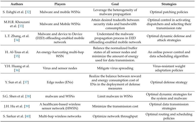
Although the above models consider the characteristics of WSNs from various aspects, they do not analyze and model the networks based on the energy level. Besides, to our knowledge, the studies combining epidemic dynamics with WRSNs are very few. Therefore, this paper divides sensor nodes in WRSNs according to the residual energy and infection of sensor nodes and introduces the charging process. Differential games are also widely used in WSNs as a method of studying optimal dynamic strategies. Recent relevant studies are listed in Table3.
Table 3.Research on differential game applied in WSNs.
Authors Players Goal Strategies
S. Eshghi et al. [32] Malware and mobile WSNs Leverage the heterogeneity of
malware propagation Optimal patching policies M.H.R. Khouzani
et al. [33] Malware and Mobile WSNs
Attain desired tradeoffs between security risks and bandwidth
consumption
Optimal control in activating dispatchers and selecting their
transmission rate L.T. Zhang, et al.
[34]
Malware and device to Device (D2D) offloading-enabled mobile
network
Understand the malware propagation process in D2D offloading-enabled mobile network
Optimal dynamic defense and attack strategies
H. Al-Tous et al. [35]
An energy-harvesting multi-hop WSN
Balance the normalized buffer states of all sensor nodes and minimize the amount of energy
used for data transmission.
An online power control and data scheduling algorithm Y.H. Huang et al.
[36] Virus and sensor nodes Mitigate virus spreading
Virus-resistant weight adaptation policies
Y. Sun et al. [37] Edge nodes (ENs)
Realize the balance between reward and energy consumption cost of ENs in the deployment of defense
measures
Optimal defense strategy
S.G. Shen et al. [38] malware and WSNs Limit malware in WSNs Optimal dynamic strategies for the system and malware J.H. Hu et al. [39] A healthcare-based wireless
sensor network (HWSN) Minimize the transmission cost
Optimal data transmission strategies
S. Sarkar et al. [40] Multi-hop wireless networks Optimize network throughput Optimal routing and scheduling policies
Based on the previous works [41] and inspired by [23], this paper proposes an epidemic model that includes the anti-malware (A) state, constructs game between malware and WRSNs, and obtains the optimal control strategies for both parties.
In the research on the security of WRSNs, few scholars analyze the issues by applying the relevant knowledge of epidemic dynamics. By establishing the dynamic differential equations of the propagation of malware in WRSNs, both the propagation mechanism of malware and the defense mechanism of WRSNs can be dynamically understood so as to provide novel thoughts and directions for resisting the invasion of malware.
In this paper, a susceptible infected anti-malware low-energy susceptible (SIALS) model is proposed by considering the charging process and the process of activating of the anti-malware program.The SIALS model can not only reflect the infection in WRSNs but also reveal the trend of the residual energy of the sensor nodes. At the same time, to describe the attack modes of malware, this paper considers the hardware attacks launched by malware and charging process compromised with malware.
Additionally, through the theory of stability analysis, the local and global stabilities of the disease-free equilibrium point and the epidemic equilibrium point of SIALS model are proved. Furthermore, this paper analyzes the game composed of malware and WRSNs by applying the Pontryagin Maximum Principle and obtains the optimal control strategies. Consequently, this work enriches the application of epidemic dynamics and differential games in addressing the security issues on WRSNs.
The rest of the paper is organized as follows. The introduction of the modeling of SIALS is presented in Section2. Theorems of the local and global stability and the optimal strategies are proved in Section3. The simulation results are shown in Section4. The conclusions are drawn in Section5.
2. Modeling
2.1. Dynamic Equation
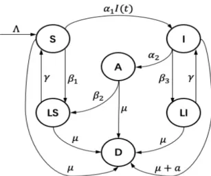
In this paper, WRSNs consist of homogeneous rechargeable nodes which are randomly distributed. Meanwhile, the number of nodes increase at rate Λ, where Λis greater than 0. Suppose that nodes in the networks belong to one of six possible compartment: susceptible (S), infected (I), anti-malware (A), low-energy and susceptible (LS), low-energy and infected (LI), and dysfunction (D). The relationship between the six compartments are depicted in Figure2.Snodes are vulnerable to malware;Inodes are compromised with attacker;Anodes clear malware by activating anti-malware program;LSandLI nodes are both in low-energy level and remain dormant; andDnodes are totally out of function. Now, let us impose a set of hypotheses as follows.
Figure 2.Flow diagram of the improved epidemic model.
(a) Malware propagates by broadcasting. Assuming that the ratio ofInodes successfully infectingSnodes isα1S(t), whereα1is greater than 0, then the proportion of the new
infected in the network isα1S(t)I(t).
(b) Considering mobile chargers and rechargeable modules, after the nodes in Adrop toLSatβ2, anti-malware programs stop running, and the nodes return toSat rateγ
when they are fully charged.β2andγare all greater than 0.
(c) Nodes inS,I, andAdrop to low-energy level at different ratiosβ1,β3, andβ2, where
β1 < β2 <β3. Among them, owing to the running of anti-malware program,β2is
greater thanβ1. Due to the software attack launched by malware,β3is greater than
β1andβ2.β1,β2, andβ3are all greater than 0.
(d) Suppose that, except forI, the four remaining compartmentsS,A,LS, andLI have the same mortalityµ.Iis different in that malware also launches hardware attacks at
rateato cause damage.µandaare all greater than 0.
(e) Regardless of other protective measures, this paper only considers activating anti-malware program to achieve the purpose of clearing anti-malware temporarily.
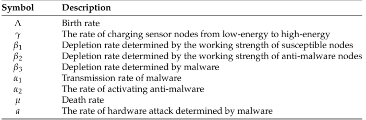
Table 4.Epidemiological coefficients of the model. Symbol Description
Λ Birth rate
γ The rate of charging sensor nodes from low-energy to high-energy β1 Depletion rate determined by the working strength of susceptible nodes
β2 Depletion rate determined by the working strength of anti-malware nodes
β3 Depletion rate determined by malware
α1 Transmission rate of malware
α2 The rate of activating anti-malware
µ Death rate
a The rate of hardware attack determined by malware
On the basis of the above hypotheses, a novel dynamical system is obtained in (1)–(6): ˙ S(t) =Λ−(α1I(t) +β1+µ)S(t) +γLS(t), (1) ˙ I(t) =α1S(t)I(t)−(α2+β3+µ+a)I(t) +γLI(t), (2) ˙ A(t) =−(β2+µ)A(t) +α2I(t), (3) ˙ LI(t) =−(γ+µ)LI(t) +β3I(t), (4) ˙ LS(t) =−(γ+µ)LS(t) +β1S(t) +β2A(t), (5) and ˙ D(t) =µN(t) +aI(t), (6) whereN(t) =S(t) +I(t) +A(t) +LS(t) +LI(t)and ˙ N(t) =Λ−µN(t)−aI(t). (7)
2.2. Computation of the Steady States and the Basic Reproductive Number
ConsideringLS(t) =N(t)−S(t)−I(t)−A(t)−LI(t), (1) can be rewritten as
˙
S(t) =Λ−(α1I(t) +β1+µ)S(t) +γ(N−S(t)−I(t)−A(t)−LI(t)), (8)
whereN(t) =N(∞) = Λ−aI(t)
µ .
Then, the solutions of the limit system (8) and (2)–(4) are the steady states of the system (1)–(5).
The first solution is the disease-free steady state:E0= (S0,I0,A0,LI0), whereI0=0, A0=0,LI0=0, and
S0= Λ
(µ+γ)
(µ+γ)(µ+β1)−γβ1
. (9)
The second solution is the epidemic steady stateE∗= (S∗,I∗,A∗,LI∗), and
S∗= (α2+β3+µ+a)(γ+µ)−γβ3
α1(γ+µ) , (10)
I∗= ∆1+γΛ(β2+µ)(γ+µ)
A∗= α2∆1+α2γΛ(β2+µ)(γ+µ) (β2+µ)(∆2+∆3) , (12) and LI∗= β3∆1+β3γΛ(β2+µ)(γ+µ) (γ+µ)(∆2+∆3) , (13) where ∆1= [Λ−(β1+µ+γ)S∗][µ(β2+µ)(γ+µ)], (14) ∆2=µ(β2+µ)(γ+µ)[γ+α1S∗], (15) and ∆3=γ[a(β2+µ)(γ+µ) +α2µ(γ+µ) +β3µ(β2+µ)]. (16)
Consequently, considering the next generation matrix method, the basic reproductive numberR0is its spectral radius.
Set F= α1S(t) 0 0 0 (17) and V= α2+β3+µ+a −γ −β3 γ+µ . (18) Thus, R0=F·V−1= α1S0(γ+µ) (α2+β3+µ+a)(γ+µ)−γβ3 = α1Λ(γ+µ) 2 [(β1+µ)(γ+µ)−γβ1][(α2+β3+µ+a)(γ+µ)−γβ3] . (19)
3. Dynamic Analysis and Optimal Strategy
In this section, the stability and the optimal strategy in the SIALS model are discussed. In Section3.1, the local and global stabilities of the disease-free point are proved by using the eigenvalues and the Lyaponov function. In Section3.2, the local and global stabilities of the epidemic point are proved by using the Routh criterion and Bendixson-Dulac criterion. In Section3.3, a five-tuple attack–defense game is proposed and the optimal strategies of malware and WRSNs are obtained by applying the Pontryagin Maximum Principle. 3.1. Analysis of Disease-Free Equilibrium Point
Theorem 1. The disease-free equilibrium point, E0, is locally asymptotically stable if R0<1. Proof. Here, we use matrix eigenvalues to verify the validity of the theorem. In general, if the eigenvalues of the system matrix are negative, then the system must be stable.
Consider the follow matrix F−V= α1S0−(α2+β3+µ+a) γ β3 −γ−µ (20) The eigenvalues of (20) are
λ1=0.5(−B1+ q B21+4B2) (21) and λ2=0.5(−B1− q B12+4B2), (22)
whereB1 = (γ+µ)−[α1S0−(α2+µ+β3+a)]andB2 = [(µ+γ)(α2+β3+µ+a)− γβ3](R0−1). The real parts of the two eigenvalues are negative ifR0<1. Besides,
∂(Λ−(β1+µ)S(t) +γ(N−S))
∂S =−β1−µ−γ<0. (23)
Thus,E0is locally asymptotically stable [42] whenR0 <1. Conversely,E0is unstable if R0>1.
Theorem 2. The disease-free equilibrium point, E0, is globally asymptotically stable if R0≤1. Proof. Here, Lyapunov stability method is applied. In general, a positive definite Lyaponov function with negative definite first derivative needs to be established to test the stability of the system [43]. Considering a Lyaponov functionV(t) = (γ+µ)I(t) +γLI(t)>0, we
have: ˙ V(t) = (γ+µ)I(˙t) +γLI˙(t) ≤I(t)[(γ+µ)α1S0−(γ+µ)(α2+β3+µ+a) +γβ3] = (γ+µ)[α1S0I(t)−(α2+β3+µ+a)I(t)] +γβ3I(t) =I(t)[(γ+µ)α1S0−(γ+µ)(α2+β3+µ+a) +γβ3] ≤I(t)(R0−1) (24) In addition,dV
dt =0 if and only ifR0=1 andI(t) =0. Moreover, (S,I,A,LI) tends to E0whenttends to infinity, and the maximum invariant set in{(S,I,A,LI)∈Ω:
dV dt =0} is E0. Thus, Theorem2 is proved, after considering the La-Salle Invariance Principle
[44].
3.2. Analysis of Epidemic Equilibrium Point
Theorem 3. The epidemic equilibrium point, E∗, is locally asymptotically stable if R0>1. Proof. Here, the Routh criterion is applied to prove the theorem. Firstly, the Jacobian matrix of the limit system is:
−(α1I(t) +β1+µ)−γ −α1S(t)−γ− aγ µ −γ −γ α1I(t) α1S(t)−(α2+β3+µ+a) 0 γ 0 α2 −(β2+µ) 0 0 β3 0 −(γ+µ) (25)
Then, the characteristic polynomial of (25) inE∗is
P(λ) =P1λ4+P2λ3+P3λ2+P4λ1+P5, (26) where P1=1>0, (27) P2=a+β1+α2+β2+β3+2γ+4µ+α1θ3(R0−1) + γβ3 γ+µ >0, (28) P3= (β2+µ) γβ3 γ+µ+α1(α1S ∗+ γ)θ3(R0−1) + (γ+µ)(β2+µ+ γβ3 γ+µ) +θ1(θ2+ γβ3 γ+µ)>0, (29)
P4= (γ+µ)(β2+µ) γβ2 γ+µ+α1θ3(R0−1)(α1S ∗ +γ)(β2+µ)θ2+θ1[(γ+µ)(β2+µ) +θ2 γβ3 γ+µ]>0, (30) and P5=α1θ3(R0−1)(α1S∗+γ)(γ+µ)(β2+µ)>0, (31) where θ1=α1I∗+β1+µ+γ, (32) θ2=γ+2µ+β2, (33) and θ3= β2+µ α1(γ+µ)[(α2+β3+µ+a) +γµ(β2+µ) +aγ(β2+µ) +α2γµ] (34)
Moreover, a simple calculation showsP2P3−P1P4>0 andP2P3P4−P1P42−P22P5>0.
Thus, ifR0>1, applying the Routh criterion [45], the local asymptotically stability ofE∗is
tenable.
Theorem 4. The epidemic equilibrium point, E∗, is globally asymptotically stable if R0≥1. Proof. Set D(I,LI) = 1 ILI, (35) P=α1S(t)I(t)−(α2+β2+µ+a)I(t) +γLI(t), (36) and Q=−(γ+µ)LI(t) +β3I(t). (37)
Considering the following formulation:
∂(DP) ∂I + ∂(DQ) ∂LI =−γI −2− β3LI−2<0 (38)
By applying the Bendixson–Dulac criterion [46], the system admits no periodic orbits in the interior ofΩ.
Let (I, LI) be a smooth point on the boundary ofΩ. Along the boundary, there exists two possibilities:
(a) 0≤ I<1,LI=0. Then, dP(t)
dt =β3I(t)≥0. The value 0 occurs if and only ifI=0. (b) 0 ≤ LI < 1, I = 0. Then, dQ(t)
dt = γLI(t) ≥ 0. The value 0 occurs if and only if LI =0.
Thus, there is no periodic solutions that pass through the boundary.
In view of Theorem3, the claim follows from the generalized Poincare–Bendixson theorem [46].
3.3. Optimal Strategies
Based on the evolution of node state during the confrontation between malware and WRSNs, an attack–defense game model is constructed as follows.
The attack–defense game based on the SIALS model can be expressed as a five-tuple
G={P,ν,µ,X,Λ}, where
• P={PA,PD}is the set of plays in the attack–defense game. PAis the attacker andPD is the defender.
• ν = {ASI(t),ALI I(t),AID(t)} is a set of strategies implemented by the malware. ASI(t)represents the spreading capability of the malware, ALI I(t)represents the strength of the attacks on the charging process, andAID(t)represents the strength of the hardware attack. In particular, the three control strategies are all constrained by the upper and lower bounds.
• µ={DI A(t),DLSS(t)}is a set of strategies implemented by the WRSNs.DI A(t) rep-resents the strength of activation of the anti-malware program andDLSS(t)represents the control of the charging process by WRSNs. Similarly, the two strategies have upper and lower bounds.
• X = {X(t)|S(t),I(t),A(t),LS(t),LI(t),D(t)}is a set of the state variables on the SIALS model. The denotations of the state variables are the same as the statement in Section2.1.
• Λ={Λ(t)|λS(t),λI(t),λA(t),λLS(t),λLI(t),λD(t)}is a set of the adjoint variables of the games
Considering the controlled process stated above, (1)–(6) transform to ˙ S(t) =Λ−(α1ASI(t)I(t) +β1+µ)S(t) +γDLSS(t)LS(t), (39) ˙ I(t) =α1ASI(t)S(t)I(t)−(α2DI A(t) +β3+µ+aAID(t))I(t) +γALI I(t)LI(t), (40) ˙ A(t) =−(β2+µ)A(t) +α2DI A(t)I(t), (41) ˙ LS(t) =−(γDLSS(t) +µ)LS(t) +β1S(t) +β2A(t), (42) ˙ LI(t) =−(γALI I(t) +µ)LI(t) +β3I(t), (43) and ˙ D(t) =µN(t) +aAID(t)I(t). (44) In this paper, we mainly focus on how to effectively suppress the growth of malware. Furthermore, in the purpose of maintaining the operation of the networks, the phenomenon of network interruption and paralysis caused by the dysfunctionality of the sensor nodes need to be minimized. Therefore, the number of the infected and dysfunctional sensor nodes is used to measure the overall cost in the attack–defense game. SetJ(·)as the overall cost of the game and
J(X(t),µ(t),ν(t)) = Z tf
t0
{CII(t) +CDD(t)}dt. (45) The above description of the cost index is a classic Lagrange problem in differential games. In (6),t0andtf, respectively, represent the initial and terminal moment of the game. Specifically,CII(t)is the instantaneous cost determined by the damage capability and the number ofInodes at timet, whereCI>0.CDD(t)is the instantaneous cost determined by the impact of network interruption and paralysis at timet, whereCD>0.
In this game, the goal of both parties is to influence changes in the costJ(·)to make it more beneficial to their own development. Malware aims to maximizeJ(·), while WRSNs aim to minimizeJ(·). Therefore, malware needs to apply the dynamic strategies inν(t)to
maximizeJ(·)and WRSNs need to use the dynamic strategies inµ(t)to minimize theJ(·).
To achieve the purpose of both parties, Theorem5is given by applying the Pontryagin Maximum Principle.
Theorem 5. Based on the state functions (39)–(44), there exist an optimal strategy set{µ∗(t), ν∗(t)}={(D∗I A(t),D∗LSS(t)),(A∗SI(t),A∗ID(t),A∗LI I(t))}in the attack–defense game such that
J(X(t),µ∗(t),ν∗(t)) =maxνminµJ(X(t),µ(t),ν(t)) =minµmaxνJ(X(t),µ(t),ν(t)). (46) The expressions of the optimal strategies are
A∗SI(t) = maxASI, (λI(t)−λS(t))α1S(t)I(t)>0 minASI, (λI(t)−λS(t))α1S(t)I(t)<0, (47) A∗ID(t) = maxAID, (λD(t)−λI(t))aI(t)>0 minAID, (λD(t)−λI(t))aI(t)<0, (48) A∗LI I(t) = maxALI I, (λI(t)−λLI(t))γLI(t) +CCγLI(t)>0 minALI I, (λI(t)−λLI(t))γLI(t) +CCγLI(t)<0, (49) D∗I A(t) = minDI A, (λA(t)−λI(t))α2I(t)>0 maxDI A, (λA(t)−λI(t))α2I(t)<0, (50) and D∗LSS(t) = minDLSS, (λS(t)−λLS(t))γLS(t) +CCγLS(t)>0 maxDLSS, (λS(t)−λLS(t))γLS(t) + +CCγLS(t)<0. (51)
Proof. First, there exists a saddle-point in the game according to [41].
Then, in view of (39)–(44) and (45), the Hamiltonian function constructs as:
H(X(t),λ(t),µ(t),ν(t),t) =λS(t)S(˙t) +λI(t)I(˙t) +λA(t)A(˙t) +λLS(t)LS˙(t) +λLI(t)LI˙(t) +λD(t)D(˙t) +CII(t) +CDD(t)
(52) Note that the constraints of the adjoint variables are given by the following formulas [44]: ˙ λS(t) = (λS(t)−λI(t))α1ASI(t)I(t) + (λS(t)−λLS(t))β1+ (λS(t)−λD(t))µ, (53) ˙ λI(t) =(λS(t)−λI(t))α1ASI(t)S(t) + (λI(t)−λA(t))α2DI A(t) + (λI(t)−λLI(t))β3+ (λI(t)−λD(t))(µ+aAID(t))−CI, (54) ˙ λA(t) = (λA(t)−λLS(t))β2+ (λA(t)−λD(t))µ, (55) ˙ λLS(t) = (λLS(t)−λS(t))γDLSS(t) + (λLS(t)−λD(t))µ, (56) ˙ λLI(t) = (λLI(t)−λI(t))γALI I(t) + (λLI(t)−λD(t))µ, (57) and ˙ λD(t) =−CD. (58)
Furthermore, the end values of the adjoint variables all equal to 0, i.e.,
λSt f =λIt f =λAt f =λLSt f =λLIt f =0. (59)
Finally, according to the Pontryagin Maximum Principle, the optimal strategies are obtained by
As a consequence, in the optimal case, when(λI(t)−λS(t))α1S(t)I(t)>0, the malware
exerts the maximum effort to infect vulnerable sensor nodes; otherwise, it does not propa-gate. When(λD(t)−λI(t))aI(t)>0, the malware exerts the maximum effort to launch the hardware attack; otherwise, it does nothing in hardware equipped in sensor nodes. When(λI(t)−λLI(t))γLI(t) +CCγLI(t)<0, the malware exerts the minimum effort to
influence the charging process toLInodes; otherwise, theLInodes accept the charging requests. Moreover, when(λA(t)−λI(t))α2I(t)<0, WRSNs exist the maximum effort to
clear the malware; otherwise, the networks do nothing in activating anti-malware program. When(λS(t)−λLS(t))γLS(t) +CCγLS(t)<0, WRSNs exist the maximum effort to charge
theLSnodes; otherwise,LSnodes do not be charged.
4. Simulation
The purpose of this section is to further verify and develop the theorems stated in Section3. In detail, the first three subsections focus on the stability of the system (1)–(6) and the last three subsections focus on the optimal control of the system (39)–(44).
The parameters used in the simulations were set as:Λ=0.2,α1=0.0001,α2=0.001,
β1 =0.005,β2 =0.005,β3=0.008,µ=0.004,a=0.005, andγ =0.05. All simulations
were run on MacOS Catalina (Intel Core i5, 8GB, 1.8GHz) and MATLAB 2017b. 4.1. Stable Analysis When R0<1
In this subsection, the stability of the system (1)–(6) is verified whenR0 <1.
Sub-stituting the parameters into (19), we obtainedR0 = 0.432 < 1. Thus, there must exist
a disease-free equilibrium point (S0,I0,A0,LS0,LI0) in the system. According to (10), S0=45.76,I0=0,A0=0,LS0=4.23, andLI0=0. The simulation results are illustrated
in Figure3.
For the purpose of showing the changing trend of the system in a more three-dimensional and comprehensive way, we consider to verify the stability of the system in the form of three dimensions. We setN(t)≤50 (i.e.,S(t) +I(t) +A(t) +LS(t) +LI(t)≤50). Therefore, in the case of three dimensions, the feasible region is a regular triangular pyra-mid with an equilateral triangle at its base and a right-angled isosceles triangle (Waist = 50) at its three sides.
The curves in Figure3a,c,e all begin from the axes and the curves in Figure3b,d,f all start at the boundary on the hypotenuses.
As shown in Figure3a,b, in the three-dimensional area formed by the number ofA nodes as the x-axis, the number ofInodes as the y-axis, and the number ofSnodes as the z-axis, the curves eventually converge to(0, 0, 45.67)from the six boundaries. In detail, in Figure3a, when the curves start from x-axis, it is assumed that that there exists onlyAand LInodes in the networks at the initial moment; when the curve starts from the z-axis, it is assumed that that onlySandLInodes in the network at the initial moment; and when the curve starts from y-axis, it is assumed that that onlyIandLSnodes in the network at the initial moment. The purpose of these assumptions is to ensure that malware exists in the network at the beginning, otherwise it would be meaningless. In Figure3b, in theS-A plane, we set the sum ofSnodes andAnodes as 49, and the number ofLInodes as 1 at the beginning. In theS-Iplane, we set the sum of the number ofSandInodes as 50 at the beginning. In theA-Iplane, we set that the sum of the number ofAandInodes is 50 at the beginning.
Similarly, in the three-dimensional area formed by the number ofLI nodes as the x-axis, the number ofInodes as the y-axis, and the number ofSnodes as the z-axis, the curves eventually converge to(0, 0, 45.67), as shown in Figure3c,d. Here, the principle of assumption is the same as above. The curves start from y-axis contain onlyIandLSnodes at the beginning. The curves start from the x-axis initially contain onlyLIandLSnodes at the beginning. It is worth noting that, in Figure3c, the curve starts from the z-axis is reunited with the z-axis because it does not contain malware at the beginning. In Figure3d,
the curves start from theS-LIplane initially contain onlySandLInodes; the curves start from theS-Iplane initially contain onlySandInodes; and the curves start from theI-LI plane initially contain only I and LI nodes.
0 0 10 20 0 S nodes 30 20 10 I nodes 40 20 A nodes 50 30 40 40 50 (0, 0, 45.76)
(a)The number of S, I, and A nodes (Begin from coordinate axes)
0 0 10 20 0 S nodes 30 20 10 I nodes 40 20 A nodes 50 30 40 40 50 (0, 0, 45.76)
(b)The number of S, I, and A nodes (Begin from the hypotenuses)
0 0 10 20 0 S nodes 30 20 10 I nodes 40 20 LI nodes 50 30 40 40 50 (0, 0, 45.76)
(c)The number of S, I, and LI nodes (Begin from coordinate axes)
0 0 10 20 0 S nodes 30 20 10 I nodes 40 20 LI nodes 50 30 40 40 50 (0, 0, 45.76)
(d)The number of S, I, and LI nodes (Begin from the hypotenuses)
0 0 10 20 0 S nodes 30 20 10 A nodes 40 20 LS nodes 50 30 40 40 50 (4.23, 0, 45.76)
(e)The number of S, A, and LS nodes (Begin from coordinate axes)
0 0 10 20 0 S nodes 30 20 10 A nodes 40 20 LS nodes 50 30 40 40 50 (4.23, 0, 45.76)
(f)The number of S, A, and LS nodes (Begin from the hypotenuses)
In the three-dimensional area formed by the number ofLSnodes as the x-axis, the number of Anods as the y-axis, and the number of S nodes as the z-axis, the curves eventually converge to(4.23, 0, 45.76), as shown in Figure3e,f. Similarly, in Figure3e, the curves begin from the z-axis initially containSandI nodes; the curves begin from the x-axis initially containLSandInodes; and the curves begin from the y-axis initially contain AandInodes. In Figure3f, the curves begin fromS-Aplane initially containS,A, and Inodes, and the sum of the number ofSandAnodes are 49 and the number ofInodes is 1; the curves begin fromS-LSplane initially containS,LS, andInodes, and the sum of the number ofSandLSnodes are 49 and the number ofInodes is 1; and the curves begin fromA-LSplane initially containA,LS, andInodes, and the sum of the number ofAand LSnodes are 49 and the number of Inodes is 1.
In Figure3a–d, when the initial number ofInodes is less than a threshold, the number ofInodes has a peak value and decreases after that, and finally reaches 0. When the number ofInodes is greater than this threshold, the number ofInodes decreases continuously because the number of newly infected nodes is smaller than the number of newly recovered nodes. All these results confirm Theorems1and2.
4.2. Stable Analysis When R0>1
In this subsection, the situation underR0 > 1 is discussed. Except forα1 = 0.001,
the parameters remain the same as above. In this simulation,R0=4.320>1,S∗ =10.59, I∗ = 15.25, A∗ =1.69, LS∗ = 1.13, LI∗ = 2.25 andN(∞) = 30.9375 based on (10)–(13) and (19). As in the Section4.2, supposeN(t)≤50. The simulation results are shown in Figure4.
The assumptions at the initial moment of the curve in this subsection are the same as in Section4.1. As shown in Figure4a,b, in the three-dimensional area formed by the number of Anodes as the x-axis, the number ofInodes as the y-axis, and the number ofSnodes as the z-axis, the curves eventually converge to(1.69, 15.25, 10.59)from the boundaries at the axes and the hypotenuses. In the three-dimensional area formed by the number ofLInodes as the x-axis, the number of Inodes as the y-axis, and the number ofSnodes as the z-axis, the curves eventually converge to(2.25, 15.25, 10.59)from the boundaries, as shown in Figure4c,d. In the three-dimensional area formed by the number ofLSnodes as the x-axis, the number ofAnodes as the y-axis, and the number ofSnodes as the z-axis, the curves eventually converge to(1.13, 1.69, 10.59)from the boundaries, as shown in Figure4e,f. All these results confirm Theorems3and4.
Compared with the case ofR0<1, more peaks exist in the process of quantity change
whenR0>1, but the general trend is similar. ForInodes, when the initial number is less
than a certain threshold, it peaks and then eventually stabilize at the steady state value. When the initial number is greater than this threshold, the number ofInodes continues to decline until the steady state value. It is worth noting that the trend of the number of nodes is affected by the initial value. The trend changes if the initial values are set differently. However, if the model parameters do not change, the final value of the number of nodes does not change.
0 0 10 20 0 S nodes 30 20 10 I nodes 40 20 A nodes 50 30 40 40 50 (1.69, 15.25, 10.59)
(a)The number of S, I, and A nodes (Begin from coordinate axes)
0 0 10 20 0 S nodes 30 20 10 I nodes 40 20 A nodes 50 30 40 40 50 (1.69, 15.25, 10.59)
(b)The number of S, I, and A nodes (Begin from the hypotenuses)
0 0 10 20 0 S nodes 30 20 10 I nodes 40 20 LI nodes 50 30 40 40 50 (2.25, 15.25, 10.59)
(c)The number of S, I, and LI nodes (Begins from coordinate axes)
0 0 10 20 0 S nodes 30 20 10 I nodes 40 20 LI nodes 50 30 40 40 50 (2.25, 15.25, 10.59)
(d)The number of S, I, and LI nodes (Begin from the hypotenuses)
0 0 10 20 0 S nodes 30 20 10 A nodes 40 20 LS nodes 50 30 40 40 50 (1.13, 1.69, 10.59)
(e)The number of S, A, and LS nodes (Begins from coordinate axes)
0 0 10 20 0 S nodes 30 20 10 A nodes 40 20 LS nodes 50 30 40 40 50 (1.13, 1.69, 10.59)
(f)The number of S, A, and LS nodes (Begin from the hypotenuses)
4.3. Influence of Parameters under Stable State
In this subsection, the influence of parameters on the spread of malware is analyzed. In detail, we analyzed the influence ofα1,α2,β3, andγon the number of I nodes. The
values ofα1,α2, andβ3range from 0.0001 to 0.01, and the value ofγranges from 0.01 to 1.
Figure5a shows the relationship betweenα1andα2and the number ofInodes when t→∞. Figure5a shows that, by reducing the transmission rateα1, malware can eventually
be cleared. At the same time, increasing the removal rateα2of malware can effectively
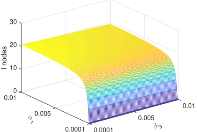
suppress the increasing of malware; Figure5b shows the relationship betweenα1andβ3
and the number ofInodes whent→∞. As shown in Figure5b, the behavior of malware to drops nodes toLIstate by increasing the frequency or intensity of exhaustion attacks cannot be too effective to increase the number ofInodes in the steady state. Figure5c shows the relationship betweenγandα2and the number ofInodes in steady state. Figure5c clearly
shows that controlling the frequency or power of chargingγcan restrain the spread of
malware to a certain extent. Figure5d shows the relationship betweenγandβ3and the
number ofInodes in the steady state. As shown in Figure5d, increasing the intensity of software attacks has little effect on the eventual prevalence of malware. On the contrary, when the charging rate γ drops to a certain extent, the amount of malware is greatly
reduced. This suggests that we can control the charging rateγto suppress the spread of
malware. Figure5e shows the relationship betweenβ3andα2and the number ofInodes in
the steady state. In Figure5e, the influence ofβ3on the eventual prevalence of malware is
verified again. At the same time, the effect of increasing the rate of activating anti-malware programs on the prevalence of malware is more obvious. Figure5f shows the relationship betweenα1andγand the number ofInodes in the steady state. As shown in Figure5f, the
method of reducing the number ofInodes by reducing the charging rate and transmission rate is verified again.
Among them, the most effective suppression method is to reduce the transmission rateα1. By increasing removal rateα2and reducing the charging rateγ, the number of
malware can be reduced to a certain extent whent→∞. In detail, although the method of reducing the transmission rate has a good effect, the effect is obvious when it is reduced to a certain extent, which is impractical in real life. The most direct method is to activate the anti-malware program to remove its own malware. The method of charging control is similar to the method of adjusting the transmission rate, which needs to be reduced to a certain threshold before the effect becomes obvious. Therefore, the method of suppressing malware by adjusting the transmission rate and charging rate is effective but requires much more consideration than activating the ant-malware program.
0 0.01 10 0.01 I nodes 20 1 0.005 2 30 0.005 0.0001 0.0001
(a)Variation trend under variousα1andα2
0 0.01 10 0.01 I nodes 20 1 0.005 3 30 0.005 0.0001 0.0001
(b)Variation trend under variousα1andβ3
0 1 5 0.01 10 I nodes 15 0.05 2 20 0.005 0.01 0.0001
(c)Variation trend under variousγandα2
10 1 12 0.01 14 I nodes 16 0.05 3 18 0.005 0.01 0.0001
(d)Variation trend under variousγandβ3
5 0.01 10 0.01 I nodes 15 3 0.005 2 20 0.005 0.0001 0.0001
(e)Variation trend under variousβ3andα2
0 1 10 0.01 I nodes 20 0.05 1 30 0.005 0.01 0.0001
(f)Variation trend under variousγandα1
Figure 5.Change of infection under various parameters whent→∞. 4.4. Variation of State Variables When R0<1
Here, the evolution of state variables under optimal control is discussed. To verify the optimality, a non-optimal control group is set to compare with the optimal one. In detail, the situation underR0<1 is stated first.
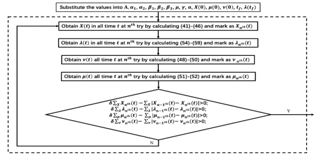
To satisfy (53)–(59), a Forward–Backward Sweep (FBS) method is applied. The flow diagram of the method is illustrated in Figure6. First, the supposed values of model parameters are given. Then, by applying the finite difference method, the numerical solutions of the state variables are calculated in order and adjoint variables in reversed order. Furthermore, the values of controls are obtained at the same time. Finally, if and only if the difference between the two iterations is less than an error valueδmultiplied
by the iteration value at the current moment, then the optimality conditions stated in Theorem5are considered to be satisfied. Here, we setδ=0.001. It is worth noting that,
when the system has low computational complexity, the FBS method can achieve better convergence of the adjoint variables. However, with the increasing complexity of the system, the method has difficulty achieving convergence, and it needs to update, which is also one of the directions of our future work.
Figure 6.Flow diagram of Forward–Backward Sweep (FBS) method.
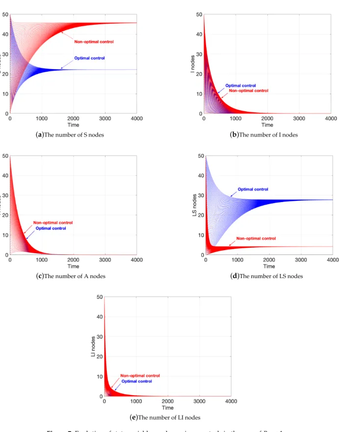
Figure7shows the comparison of evolution of state variables under optimal control and non-optimal control. Here, the blue lines represent the evolution under optimal control and the red lines represent the evolution under non-optimal control. In Figure7a, we set up 100 datasets, in which cases of the optimal control and the non-optimal control are equally divided. In the sets under optimal control, we assume that the sum of the initial number of nodesSandIof the networks is 50. For example, when the initial number ofSnodes is 24, the initial number ofInodes is 26. Figure7a shows the comparison of the number ofSnodes in the two cases. Figure7a shows that the number ofSnodes under optimal control reach the equilibrium point more quickly, and the number is less than that under non-optimal control. Furthermore, the number ofSnodes under optimal control is lower than that under non-optimal control when the number stay steady.
The data in Figure7b follow those in Figure7a. In the case of optimal control, as the number ofSnodes decreases, the number ofInodes decreases more rapidly, as shown in Figure7b. In other words, malware is eliminated faster under optimal control.
In the setting of the data of the two cases in Figure7c, we assume that it containsA andInodes at the beginning, and the sum is 50. As illustrated in Figure7c, the difference in the number ofAnodes is not evident in the two cases, which indicates the removal action never stops.
In Figure7d, we assume that it contains onlyLSandLInodes at the beginning, and their sum is 50. As illustrated in Figure7d, the reason for the decrease in the number ofS nodes is that WRSNs choose to stop charging theLSnodes, which leads to an increase to the number ofLSnodes.
The data setting in Figure7e follows that in Figure7d. Similarly, the difference in the number ofLInodes is not significant in the two cases, as shown in Figure7e, which indicates the software attacks never stop.
Therefore, although the spread of malicious programs can be suppressed under the optimal control, the performance of the system is sacrificed, that is, the existence of more low-energy sensor nodes leads to problems in network operation.
(a)The number of S nodes (b)The number of I nodes
(c)The number of A nodes (d)The number of LS nodes
(e)The number of LI nodes
Figure 7.Evolution of state variables under various controls in the case ofR0<1. 4.5. Variation of State Variables when R0>1
In this subsection, the situation underR0>1 is discussed. Comparing with Section4.4,
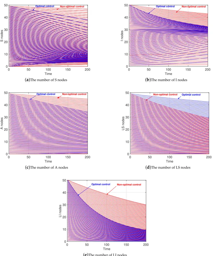
if the value ofTis too high, the adjoint variables do not converge finally under the FBS method, so we set the terminal time of the game to 200, i.e.,T=200. Meanwhile, the data setting is the same as in Section4.5.
Figure8shows the comparison of the changes in the number of the state variables in the same two cases stated in Section4.4. Similar to the statement in Section4.4, the number ofSnodes under optimal control always shows a faster decline, as shown in Figure8a. In contrast, the number ofSnodes with non-optimal control does not change much from time 0 to 200. Therefore, in the case ofR0 >1, WRSNs can restrain the growth ofInodes by
reducing the number ofSnodes.
0 50 100 150 200 Time 0 10 20 30 40 50 S nodes
Optimal control Non-optimal control
(a)The number of S nodes
0 50 100 150 200 Time 0 10 20 30 40 50 I nodes
Optimal control Non-optimal control
(b)The number of I nodes
0 50 100 150 200 Time 0 10 20 30 40 50 A nodes
Optimal control Non-optimal control
(c)The number of A nodes
0 50 100 150 200 Time 0 10 20 30 40 50 LS nodes
Non-optimal control Optimal control
(d)The number of LS nodes
0 50 100 150 200 Time 0 10 20 30 40 50 LI nodes
Optimal control Non-optimal control
(e)The number of LI nodes
Compared with the case without optimal control, moreLSnodes stay in the LS state at this time instead of returning to theS state, as shown in Figure8d. For the case of non-optimal control, the number ofLSnodes decreases rapidly sinceLSnodes constantly send charging requests and get fully charged. For the optimal control,LSnodes choose to stop charging in order to reduce the growth rate ofSnodes’ number.
As illustrated in Figure8b,c,e, with the effective reduction of the number ofSnodes, the numbers ofInodes,Anodes, andLInodes all show a significant decrease, compared with the situation under non-optimal control.
In the case ofR0 > 1, for malware, to make the cost as large as possible, the three
means controlled by malware maintain the maximum degree of control; for WRSNs, in addition to removing malware in the maximum efforts, it also stops charging theLSnodes to further deter more vulnerable nodes from being attacked.
4.6. Influence of Parameters under Optimal Controls
As in Section4.3, the influence of parameters on malware is developed here. It is easy to know from Section4.4that, whenR0<1, malware is completely eliminated eventually.
Therefore, we only consider the caseR0>1. At the same time, to maintain the continuity
with Section4.3, supposeT=200.
Figure9shows the influence of the parameters on the number ofInodes, and the range of the parameters is consistent with Section4.3. It is worth mentioning that, at this time, since the time setting is much smaller than that in Section4.3, the number ofInodes is larger. Comparing with Figure5in Section4.3, it is not difficult to find that, under optimal control, the influence of parameters on the propagation of malware is very similar to that under non-optimal control. Similarly, the conclusion is similar to Section4.3, and is not repeated here.
In the optimal dynamic game, the three control methods of malware, namelyASI(t), AID(t), andALI I(t), are always present and undiminished. As WRSNs, it stops charging the LS nodes while exerting greatest effort to activate the anti-malware program. Therefore, in the game process, the overall architecture of SIALS model is not affected. In other words, stopping charging has little effect on the model. Meanwhile, this phenomenon also reveals that the influence of reduced charging rate on the spread of malware mainly occurs in the state transition of sensor nodes fromLIstate to Istate.
0 1 10 0.01 I nodes 20 1 0.05 2 30 0.005 0.01 0.0001
(a)Variation trend under variousα1andα2
0 1 10 0.01 I nodes 20 1 0.05 3 30 0.005 0.01 0.0001
(b)Variation trend under variousα1andβ3
5 1 10 0.01 15 I nodes 20 0.05 2 25 0.005 0.01 0.0001
(c)Variation trend under variousγandα2
10 1 15 0.01 I nodes 20 0.05 3 25 0.005 0.01 0.0001
(d)Variation trend under variousγandβ3
10 0.01 15 0.01 I nodes 20 3 0.005 2 25 0.005 0.0001 0.0001
(e)Variation trend under variousβ3andα2
0 1 10 0.01 I nodes 20 0.05 1 30 0.005 0.01 0.0001
(f)Variation trend under variousγandα1
Figure 9.Change of infection in optimal controls under various parameters when t = 200. 5. Conclusions
In this paper, we use epidemiology to propose a dynamic model, namely SIALS, describing the propagation of malware in WRSNs. In this model, not only the remaining energy of the sensor nodes is revealed, but also the description of the recovered process is enriched by introducing the anti-malware (A) state. Meanwhile, through the stability analysis of the model, we proved the local and global stability of disease-free equilibrium point and the epidemic equilibrium point. Furthermore, based on the confrontational nature of malware and WRSNs, this paper proposes a five-tuple attack–defense game model. Specifically, after introducing the overall cost, by adopting the Pontryagin Maximum Principle, this paper introduces the dynamic optimal strategies for malware and WRSNs. We verified the validity of the theories through simulations in the form of three-dimensional figures and analyzed the influence of the parameters on the propagation of malware. Then, the evolution of the number of state variables based on optimal control in the two cases of R0 < 1 and R0 > 1 was also simulated and analyzed. Meanwhile, the influence of
parameters on infection under optimal control was analyzed.
Simulation results show that the malware can be eliminated by adjusting the trans-mission rate, but it needs to be reduced to a certain threshold. Activating anti-malicious program is the most effective and direct way to suppress the spread of malware. Adjusting the charging rate can also suppress the spread of malware effectively, but, again, it needs to be below a certain threshold. In the dynamic game between malware and WRSNs, WRSNs
effectively reduce the number of malware by refusing to charge. In particular, in the case ofR0<1, malware goes extinct more quickly. In the case ofR0>1, the spread of malware
is suppressed obviously compared with the case with non-optimal control.
With the continuous development of the wireless power transfer and the intelligent mobile vehicles, the potential security risk of mobile charger cannot be ignored. In our future work, in view of the integrating of various devices, both the homogenous and het-erogenous cases will be taken into consideration, and, if the ability permits, the stochastic modeling and the advanced mathematical theories will be applied. Consequently, we hope our works can give some inspirations to interested researchers.
Author Contributions:Conceptualization, G.L. and B.P.; methodology, G.L., B.P. and X.Z.; software, B.P.; validation, G.L., B.P. and X.Z.; formal analysis, B.P.; investigation, G.L. and B.P.; writing—original draft preparation, B.P.; and writing—review and editing, G.L., B.P. and X.Z. All authors have read and agreed to the published version of the manuscript.
Funding:The National Natural Science Foundation of China (61403089) and the 2020 Department of Education of Guangdong Province Innovative and Strong School Project (Natural Sciences) - Young Innovators Project (Natural Sciences) under Grant 2020KQNCX054.
Conflicts of Interest:The authors declare no conflict of interest References
1. Xie, H.M.; Yan, Z.; Yan, Z.; Atiquzzaman, M. Data Collection for Security Measurement in Wireless Sensor Networks: A Survey.
IEEE Internet Things J.2020,6, 2205–2224.
2. Han, G.J.; Jiang, J.F.; Zhang, C.Y.; Duong, T.Q.; Guizani, M.; Karagiannidis, G.K. A Survey on Mobile Anchor Node Assisted Localization in Wireless Sensor Networks.IEEE Commun. Surv. Tutor.2016,18, 2220–2243.
3. Butun, I.; Osterberg, P.; Song, H.B. Security of the Internet of Things: Vulnerabilities, Attacks, and Countermeasures. IEEE Commun. Surv. Tutor.2020,22, 616–644.
4. Rashid, B.; Rehmani, M.H. Applications of wireless sensor networks for urban areas: A survey.J. Netw. Comput. Appl.2016,60, 192–219.
5. Yetgin, H.; Cheung, K.T.K.; El-Hajjar, M.; Hanzo, L. A Survey of Network Lifetime Maximization Techniques in Wireless Sensor Networks.IEEE Commun. Surv. Tutor.2017,19, 828–854.
6. Panatik, K.Z.; Kamardin, K.; Shariff, S.A.; Yuhaniz, S.S.; Ahmad, N.A.; Yusop, O.M.; Ismail, S. Energy Harvesting in Wireless Sensor Networks: A Survey. In Proceedings of the 2016 IEEE 3rd international symposium on Telecommunication Technologies (ISTT), Kuala Lumpur, Malaysia, 28–30 November 2016.
7. Shu, Y.C.; Yousefi, H.; Cheng, P.; Chen, J.M.; Gu, Y.; He, T.; Shin, K.G. Near-Optimal Velocity Control for Mobile Charging in Wireless Rechargeable Sensor Networks.IEEE. Trans. Mob. Comput.2016,15, 1699–1713.
8. Wu, P.F.; Xiao, F.; Sha, C.; Huang, H.P.; Sun, L.J. Trajectory Optimization for UAVs’ Efficient Charging in Wireless Rechargeable Sensor Networks.IEEE Trans. Veh. Technol.2020,69, 4207–4220.
9. Mo, L.; Kritikakou, A.; He, S.B. Energy-Aware Multiple Mobile Chargers Coordination for Wireless Rechargeable Sensor Networks.
IEEE Internet Things J.2019,6, 8202–8214.
10. Lin, C.; Shang, Z.; Du, W.; Ren, J.K.; Wang, L.; Wu, G.W. CoDoC: A Novel Attack for Wireless Rechargeable Sensor Networks through Denial of Charge. In Proceedings of the IEEE INFOCOM 2019-IEEE Conference on Computer Communications, Paris, France, 29 April–2 May 2019.
11. Lin, C.; Zhou, J.Z.; Guo, C.Y.; Song, H.B.; Wu, G.W.; Mohammad, S.O. TSCA: A temporal-spatial real-time charging scheduling algorithm for on-demand architecture in wireless rechargeable sensor networks.IEEE. Trans. Mob. Comput.2018,17, 211–224. 12. Nguyen, A.N.; Vo, V.N.; So-ln, C.; Ha, D.B.; Sanguanpong, S.; Baig, Z.A. On Secure Wireless Sensor Networks With Cooperative
Energy Harvesting Relaying.IEEE Access2019,7, 139212–139225.
13. Jung, J.; Kang, M.; Yoon, I.; Noh, D.K. Adaptive Forward Error Correction Scheme to Improve Data Reliability in Solar-powered Wireless Sensor Networks. In Proceedings of the 2016 International Conference on Information Science and Security (ICISS), Pattaya, Thailand, 19–22 December 2016.
14. Vo, V.N.; Nguyen, T.G.; So-ln, C.; Ha, D.B. Secrecy Performance Analysis of Energy Harvesting Wireless Sensor Networks with a Friendly Jammer.IEEE Access2017,5, 25196–25206.
15. Shafie, A.E.I.; Niyato, D.; Al-Dhahir, N. Security of Rechargeable Energy-Harvesting Transmitters in Wireless Networks.IEEE Wirel. Commun. Lett.2016,5, 384–387.
16. Bhushan, B.; Sahoo, G. E2SR2: An acknowledgement-based mobile sink routing protocol with rechargeable sensors for wireless sensor networks.Wirel. Netw.2019,25, 2697–2721.
17. Lim, S.; Huie, L. Hop-by-Hop Cooperative Detection of Selective Forwarding Attacks in Energy Harvesting Wireless Sensor Networks. In Proceedings of the 2015 International Conference on Computing, Networking and Communications, Anaheim, CA, USA, 16–19 February 2015.
18. Kommuru, K.J.S.R.; Kadari, K.K.Y.; Alluri, B.K.S.P.K.R. A novel approach to balance the trade-off between security and energy consumption in WSN. In Proceedings of the 2018 2nd International Conference on Micro-Electronics and Telecommunication Engineering, Ghaziabad, India, 20–21 September 2018.
19. Mauro, A.D.; Fafoutis, X.; Dragoni, N. Adaptive Security in ODMAC for Multihop Energy Harvesting Wireless Sensor Networks.
Int. J. Distrib. Sens. Netw.2015,11, 760302.
20. Hu, X.; Huang, K.Z.; Chen, Y.J.; Xu, X.M.; Liang, X.H. Secrecy Analysis of UL Transmission for SWIPT in WSNs with Densely Clustered Eavesdroppers. In Proceedings of the 2017 9th International Conference on Wireless Communications and Signal Processing (WCSP 2017), Nanjing, China, 11–13 October 2017.
21. Bouachir, O.; Mnaouer, A.B.; Touati, F.; Crescini, D. Opportunistic Routing and Data Dissemination Protocol for Energy Harvesting Wireless Sensor Networks. In Proceedings of the 2016 8th IFIP International Conference on New Technologies, Mobility and Security (NTMS 2016), Larnaca, Cyprus, 21–23 November 2016.
22. Huang, S.Y.; Chen, F.D.; Chen, L.J. Global dynamics of a network-based SIQRS epidemic model with demographics and vaccination.Commun. Nonlinear Sci. Numer. Simul.2017,43, 296–310.
23. Srivastava, P.K.; Pandey, S.P.; Gupta, N.; Singh, S.P.; Ojha, R.P. Modeling and Analysis of Antimalware Effect on Wireless Sensor Network. In Proceedings of the 2019 IEEE 4th International Conference on Computer and Communication Systems (ICCCS), Singapore, 23–25 February 2019.
24. Zhu, L.H.; Guan, G. Dynamical analysis of a rumor spreading model with self-discrimination and time delay in complex networks.
Physics A2019,533, 121953.
25. Liu, G.Y.; Peng, B.H.; Zhong, X.J. A Novel Epidemic Model for Wireless Rechargeable Sensor Network Security.Sensors2020,21, 123. doi:10.3390/s21010123
26. Hosseini, S.; Azgomi, M.A. The dynamics of an SEIRS-QV malware propagation model in heterogeneous networks.Physics A
2018,512, 803–817.
27. Ojha, R.P.; Srivastava, P.K.; Sanyal, G.; Gupta, N. Improved Model for the Stability Analysis of Wireless Sensor Network Against Malware Attacks.Wirel. Pers. Commun.2020, 1–24. doi:10.1007/s11277-020-07809-x
28. Huang, D.W.; Yang, L.X.; Yang, X.F.; Wu, Y.B.; Tang, Y.Y. Towards understanding the effectiveness of patch injection.Physics A
2019,526, 120956.
29. Zhu, L.H.; Zhou, M.T.; Zhang, Z.D. Dynamical Analysis and Control Strategies of Rumor Spreading Models in Both Homogeneous and Heterogeneous Networks.J. Nonlinear Sci.2020,30, 2545–2576.
30. Guillén, J.D.H.; del Rey, A.M. A mathematical model for malware spread on WSNs with population dynamics.Physics A2020,
545, 123609.
31. Shen, S.G.; Zhou, H.P.; Feng, S.; Liu, J.H.; Zhang, H.; Cao, Q.Y. An Epidemiology-Based Model for Disclosing Dynamics of Malware Propagation in Heterogeneous and Mobile WSNs.IEEE Access2020,8, 43876–43887.
32. Eshghi, S.; Khouzani, M.H.R.; Sarkar, S. Optimal Patching in Clustered Malware Epidemics.IEEE-ACM Trans. Netw.2016,24, 283–298.
33. Khouzani, M.H.R.; Sarkar, S.; Altman, E. Optimal Dissemination of Security Patches in Mobile Wireless Networks.IEEE Trans. Inf. Theory2012,58, 4714–4732.
34. Zhang, L.T.; Xu, J. Differential Security Game in Heterogeneous Device-to-Device Offloading Network under Epidemic Risks.
IEEE Trans. Netw. Sci. Eng.2020,7, 1852–1861.
35. Al-Tous, H.; Barhumi, I. Differential Game for Resource Allocation in Energy Harvesting Sensor Networks. In Proceedings of the 2018 IEEE International Conference on Communications (ICC), Kansas City, MO, USA, 20–24 May 2018.
36. Huang, Y.H.; Zhu, Q.Y. A Differential Game Approach to Decentralized Virus-Resistant Weight Adaptation Policy over Complex Networks.IEEE Trans. Control Netw. Syst.2020,7, 944–955.
37. Sun, Y.; Li, Y.B.; Chen, X.H.; Li, J. Optimal defense strategy model based on differential game in edge computing.J. Intell. Fuzzy Syst.2020,39, 1449–1459.
38. Shen, S.G.; Li, H.J.; Han, R.S.; Vasilakos, A.V.; Wang, Y.H.; Cao, Q.Y. Differential Game-Based Strategies for Preventing Malware Propagation in Wireless Sensor Networks.IEEE Trans. Inf. Forensics Secur.2014,9, 1962–1973.
39. Hu, J.H.; Qian, Q.; Fang, A.; Fang, S.Z.; Xie, Y. Optimal Data Transmission Strategy for Healthcare-Based Wireless Sensor Networks: A Stochastic Differential Game Approach.Wirel. Pers. Commun.2016,89, 1295–1313.
40. Sarkar, S.; Khouzani, M.H.R.; Kar, K. Optimal Routing and Scheduling in Multihop Wireless Renewable Energy Networks.IEEE Trans. Autom. Control2013,58, 1792–1798.
41. Liu, G.Y.; Peng, B.H.; Zhong, X.J.; Cheng, L.F.; Li, Z.F. Attack-Defense Game between Malicious Programs and Energy-Harvesting Wireless Sensor Networks Based on Epidemic Modeling.Complexity2020,2020, 3680518.
42. Van den Diressche, P.; Watmough, J. Further notes on the basic reproduction number. InMathematical Epidemiology; Brauer, F., van den Driessche, P., Wu, J., Eds.; Springer: Berlin, Germany, 2008; pp. 159–178.
44. Lasalle, J.P.The Stability of Dynamical Systems; SIAM: Philadelphia, PA, USA, 1976.
45. Merkin, D.R.Introduction to the Theory of the Stability; Springer: New York, NY, USA, 2012; Volume 24.
46. Robinson, R.C.An Introduction to Dynamical Systems: Continous and Discrete; Pearson Education; Prentice Hall: Upper Saddle River, NJ, USA, 2004.