A Mixed Noise Removal Method Based on Total Variation

A Mixed Noise Removal Method Based on Total Variation

Dang N.H. Thanh

Tula State University; 92 Lenin Ave., Tula, Russian Federation Hue College of Industry, 70 Nguyen Hue st., Hue, Vietnam E-mail: [email protected]

Dvoenko Sergey D.

Tula State University; 92 Lenin Ave., Tula, Russian Federation E-mail: [email protected]

Dinh Viet Sang

Hanoi University of Science and Technology; 1 Dai Co Viet st., Hanoi, Vietnam E-mail: [email protected]

Keywords: total variation, ROF model, gaussian noise, poisson noise, image processing, biomedical image, euler-lagrange equation

Received: March 24, 2016

Due to the technology limits, digital images always include some defects, such as noise. Noise reduces image quality and affects the result of image processing. While in most cases, noise has Gaussian distri-bution, in biomedical images, noise is usually a combination of Poisson and Gaussian noises. This com-bination is naturally considered as a superposition of Gaussian noise over Poisson noise. In this paper, we propose a method to remove such a type of mixed noise based on a novel approach: we consider the superposition of noises like a linear combination. We use the idea of the total variation of an image in-tensity (brightness) function to remove this combination of noises.

Povzetek: Članek predlaga izvirno kombinacijo Gaussovega in Poissonovega filtra za filtriranje šuma v slikah.

1

Introduction

Image denoising has attracted a lot of attention in recent years. In order to suppress noise effectively, we need to know its type. There are many types of noises, for exam-ple, Gaussian (digital images), Poisson (X-Ray images), Speckle (ultra sonograms) noises and so on.

One of the most famous effective methods is the to-tal variation model [2-4, 10, 12, 17, 18, 22, 26]. The first person who suggested it to solve the denoising problem is Rudin [17]. He used the total variation as a universal tool in image processing. His denoising model is well-known as the ROF model [3, 17]. The ROF model is tar-geted to efficiently remove Gaussian noise only.

This model is often used to remove not only Gaussi-an noise, but also other types of noise. For example, the ROF model suppresses Poisson noise not so effectively. Le T. [9] proposed another model, well-known as the modified ROF model to remove Poisson noise only.

Gaussian and Poisson noises both are widespread in real situations, but their combination is important too, for example, in electronic microscopy images [7, 8]. In these images, both types of noises are combined as a superpo-sition. In physical process, Poisson noise usually is added first, before Gaussian noise. Luisier F. with co-authors proposed the theoretically strong PURE-LET method [11] (Poisson-Gaussian unbiased risk estimate – linear expansion of thresholds) to remove this type of combina-tion of noises.

However, such kind of noises usually can be consid-ered as dependent on the image acquisition systems. At the same time, in many papers devoted to the image de-noising problem the idea of Poisson-Gaussian noise combination is considered, even though such is not the case.

From other side, many noise reduction approaches have been developed, particularly, wavelet-based trans-forms, etc. It needs to draw attention, noise reduction approaches that have been developed based on wavelet transform are only for Gaussian or Poisson noise.

In order to remove mixed noise, let us assume that the superposition of noises can be equivalent to some unknown linear combination of them.

We can combine ROF and modified ROF models to suppress the linear combination of noises. The obtained model is supposed to remove the mixed noise better than ROF or modified ROF models separately. Additionally, it is simpler than PURE-LET, because we try to find only the proportion between Poisson and Gaussian noises in the mixed noise.

compared results with Wiener [1] and median [23] filters, and with Beltrami method [29]. Our method gives better results for Gaussian and Poisson noises separately, and for the combination of noises too. Hence, in this paper, we do not compare our approach with these methods.

In order to compare image quality after restoration, we use criteria PSNR (Peak Signal-to-Noise Ratio), MSE (Mean Square Error), SSIM (Structure SIMilarity) [24, 25]. The PSNR criterion is the most important, because it is always used to evaluate images and signals quality.

In this paper, we try to represent and discuss only the case limited by the greyscale artificial and real images with artificial noise. According to it, we can use only criteria above based on the full-reference image quality evaluation approach.

In the case of greyscale real images with unknown noises, we need to use the no-reference approach to eval-uate the quality of denoising. In general, it is complicated theoretical problem to develop a criterion for it.

Our investigation based on BRISQUE criterion [13] (Blind/Referenceless Image Spatial QUality Evaluator) in this case was discussed in paper [20].

2

Combined denoising model

Let in 2

R space a bounded domain 2

R

  be given. Let functions u x y( , )R and v x y( , )R, respectively, be ideal (without noise) and observed (noisy) imag-es,( , )x y . For smooth function u, its total variation

can be defined by V u_T[ ] | u dxdy|



 

_

, where

( _x, _y)

u u u

  is a gradient, ux   u/ x, uy  u/ y,

2 2

| u| uxuy . In this paper, we consider that the

func-tion u always has limited total variation V uT[ ] .

According to [2, 3, 17, 18], an image smoothness is characterized by the total variation of an image intensity function. The total variation of the noisy image is always greater than the total variation of the corresponding smooth image. In order to solve the problem

[ ] min

T

V u  , we need to use the following condition 2

(v u dxdy) const



 



.

Hence, we obtain the ROF model to remove Gaussi-an noise in the image [17, 18]:

2

arg min | | ( )

2

u

u u dxdy v u dxdy

 

 

 _    _











,

where



0 is Lagrange multiplier. This is a solution of the unconstrained optimization problem.

In order to remove Poisson noise, Le T. built another model based on ROF model [9] as the optimization prob-lem V uT[ ]min with the following constraint

ln( ( | ))p v u dxdy (u vln( ))u dxdy const

 

  





.

This model resulted in the following unconstrained optimization problem

*

arg min | | ( ln( ))

u

u u dxdy u v u dxdy

 

 

     









,

where



0 is a coefficient of regularization. This is the known modified ROF model to remove Poisson noise.

In order to build a model for removing the mixed Poisson-Gaussian noise, we also solve the same optimi-zation problem V uT[ ]min, but with a different

con-straint as follows.

This constraint is very similar to constraints above. We consider, the noise variance is unchangeable (Pois-son noise is not changed and Gaussian noise only de-pends on noise variance):

ln( ( | ))p v u dxdy const 





, (1)

where p v u( | ) is a conditional probability of the real image v with the ideal image u given.

The probability density function of Gaussian noise is 2

1 2

( )

( | ) exp / ( 2 )

2

v u p v u  _  _







 

,

and the probability distribution of Poisson noise is

2( | ) exp( ) / !

v

p v u  u u v .

We have to notice that intensity functions of images

u and v are integer (for example, for 8-bits greyscale image the range of intensity is from 0 to 255).

In order to combine Gaussian and Poisson noises, we consider the following linear combination

1 1 2 2

ln( ( | ))p v u ln(p v u( | )) ln(p v u( | )),

10

 , ₂ 0,  ₁ ₂1.

According to (1), we obtain the denoising problem as a constrained optimization problem

*

2 1

2 2

arg min | |

( ) ( ln( )) ,

2

u

u u dxdy

v u u v u dxdy





  



  

 _    _ 

  







  



where  is a constant value. We transform this problem into unconstrained optimization problem by using La-grange functional

2 1

2

( , ) | | ( )

2

L u u dxdy v u dxdy

 



   _  















2 (u vln( ))u dxdy





  









to find the solution as * *

,

( , ) arg min ( , )

u

u  L u



  (2)

where



0 is Lagrange multiplier.

If ₁0 and    ₂ , we obtain the modified ROF model to remove Poisson noise. If ₂ 0 and

2 1 /



3

Discrete denoising model

The problem (2) can be solved by using Lagrange multi-pliers method [5, 16, 28].

We use Euler-Lagrange equation [28]. Let a function

( , )

f x y be defined in a limited domain 2

R

  and be second-order continuously differentiated by x and y,

where ( , )x y . Let F x y f f( , , , _x,f_y) be a convex functional, where fx  f / x, fy   f / y. Then the

solution of the following optimization problem ( , , , _x, _y) min

F x y f f f dxdy







satisfies the following Euler-Lagrange equation

( , , , , ) ( , , , , )

x

f x y f x y

F x y f f f F x y f f f x



 



( , , , , ) 0

y

f x y

F x y f f f y





 ,

where F_f  F/f , / x

f x

F  F f , /

y

f y

F  F f .

We use the above result to solve the obtained model. Then the solution of the problem (2) satisfies the follow-ing Euler-Lagrange equation

1

2

2( ) (1 )

v v u

u

     

2 2 2 2 0,

y x

x y x y

u u

x _{u u} y _{u u}

     _{ }  _{ }      _{  }  _{  }





(3)

where 1 /. We rewrite (3) in the form

1

2

2( ) (1 )

v v u u    



_



2 2

2 2 3/ 2

2

0

( )

xx y x y xy x yy x y

u u u u u u u

u u    



, (4) 2 2 xx u u x    _, 2 2 yy u u y    , xy yx u u u u

x y y x

 

      _{ } _{ }

      _.

In order to obtain the discrete form of the model (4), we add an artificial time parameter and consider the function

( , , )

uu x y t in the following diffusion equation

1

2

2( ) (1 )

t

u v

u v u

t u            2 2

2 2 3/ 2

2

( )

xx y x y xy x yy x y

u u u u u u u

u u

 





.

(5)

Then the discrete form of the equation (5) is

1 1

2( )

k k k

i j i j i j i j

u  u   v u 









2(1 )

i j k i j k i j v u    _ 





, (6) 2

2 2 3/ 2

( )( ( ))

(( ( )) ( ( )) )

k k

xx ij y ij k

i j k k

x ij y ij

u u u u       



2

2 2 3/ 2

2 ( ) ( ) ( ) ( ( )) ( )

(( ( )) ( ( )) )

k k k k k

x ij y ij xy ij x ij yy ij

k k

x ij y ij

u u u u u

u u           , 1, 1, ( ) 2 k k i j i j k x ij u u u x       ,

, 1 , 1 ( )

2

k k i j i j k y ij u u u y       , 1, 1, 2 2 ( ) ( )

k k k

i j ij i j k

xx ij

u u u

u

x

   

 

 ,

, 1 , 1

2 2 ( )

( )

k k k

i j ij i j k

yy ij

u u u

u

y

   

 

 ,

1, 1 1, 1 1, 1 1, 1 ( )

4

k k k k

i j i j i j i j k

xy ij

u u u u

u

x y

          

 

  ,

1 1 2 2

0 1; 1, , ; 0 1; , 1 , ;

k k k k k k k k

j j N j N j i i i N i N

u u u  u u u u  u

1 2

1,..., ; 1,..., ;

i N j N

0,1,..., ; 1; 0 1

k K    x y   , where K is enough great number, K500.

4

Optimal model parameters

In practice, parameters    ₁, ₂, , in procedure (6) are

usually unknown. We have to change   ₁, ₂, into

1, 2,

k k k

   to evaluate them on every iteration step k.

4.1

Optimal parameters λ

1

and λ

2

Let ( , )u be a solution of problem (2). Then we obtain the following condition L u( , ) /  u 0. This condition

give us optimal ₁ and ₂:

1

2

(1 )

1

( ) (1 )

v dxdy u

v v u dxdy dxdy

u        







 

, ₂  1 ₁.

The discrete form for k0,1,...,K is

1 2 1 2 1 1 1 2 1 1 (1 )

( 1 )

N N ij k i j ij k

k N N

ij ij ij k

i j ij

v u

v u v

u         





 

, ₂k  1 ₁k.

4.2

Optimal parameter μ

In order to find the optimal



, we multiply (3) by

(v u ) and integrate by parts over domain . Finally, we obtain the formula to find the optimal

2 2 1 2 2 2 2 2 2 ( ) ( ( ) )

( x y x x y y)

x y

v u

v u dxdy

u u v u v

u u dxdy

u u           





 _   .

The discrete form is

1 2 1 2 2 2 1 2 2 1 1 1 1 ( ) ( ( ) ) k N N k

ij ij k k

ij ij k

i j ij

2 2

( ( )) ( ( ))

k k k

ij  x uij  y uij 



2 2

( ) ( ) ( ) ( )

( ( )) ( ( ))

k k

x ij x ij y ij y ij

k k

x ij y ij

u v u v

u u         , 1, 1, ( ) 2 k k i j i j k x ij u u u x       ,

, 1 , 1 ( )

2

k k i j i j k y ij u u u y       , 1, 1, ( ) 2 k k i j i j k x ij v v v v x       ,

, 1 , 1 ( )

2

k k i j i j k y ij v v v y       ,

1 1 2 2

0 1; 1, , ; 0 1; , 1 , ;

k k k k k k k k

j j N j N j i i i N i N

u u u _ u u u u _ u

1 1 2 2

0j 1j; N 1,j N j; i0 i1; i N, 1 i N, ;

v v v _ v v v v _ v

1 2

1,..., ; 1,..., ;

i N j N k0,1,..., ;K    x y 1.

4.3

Optimal parameter σ

The parameter  is calculated at the first step of the iteration process. We use the method of Immerker [6]:

1 2

1 1

1 2

/ 2

| * |

6( 2)( 2)

N N ij i j

u

N N  

 

 





 ,

with the mask

1 2 1 2 4 2 1 2 1



 



 

   

  for convolution operator *,

1, 1 33 , 1 32 1, 1 31 1, 23 *

ij i j i j i j i j

u  u_{ } u _ u_{ } u_  

22 1, 21 1, 1 13 , 1 12 1, 1 11

ij i j i j i j i j

u  u_  u_{ } u _ u_{ } ,

1 2

1,..., ; 1,..., ;

i N j N 0

ij

u  , if i0, or j0, or iN₁1, or jN₂1.

4.4

Initial solution

In the iteration procedure (6), the result depends on ini-tial parameters 0 0 0

1, 2,

   . If 0 0 0 1, 2,

   are given first, then its unsuitable values define not so good solution u_ij

and later, not so good evaluation of a probability distri-bution parameters. If   ₁0, ₂0, 0 are randomized, the re-sult is unacceptable too, because of the additional noise added in the image.

Of course, initial values of 0 0 0 1, 2,

   need to be closed to required values. We evaluate 0 0 0

1, 2,

   as av-erage values of neighbour pixels of the image, for exam-ple, by the method of Immerker.

5

Image quality evaluation

In order to evaluate the image quality after denoising, we use criteria PSNR, MSE and SSIM [24, 25]:

1 2 2 MSE 1 1 1 2 1

Q ( )

N N

ij ij i j

v u

N N  





 , 2 PSNR MSE Q 10lg Q L    _{ }  , 1 2

SSIM 2 2 2 2

1 2

(2 )(2 )

Q

( )( )

uv u v

u v C C

u v C C

          , where 1 2 1 1 1 2

1 N N

ij i j

u u

N N  





,

1 2

1 1 1 2

1 N N

ij i j

v v

N N  





. 1 2 2 2 1 1 1 2 1 ( ) 1 N N u ij i j u u

N N  

  



 , 1 2 2 2 1 1 1 2 1 ( ) 1 N N v ij i j v v

N N  

  



 , 1 2 1 1 1 2 1 ( )( ) 1 N N

uv ij ij

i j

u u v v

N N  

  





 ,

2 2

1 ( 1 ) , 2 ( 2 ) ; 1 1; 2 1

C  K L C  K L K  K  .

For example, 6

1 2 10

K K   , L is an image intensi-ty with L255 for 8-bits greyscale image.

The greater the value of Q_PSNR, the better the image

quality. If the value of Q_PSNR belongs to the interval

from 20 to 25, then the image quality is acceptable, for example, for wireless transmission [21].

The Q_MSE is a mean squared error and is used to evaluate the difference between two images. The lower the value of Q_MSE, the better the result of restoration.

The value of Q_MSE directly related to the value of Q_PSNR.

The value of Q_SSIM is used to evaluate an image quality by comparing the similarity of two images. This value is between -1 and 1. The greater the value of

SSIM

Q , the better the image quality.

6

Experiments and discussion

In this paper, we consider cases as in [19] and additional-ly the superposition of noises. The image size is changed from 300x300 pixels to 256x256 pixels specified in PURE-LET method [11]. We process the artificial image with artificial noise and the real image with artificial noise. The artificial image is noise-free and we need to add noise with high intensity (the image to be very noisy) to reduce its quality. Therefore, we specify 0.6 for pro-portion of Gaussian noisy image and 0.4 for propro-portion of Poisson noisy image. The real image (captured by a digital device) already includes some noise. We specify 0.5 for proportion of Gaussian noisy image and 0.5 for proportion of Poisson noisy image too.

We need to point the attention in the case of Gaussi-an noise our method sometimes cGaussi-an be better thGaussi-an ROF, because the method to evaluate the variance of Gaussian noise can be better than one included in the original ROF model in many cases. In the case of superposition of noises, our method sometimes can be better than PURE-LET, because parameters of our method are usually more optimal than in original model too.

6.1

Artificial image with artificial noise

We use artificial image with artificial mixed noise for the first test. The image includes eight bars (Fig. 1a). Other images (Fig. 1b-j) show noisy and denoised images and zoomed out part of them.

Artificial noise is generated by linear combination, and by superposition of Poisson and Gaussian noises.

For both cases, we consider Poisson noise first. Its

at every pixel ( , )i j , i1,...,N₁, j1,...,N₂. Poisson

noise variance is an average value ₂11.7939. If the grey value of a pixel after adding of Poisson noise is out of the interval from 0 to 255, it needs to be reset to

(2)

i j i j

v u . For this image, there are no pixels out of this interval. Next, we consider the variance of Gaussian noise is four times greater than the variance of Poisson

noise ₁4₂47.1757.

For the linear combination of noises, we denote the intensity function of Gaussian noisy image as (1)

v . As above, values of (1)

v need to be between 0 and 255. If the grey value of a pixel after adding of Gaussian noise is out of the interval from 0 to 255, it needs to be reset to

(1)

i j i j

v u . In this case, there are 1075 pixels out of this

a) b)

c) d)

e) f)

g) h)

i) j)

Figure 1: Denoising of the artificial image: a)-b) original image, c)-d) noisy image with linear combi-nation of noises, e)-f) denoised image (c), g)-h) noisy image with superposition of noises, i)-j) denoised image (g).

a) b)

c) d)

e) f)

g) h)

i) j)

interval (1.64%).

The final noisy image (linear combination of noises in Fig. 1c) is created with proportion 0.6 for Gaussian noisy image (1)

v and proportion 0.4 for Poisson noisy image (2)

v : (1) (2)

0.6 0.4

v v  v .

Then we define proportion for linear combination as



 



1/ 2  0.6 47.1757 / 0.4 11.7939  6 / 1

  .

Coeffi-cients of linear combination are defined as

1 = 6/7 = 0.8571, 2 = 1/7 = 0.1429.

Values of QPSNR, QMSE, and QSSIM of the noisy im-age (linear combination of noises) are, respectively, 19.4291, 741.5963, and 0.1073.

In the case of the image with superposition of noises, we add Gaussian noise over Poisson noisy image. The intensity function of this Gaussian noisy image is (1)

v too. As above, the grey values of v(1) need to be between 0 and 255. If the grey value of a pixel after adding of

Gaussian noise is out of the interval from 0 to 255, it needs to be reset to v_{i j}(1) v_{i j}(2).

There are 1220 pixels out of this interval (1.86%). The noisy image (superposition of noises, Fig. 1g) is also Gaussian noisy image vv(1). In this case, we don’t know 1 and 2, therefore we use the algorithm with au-tomatically defined parameters.

Values of QPSNR, QMSE, and QSSIM of the noisy im-age are, respectively, 14.9211, 2093.9827, and 0.0439.

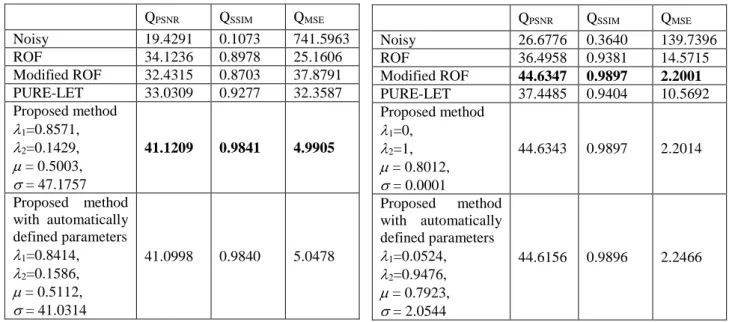
Tables 1 – 4 show results for linear combination of noises, Gaussian noise, Poisson noise, and superposition of noises for the artificial image.

6.2

Real image with artificial noise

The artificial noise is generated by linear combination and superposition of Poisson and Gaussian noises.

For both cases, we consider Poisson noise first. Pois-son noise variance is an average value ₂ 9.0882. If the grey value of a pixel after adding of Poisson noise is out of the interval from 0 to 255, it needs to be reset to

QPSNR QSSIM QMSE

Noisy 19.4291 0.1073 741.5963

ROF 34.1236 0.8978 25.1606

Modified ROF 32.4315 0.8703 37.8791

PURE-LET 33.0309 0.9277 32.3587

Proposed method

1=0.8571,

2=0.1429,

 = 0.5003,

 = 47.1757

41.1209 0.9841 4.9905

Proposed method with automatically defined parameters

1=0.8414,

2=0.1586,

 = 0.5112,

 = 41.0314

41.0998 0.9840 5.0478

Table 1: Quality of noise removing for the artificial image with linear combination of noises.

QPSNR QSSIM QMSE

Noisy 15.1406 0.0457 1990.8

ROF 31.4797 0.8364 21.2502

Modified ROF 28.4591 0.7871 27.5694

PURE-LET 28.9451 0.7986 25.9883

Proposed method

1=1, 2=0,

 = 0.3033,

 = 47.1757

35.8011 0.9598 16.8122

Proposed method with automatically defined parameters

1=0.9715,

2=0.0285,

 = 0.3021,

 = 46.0314

35.7589 0.9596 17.2658

Table 2: Quality of noise removing for the artificial image with Gaussian noise.

QPSNR QSSIM QMSE

Noisy 26.6776 0.3640 139.7396

ROF 36.4958 0.9381 14.5715

Modified ROF 44.6347 0.9897 2.2001

PURE-LET 37.4485 0.9404 10.5692

Proposed method

1=0,

2=1,

 = 0.8012,

 = 0.0001

44.6343 0.9897 2.2014

Proposed method with automatically defined parameters

1=0.0524,

2=0.9476,

 = 0.7923,

 = 2.0544

44.6156 0.9896 2.2466

Table 3: Quality of noise removing for the artificial image with Poisson noise.

QPSNR QSSIM QMSE

Noisy 14.9211 0.0439 2093.983

ROF 31.2913 0.8346 48.3008

Modified ROF 30.5471 0.8232 56.5601

PURE-LET 33.9889 0.9298 25.9534

Proposed method with automatically defined parameters

1=0.8014,

2=0.1986,

 = 0.4812,

 = 40.0314

37.3366 0.9677 12.0066

(2)

i j i j

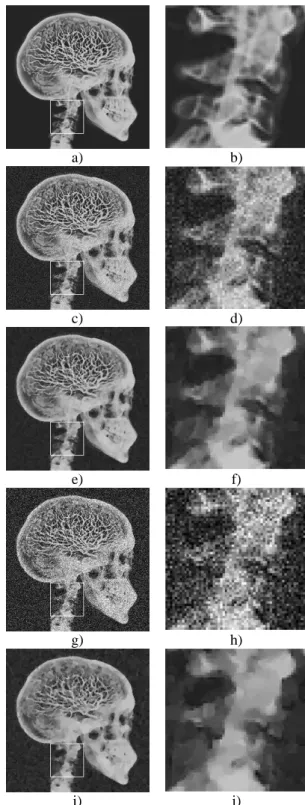
v u . Here there are no pixels out of this interval. For Gaussian noise, we consider the variance of Gaussian noise is four times greater than the variance of Poisson noise ₁4₂36.3529. The real image is a human skull [14] (Fig. 2a). Others (Fig. 2b-j) show noisy and denoised images and zoomed out part of them.

For the case of linear combination of noises, we de-note the intensity function of Gaussian noisy image as

(1)

v . As above, the grey values of intensity function (1) v also need to be between 0 and 255. If the grey value of a pixel after adding of Gaussian noise is out of the interval from 0 to 255, it needs to be reset to vi j(1)ui j. In this

case, there are 5355 pixels out of this interval (8.17%). The final image (linear combination of noises, Fig. 2c) is created with proportion 0.5 for Gaussian noisy image (1)

v and proportion 0.5 for Poisson noisy image (2)

v : (1) (2)

0.5 0.5

v v  v . The proportion for linear

combina-tion is:  ₁/ ₂(0.5 36.3529) / (0.5 9.0882  )4 1/ . Hence, coefficients of linear combination are defined as 1 = 4/5 =0.8, 2 = 1/5 = 0.2. Values of QPSNR, QMSE, and QSSIM of final noisy image are, respectively, 23.6878, 278.1619, and 0.5390.

For superposition of noises, we add Gaussian noise over Poisson noisy image. We denote the intensity func-tion of Gaussian noisy image as v(1). As above, grey val-ues of (1)

v need to be between 0 and 255. If the grey val-ue after adding of Gaussian noise is out of the interval from 0 to 255, it needs to be reset to v_{i j}(1) v_{i j}(2). In this case, there are 5621 pixels out of this interval (8.58%). The final noisy image (superposition of noises, Fig. 2g) is also the Gaussian noisy image vv(1).

In this case, we don’t know 1 and 2, therefore we use the algorithm to find them. Values of QPSNR, QMSE, and QSSIM of the final noisy image (superposition) are, respectively, 17.8071, 1077.3831, and 0.3242.

Tables 5 – 8 show results for linear combination of noises, Gaussian noise, Poisson noise, and superposition of noises for the real image.

QPSNR QSSIM QMSE

Noisy 23.6878 0.5390 278.1619

ROF 27.3974 0.8295 118.3975

Modified ROF 25.5644 0.7513 197.5403

PURE-LET 25.7781 0.8105 191.0341

Proposed method

1=0.8, 2=0.2,

 = 0.0524,

 = 36.3529

27.6641 0.8331 110.9451

Proposed method with automatically defined parameters

1=0.7804,

2=0.2196,

 = 0.0512,

 = 34.2311

27.6039 0.8325 112.8984

Table 5: Quality of noise removing for the real im-age with linear combination of noises.

QPSNR QSSIM QMSE

Noisy 18.0693 0.3337 1014.3

ROF 24.0246 0.7299 257.4095

Modified ROF 23.2511 0.7019 311.8742

PURE-LET 23.8712 0.7989 265.6153

Proposed method

1=1, 2=0,

 = 0.0956,

 = 36.3529

24.2011 0.8029 242.5101

Proposed method with automatically defined parameters

1=0.9538,

2=0.0462,

 = 0.0902,

 = 35.0633

24.1882 0.8028 247.8894

Table 6: Quality of noise removing for the real im-age with Gaussian noise.

QPSNR QSSIM QMSE

Noisy 28.4991 0.7625 91.8683

ROF 31.0567 0.9457 50.9818

Modified ROF 31.1992 0.9022 48.9375

PURE-LET 30.8955 0.8678 53.1066

Proposed method

1=0, 2=1,

 = 0.0541,

 = 0.0001

31.1334 0.8986 49.7922

Proposed method with automatically defined parameters

1=0.0491,

2=0.9509,

 = 0.0567,

 = 4.2012

31.1316 0.8986 50.1094

Table 7: Quality of noise removing for the real image with Poisson noise.

QPSNR QSSIM QMSE

Noisy 17.8077 0.3242 1077.383

ROF 23.1936 0.7062 311.6856

Modified ROF 23.0413 0.7033 319.3831

PURE-LET 23.6278 0.7072 282.0349

Proposed method with automatically defined parameters

1=0.7704,

2=0.2296,

 = 0.1102,

 = 36.3412

23.7292 0.7094 275.5229

6.3

About of initial solution

In order to create the initial image, we use the convolu-tion operator. The table 9 shows the dependency of re-stored result for the initial image, where:

(a) Initial parameters 0 0

1 0, 2 1, 1

   ;

(b) Initial parameters 0 0

1  2 0.5, 1

   ;

(c) Initial solution 0

u is given as a randomized matrix; (d) Initial solution 0

u  v is given as an average val-ue of neighbour pixels by the convolution operator with the mask  



1 / 9



of the size 3x3.

Table 9 shows the best result of denoising is (d) by criteria PSNR and MSE.

The result (c) by SSIM looks different in contract to ones in Tables 1-8. It illustrates incorrectness of a ran-domized initial solution (accidental and not stable, if a probability distribution is unknown).

Next, we have to notice that the non-optimal result (a) has been used in experiments for Table 5. It appears to be enough for the good result with automatically de-fined model parameters.

(a) (b) (c) (d)

1 0.7804 0.8094 0.8733 0.8032

2 0.2196 0.1906 0.1267 0.1968

 0.0512 0.0573 0.0653 0.0565

 34.2311

QPSNR 27.6039 27.2214 26.5611 27.6523 QMSE 112.8984 120.4355 132.0264 107.5431 QSSIM 0.8325 0.8317 0.8395 0.8392 Table 9: Dependency of denoising on initial solution.

At last, the variant (b) initially looks better than (a) for kind of better assumption of ₁0 ₂00.5 to process the real image. Nevertheless, our assumption about 1

is very far from the good one, and evidently the limit of the number of steps K500 is insufficient in this case.

As a result, the variant (d) is the best idea for initial solution.

7

Conclusion

In this paper, we proposed a novel method that can effec-tively remove the mixed Poisson-Gaussian noise. Fur-thermore, our proposed method can be also used to re-move Gaussian or Poisson noise separately. This method is based on the variational approach.

The denoising result strongly depends on values of coefficients of linear combination ₁ and ₂. These val-ues can be set manually or can be defined automatically. When processing real images, we can use the proposed method with automatically defined parameters.

Although our method concentrates on removing the linear combination of noise, but it also efficiently re-moves the superposition of noises. In this case, we con-sider the superposition of noises is equivalent to some linear combination of them with coefficients found in iteration process.

In this paper we show that our simple model “feels” well the wide range of proportion of two types of noises. As a result, it appears to be the good basis for removing superposition of such noises.

It is evident, the iteration process (6) used here is in-sufficiently effective in comparing with other possible computational schemes. In this paper, we try to compare our approach to image denoising with PURE-LET meth-od only in possible reduction of our mmeth-odel complexity, not in others.

We would like to express our great thanks to devel-opers of PURE-LET method for kindly granted us the original executable module of it.

8

Acknowledgements

This work is partially supported by Russian Foundation for Basic Research, under grants 13-07-00529, 14-07-00964, 15-07-02228, 16-07-01039, and by Ministry of Education and Training, Vietnam, under grant number B2015–01–90.

References

[1] Abe C., Shimamura T. Iterative Edge-Preserving adaptive Wiener filter for image denoising. ICCEE, 2012, Vol. 4, No. 4, P. 503-506.

[2] Chan T.F., Shen J. Image processing and analysis:

Variational, PDE, Wavelet, and stochastic methods.

SIAM, 2005.

[3] Chen K. Introduction to variational image pro-cessing models and application. International

jour-nal of computer mathematics, 2013, Vol. 90, No.1,

P.1-8.

[4] Getreuer P. Rudin-Osher-Fatemi total variation

denoising using split Bregman. IPOL 2012:

http://www.ipol.im/pub/art/2012/g-tvd/.

[5] Gill P.E., Murray W. Numerical methods for

con-strained optimization. Academic Press Inc., 1974.

[6] Immerker J. Fast noise variance estimation.

Com-puter vision and image understanding, 1996, Vol.

64, No.2, P. 300-302.

[7] Jezierska A. An EM approach for Poisson-Gaussian noise modelling. EUSIPCO 19th_{, 2011,}

Vol. 62, Is. 1, P. 13-30.

[8] Jezierska A. Poisson-Gaussian noise parameter estimation in fluorescence microscopy imaging.

IEEE International Symposium on Biomedical

Im-aging 9th_{, 2012, P. 1663-1666.}

[9] Le T., Chartrand R., Asaki T.J. A variational ap-proach to reconstructing images corrupted by Pois-son noise. Journal of mathematical imaging and vi-sion, 2007, Vol. 27, Is. 3, P. 257-263.

[10] Li F., Shen C., Pi L. A new diffusion-based varia-tional model for image denoising and segmentation.

Journal mathematical imaging and vision, 2006,

Vol. 26, Is. 1-2, P. 115-125.

[11] Luisier F., Blu T., Unser M. Image denoising in mixed Poisson-Gaussian noise. IEEE transaction

on Image processing, 2011, Vol. 20, No. 3, P.

[12] Lysaker M., Tai X. Iterative image restoration com-bining total variation minimization and a second-order functional. International journal of computer

vision, 2006, Vol. 66, P. 5-18.

[13] Mittal A., Moorthy A.K., and Bovik A.C. No refer-ence image quality assessment in the spatial do-main, IEEE Trans. Image Processing 21 (12), 4695–4708 (2012).

[14] Nick V. Getty images: http://well.blogs.nytimes .com/2009/09/16/what-sort-of-exercise-can-make-you-smarter/.

[15] Rankovic N., Tuba M. Improved adaptive median filter for denoising ultrasound images. Advances in

computer science, 2012, P.169-174.

[16] Rubinov A., Yang X. Applied Optimization: La-grange-type functions in constrained non-convex

optimization. Springer, 2003.

[17] Rudin L.I., Osher S., Fatemi E. Nonlinear total var-iation based noise removal algorithms. Physica D., 1992, Vol. 60, P. 259-268.

[18] Scherzer O. Variational methods in Imaging. Springer, 2009.

[19] Thanh N. H. Dang, Dvoenko Sergey D., Dinh Viet Sang. A Denoising Method Based on Total

Varia-tion. Proc.of 6th _{Intern. Symposium on Information}

and Communication Technology (SoICT-2015). P. 223-230. ACM, NY, USA.

[20] Thanh D.N.H., Dvoenko S.D. A method of total variation to remove the mixed Poisson-Gaussian noise. Pattern Recognition and Image Analysis, 26 (2), 285-293 (2016).

DOI: 10.1134/S1054661816020231.

[21] Thomos N., Boulgouris N.V., Strintzis M.G. Opti-mized Transmission of JPEG2000 streams over Wireless channels. IEEE transactions on image

processing, 2006, Vol. 15, No.1, P .54-67.

[22] Tran M.P., Peteri R., Bergounioux M. Denoising 3D medical images using a second order variational model and wavelet shrinkage. Image analysis and

recognition, 2012, Vol. 7325, P. 138-145.

[23] Wang C., Li T. An improved adaptive median filter for Image denoising. ICCEE, 2012, Vol. 53, No. 2.64, P. 393-398.

[24] Wang Z. Image quality assessment: From error vis-ibility to structural similarity. IEEE transaction on

Image processing, Vol. 13, No. 4, P. 600-612.

2004.

[25] Wang Z., Bovik A.C. Modern image quality

as-sessment. Morgan & Claypool Publisher, 2004.

[26] Xu J., Feng X., Hao Y. A coupled variational model for image denoising using a duality strategy and split Bregman. Multidimensional systems and

sig-nal processing, 2014, Vol. 25, P. 83-94.

[27] Zhu Y. Noise reduction with low dose CT data based on a modified ROF model. Optics express, 2012, Vol. 20, No. 16, P. 17987-18004.

[28] Zeidler E. Nonlinear functional analysis and its applications: Variational methods and optimiza-tion. Springer, 1985.

[29] Zosso D., Bustin A. A Primal-Dual Projected Gra-dient Algorithm for Efficient Beltrami