SIMULATING, RECONSTRUCTING, AND ROUTING METROPOLITAN-SCALE TRAFFIC
David Wilkie
A dissertation submitted to the faculty of the University of North Carolina at Chapel Hill in partial fulfillment of the requirements for the degree of Doctor of Philosophy in the
Department of Computer Science.
Chapel Hill 2015
Approved by:
Ming C. Lin
Ron Alterovitz
Anselmo Lastra
Dinesh Manocha
c ○2015 David Wilkie
ABSTRACT
David Wilkie: Simulating, Reconstructing, and Routing Metropolitan-Scale Traffic. (Under the direction of Ming C. Lin.)
Few phenomena are more ubiquitous than traffic, and few are more significant
economi-cally, socially, or environmentally. The vast, world-spanning road network enables the daily
commutes of billions of people and makes us mobile in a way our ancestors would have
en-vied. And yet, few systems perform so poorly so often. Gridlock and traffic jams cost 2.9
billion gallons of wasted fuel and costs over 121 billion dollars every year in the U.S. alone.
One promising approach to improving the reliability and efficiency of traffic systems is to
fully incorporate computational techniques into the system, transforming the traffic systems
of today into cyber-physical systems. However, creating a truly cyber-physical traffic system
will require overcoming many substantial challenges. The state of traffic at any given time is
unknown for the majority of the road network. The dynamics of traffic are complex, noisy,
and dependent on drivers’ decisions. The domain of the system, the real-world road network,
has no suitable representation for high-detail simulation. And there is no known solution for
improving the efficiency and reliability of the system.
In this dissertation, I propose techniques that combine simulation and data to solve these
challenges and enable large-scale traffic state estimation, simulation, and route planning.
First, to create and represent road networks, I propose an efficient method for enhancing
high-detail, real-time traffic simulation, interactive visualization, traffic state estimation, and
vehicle routing. The resulting representation provides important road features for traffic
simulations, including ramps, highways, overpasses, merge zones, and intersections with
arbitrary states.
Second, to estimate and communicate traffic conditions, I propose a fast technique to
reconstruct traffic flows from in-road sensor measurements or user-specified control points
for interactive 3D visualization and communication. My algorithm estimates the full state
of the traffic flow from sparse sensor measurements using a statistical inference method and
a continuum traffic model. This estimated state then drives an agent-based traffic simulator
to produce a 3D animation of traffic that statistically matches the sensed traffic conditions.
Third, to improve real-world traffic system efficiency, I propose a novel approach that
takes advantage of mobile devices, such as cellular phones or embedded systems in cars, to
form an interactive, participatory network of vehicles that plan their travel routes based on
the current, sensed traffic conditions and the future, projected traffic conditions, which are
estimated from the routes planned by all the participants. The premise of this approach is
that a route, or plan, for a vehicle is also a prediction of where the car will travel. If routes
are planned for a sizable percentage of the vehicles using the road network, an estimate for
the overall traffic pattern is attainable. If fewer cars are being coordinated, their impact
on the traffic conditions can be combined with sensor-based estimations. Taking planned
routes into account as predictions allows the entire traffic route planning system to better
For each of these challenges, my work is motivated by the idea of fully integrating traffic
simulation, as a model for the complex dynamics of real world traffic, with emerging data
ACKNOWLEDGMENTS
I want to thank the members of GAMMA Lab, especially Jason Sewall, Jur van den Berg,
Sujeong Kim, Abhinav Golas, Ravish Mehra, my committee members, and my advisor, Ming
TABLE OF CONTENTS
LIST OF TABLES. . . xiv
LIST OF FIGURES. . . xv
1 Introduction. . . 1
1.1 Traffic Systems . . . 2
1.1.1 Road Networks. . . 2
1.1.1.1 Directed Graph . . . 3
1.1.1.2 Polyline Road Networks . . . 3
1.1.1.3 Lanes, Geometry, and Intersections . . . 4
1.1.2 Traffic state . . . 4
1.1.3 Boundary Conditions . . . 5
1.1.4 Dynamics . . . 5
1.2 Sensor Data . . . 6
1.2.1 Loop Detectors. . . 7
1.2.2 Traffic Cameras . . . 7
1.2.3 GPS-Enabled Mobile Devices . . . 8
1.3 Thesis Statement . . . 8
1.4 Main Results . . . 9
1.4.2 Detailed Traffic Reconstruction.. . . 10
1.4.3 Self-Aware Route Planning.. . . 11
1.4.4 Mobile System for Participatory Routing. . . 12
1.5 Organization . . . 12
2 Road Networks . . . 14
2.1 Introduction. . . 14
2.2 Related Work. . . 16
2.2.1 GIS Data, Tools, and Software Systems . . . 17
2.2.2 Geometric Representation . . . 18
2.3 Preliminaries . . . 19
2.3.1 Simulation Requirements . . . 19
2.3.1.1 Discrete Simulation. . . 20
2.3.2 Continuum simulation . . . 21
2.3.3 System Overview. . . 22
2.3.4 GIS Data Filtering . . . 23
2.4 A Lane-Centric Graph Representation. . . 24
2.4.1 Roads. . . 25
2.4.1.1 Road Split . . . 25
2.4.1.2 Road Join. . . 25
2.4.1.3 Proof of Road Creation. . . 26
2.4.2 Lanes . . . 28
2.4.3 Intersections. . . 29
2.4.3.2 Ramp Intersections. . . 31
2.5 Overpasses and Underpasses . . . 32
2.5.1 Intersection Points. . . 33
2.5.2 Road Height Levels. . . 33
2.6 Results. . . 35
2.7 Summary. . . 36
3 State Estimation. . . 37
3.1 Introduction. . . 37
3.2 Related Work. . . 40
3.3 Approach. . . 43
3.3.1 Preliminaries . . . 43
3.3.2 State Estimation . . . 45
3.3.2.1 Overview. . . 45
3.3.2.2 Flow Reconstruction. . . 46
3.3.2.3 Ensemble Initialization . . . 49
3.3.2.4 Motion Model. . . 49
3.3.2.5 Observation Model . . . 52
3.3.2.6 Tuning and Noise . . . 52
3.3.3 Detailed Reconstruction . . . 52
3.3.3.1 Overview. . . 52
3.3.3.2 Vehicle Instantiation . . . 53
3.3.3.3 Particle Advection. . . 54
3.3.4 Merging. . . 55
3.4 Results. . . 58
3.4.1 Data . . . 58
3.4.2 Metric . . . 59
3.4.3 Experiments. . . 59
3.4.3.1 Error in Mean Flow . . . 59
3.4.4 Implementation Details. . . 60
3.4.5 Performance Analysis. . . 60
3.4.6 Comparison with Related Work. . . 61
3.5 Summary. . . 63
3.5.1 Limitations. . . 64
3.5.2 Future Work . . . 64
4 Self-Aware Route Planning. . . 65
4.1 Introduction. . . 65
4.2 Related Work. . . 67
4.3 Approach. . . 68
4.3.1 Route Planning. . . 70
4.3.1.1 Density and Travel Time . . . 70
4.3.1.2 Cost Function. . . 71
4.3.1.3 Planning Algorithm . . . 72
4.3.2 Maintaining Density Functions. . . 73
4.3.2.1 Blending Historical and System Data . . . 74
4.4 Empirical Results. . . 76
4.4.1 Traffic Simulation . . . 77
4.4.2 Avoiding Congestion on a Single Path. . . 78
4.4.3 Comparison with Shortest Path Planner. . . 78
4.4.4 Comparison with Stochastic Planner Using Historical Data . . . 80
4.4.5 Effect of Adoption Rate . . . 81
4.5 Summary. . . 83
5 Participatory Routing: Real-World Road Networks and Prototype System. . . 84
5.1 Introduction. . . 84
5.2 Related Work. . . 86
5.3 Prototype System . . . 88
5.4 Algorithms . . . 90
5.4.1 Mathematical Framework. . . 90
5.4.2 Participatory Route Planning. . . 92
5.4.2.1 Traffic Jams. . . 92
5.4.2.2 Intersection Delay . . . 94
5.5 Experiments. . . 96
5.5.1 Travel Time Prediction . . . 96
5.5.2 Baselines. . . 98
5.5.2.1 Shortest-Path Router (SP). . . 98
5.5.2.2 Sensor-Data Router (SD). . . 98
5.5.3 Scenarios. . . 98
5.5.3.2 Sioux Falls . . . 100
5.5.4 Results. . . 102
5.5.4.1 Manhattan. . . 102
5.5.4.2 Sioux Falls . . . 104
5.5.5 System Performance. . . 107
5.5.6 Discussion. . . 108
5.6 Summary. . . 108
6 Conclusion . . . 110
6.1 Summary of Results . . . 110
6.2 Limitations. . . 111
6.3 Future Work. . . 112
A Appendix. . . 115
A.1 Road Network Geometry. . . 115
A.2 Arc Formulation. . . 117
A.3 Fitting arc roads to polylines. . . 119
A.4 Offset polylines. . . 119
A.5 Discrete approximations of arc roads . . . 120
A.5.1 Polylines . . . 120
A.5.2 Triangle meshes . . . 121
A.6 Road mesh geometry . . . 122
LIST OF TABLES
5.1 Performance speedup of my approach over the Shortest Path (SP) and Sensor-Data (SD) baseline route planning. my method achieves upto a maximum speedup of 18.35 over SP baseline in congested traffic
LIST OF FIGURES
1.1 A road network created by my method with simulated traffic.. . . 9
1.2 An animation of a reconstructed traffic state.. . . 10
1.3 On the left, traffic from shortest path routes. On the right, traffic
from my routing system.. . . 11
1.4 A use case diagram for my routing system. . . 12
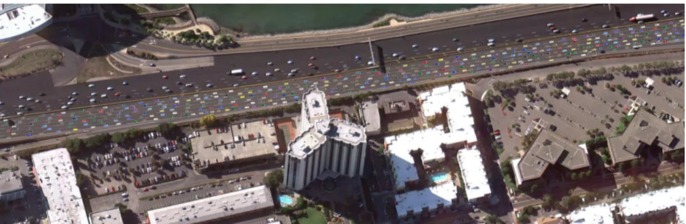
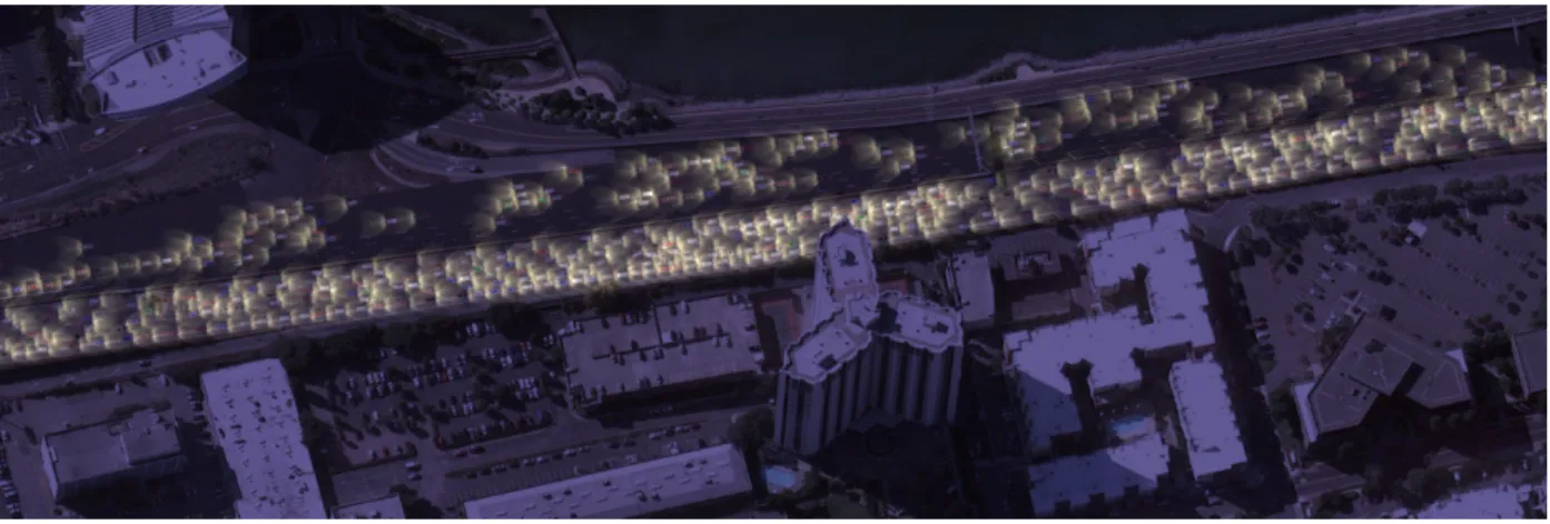
2.1 A road network generated directly from GIS data by my method. The road network has been overlaid on top of a satellite image. Note that the cars on the road network are animated using a traffic simulator
running on my road network representation.. . . 15
2.2 Geometry for a simple road network created by CityEngine®[Prodecural Inc., 2011] is shown in (a). In (b), I show the geometry created by our method for a similar road network. Note that only the lanes in the intersections that currently have a
green light are shown.. . . 18
2.3 A simple intersection with three roads. For each road, I calculate an offset, o, based on each of its neighbors. Here, I see the calculation of the offset for the road A with respect to B. To calculate the offset, first the position of a circle tangent to A and B is calculated with a radius such that a car turning fromA toB will have a turning radius of r. The offset is then the length on A from the intersection to the
projection of the center of the circle ontoA.. . . 30
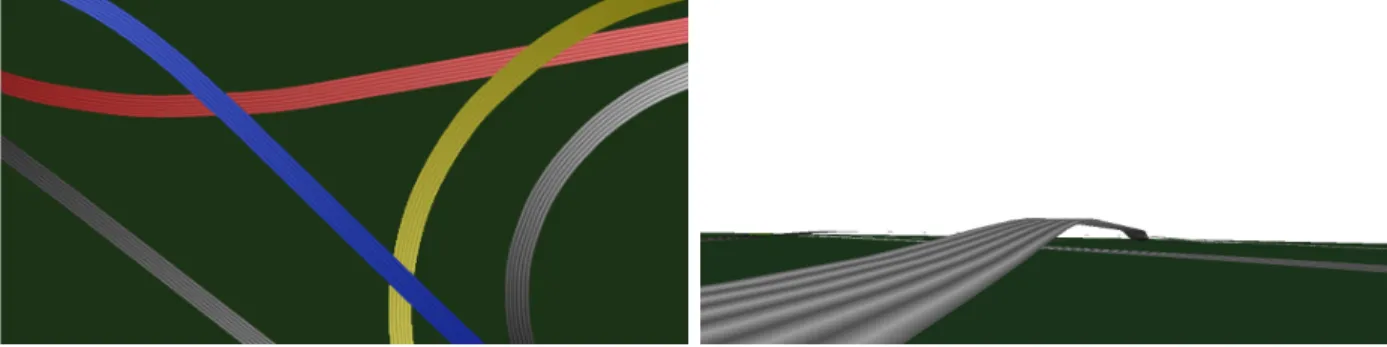
2.4 A highway interchange with overpasses generated by our method. Top: An overhead view of a highway interchange with overpasses. The highways are colored to show the arrangement computed by our method. Bottom: A view of the blue highway, which is given the
greatest height.. . . 32
2.5 A collection of road networks, all generated by our method. The
traffic in these figures was simulated using the technique of [Sewall et al., 2010a] 34
2.6 A series of images showing ramps smoothly connected to a highway,
3.1 The divided highway is populated with traffic using my flow recon-struction method. Individual virtual cars are animated, and the dy-namic state corresponds to the real-world traffic conditions observed
by sensors. . . 37
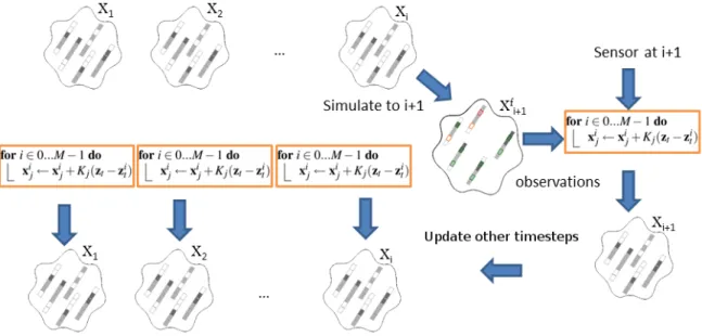
3.2 A schematic view of the approach. . . 44
3.3 The initialization of the smoothing process.. . . 46
3.4 An ensemble member is simulated forward in time, then corrected given the sensor measurement. Finally, previous ensembles are
up-dated to account for the new sensor reading. . . 47
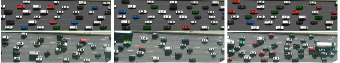
3.5 In this figure, there are three comparisons between the reconstruction and video footage from 5:17, 5:21, 5:25 (Minutes two, six, and ten for the 5:15 data set). In the first image, we see our method over estimates the density in at least two of the lanes in this area. In the next two images, congested traffic is both reconstructed and found in the source data. We can see lane-specific features of the traffic are reconstructed: in all cases, the HOV lane shows a much lower density (and has a higher velocity) than the other lanes. (It should be noted
that the camera placement for the reconstruction images is only approximate.) 57
3.6 The lane-mean density and velocity for a lane of highway traffic. The greenline is the ground truth, theredline is the state estimate, and
the blue line is the agent-based simulation. . . 63
4.1 A schematic picture illustrating the idea of our approach. A road network is shown with edge costs. (a) If a route from s to g is re-quested, the optimal path is computed (shown with thick arrows). If the car follows this route, the densities and hence the edge costs along its path increases (in this case with 1). In (b), the network with the updated edge costs are shown. If a same query (s, g) comes in from a subsequent car, it takes a different route (shown with thick arrows) to avoid the increased traffic densities. Note that this schematic picture
does not illustrate the stochastic and time-varying aspects of our approach. . . 69
4.2 The fundamental diagram relating traffic density to travel speed. . . 70
4.3 The modified A* algorithm to compute an optimal route with respect to the exponential cost metric between start node s and goal node g when traffic is commenced at time t0. When planning has finished, the optimal route is inferred by following the backpointers from the
4.4 We highlight the performance of our algorithm compared with routing cars along a single path. The flow of cars quickly leads to congestion and long travel times for the single path. Our approach distributes
the cars and settles to a constant travel time.. . . 77
4.5 This figure shows the speedup factor that our method achieves over a shortest path planner for a series of cars. Each car has a random
start and goal position. . . 79
4.6 This figure shows the speedup factor (up to 20 for the 100-car mean) that our method achieves over a stochastic planner using only histor-ical data for a series of cars, indexed from 0 to 2500. Each car has a
random start and goal position.. . . 80
4.7 The 100-car mean speedup of our method over the simple planner for
varying adoption percentages.. . . 82
5.1 A System Architecture of Participatory Route Planning: The mobile clients send route queries to the central planner, which takes the updated traffic and routing information from participants and live traffic sensor information to plan a new route for each
par-ticipating client in the network. . . 84
5.2 System overview of our client- and server-side model: The client-side component is portrayed in the diagram (with the orange background) and illustrates our mobile app system; the routing query is received from the client, serialized, and sent to the server, which handles the request. The server-side component (shaded in blue back-ground) shows the handling of the routing query and our participatory route planning process. The routing algorithm is ran with respect to the destination request, the stochastic road map is updated, and the
optimal route in term of travel time is sent back to the client. . . 88
5.3 Different screens featured by our Android App (from left to right): (a) the Main Screen, hosting the interactive map display and destination prediction output; (b) the Locations Screen, showing pre-vious destination queries; (c) the Route Confirmation Screen, detail-ing the route to destination; (d) the En Route to Destination Screen, portraying turn-by-turn directions for the user to follow and the
in-teractive map display.. . . 89
5.4 The A* algorithm to compute an optimal route with respect to the cost metric between start nodesand goal nodeg at timet0. τ values
5.5 The mean travel time for the simulated ground truth (red), my method (green), and the self-aware routing algorithm (blue) for the MSMD scenario, described below. My method can closely track the ground-truth travel time, while the self-aware algorithm systemat-ically underestimates the actual travel time due to its inability to
account for intersection delay.. . . 97
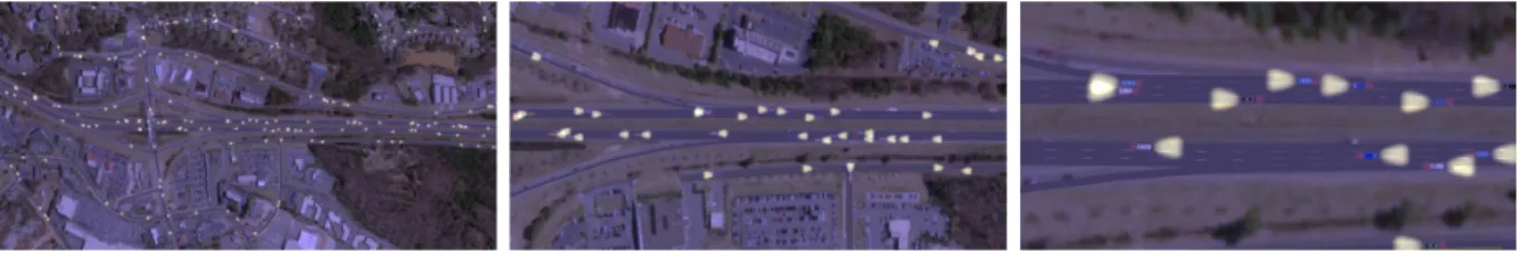
5.6 An example of the MSSD scenario: in which vehicles are spawned at various origin points and drive to a single destination. On the left is the mean velocity field of the fastest-path baseline router, and on the right is the mean velocity field resulting from my method. The destination point was chosen randomly inside the destination re-gion, designated by the red rectangle. The origin points were chosen randomly outside this region with the additional constraint that they be at least 1km away from the destination. The mean velocity is shown as a color ranging from red, 0 m/s, to green, 13 m/s, the speed
limit for most of the roads. . . 99
5.7 This figure shows the origins (blue) and the destinations (red) for the
Sioux Falls morning rush hour commute. . . 101
5.8 MSMD Scenario: These histograms show the performance of my system relative to the SP baseline router for a city-traffic scenario. On the top is shown the time saved by each vehicle by using my system, and on the bottom is shown the speedup of each car achieved by my system. For this example, the mean speedup of my system
over the baseline was 1.48, and the mean time saved was 5.21 minutes.. . . 103
5.9 This figure shows the mean travel times for varying numbers of vehicles using my method, a shortest-path baseline (SP), and a commercial-like system using sensor data (SD). I observe that my method (red) outperformed both the shortest-path baseline (navy)
and the commercial-like system with sensor data (sky blue). . . 105
5.10 Each plot shows the mean velocity field over a ten minute time win-dow, with a color ranging from red, 0 m/s, to green, 13 m/s. The top row is the ground truth; the middle row is the velocity field predicted solely by aggregating the routing requests of participating cars; the
bottom row is the velocity field from using [Wilkie et al., 2011].. . . 106
5.11 This figure shows the number of routes the server can generate in a
period of time.. . . 107
A.2 The quantities defining an arc i corresponding to interior point pi.
The orientation vector oi is coming out of the page. . . 117
A.3 A ‘fattened’ arc road; the original arc road PS as computed above
is drawn in black. The blue lines represent the same shape offset to
either side by an equal distance.. . . 120
CHAPTER 1: INTRODUCTION
Few phenomena are more ubiquitous in the modern world than traffic, and few are more
significant economically and socially. The vast, world-spanning road network enables the
daily commutes of billions of people and makes us mobile in a way our ancestors could not
imagine. And yet, few systems perform so poorly so often. Congestion and gridlock cost
2.9 billion gallons of wasted fuel and over 121 billion dollars every year in the U.S. alone.
[Schrank et al., 2012].
One promising approach to improving the reliability and efficiency of traffic systems
is to fully incorporate computational technology, transforming today’s traffic systems into
cyber-physical systems. However, creating truly cyber-physical traffic systems will require
overcoming many substantial challenges. Currently, the state of traffic at a given time is
unknown for a large majority of the road network, though recent research attempts to patch
together discrete and disparate data sources for a fuller view. The dynamics of the system
are also complex, noisy, and computationally costly to simulate for large networks or large
numbers of vehicles: the system has both continuous aspects, the flow of traffic, and discrete
aspects, such as the cycles of intersections; the dynamics can be approximated with physical
laws, but ultimately emerge from decisions made by drivers. And the domain of the system,
the road network, is complex topologically and geometrically with no widely available
high-detail models.
This dissertation proposes new computational models and approaches that build toward
achieving a cyber-physical traffic system. One component of such a system is traffic
simula-tion, which allows us to efficiently model the complex dynamics of real-world traffic. Traffic
and for creating interactive animations, but I will demonstrate that it can also be a powerful
tool for estimating and communicating the state of traffic to achieve more efficient traffic
flows, especially when combined with newly available data sources.
To make headway on a problem as broad and challenging as this, I have focused my
work on three core challenges. First, for the road network domain, my approach is to
create simulation-enabled representations from GIS road network models, which are now
publicly available in vast databases. This involves constructing formal models atop noisy,
human-authored data and creating 3D geometric representations. Second, to estimate and
communicate traffic conditions, I present a method that filters sensor data, which is discrete
in space and time, to create a continuous estimate of traffic conditions that can be used
to create visualizations or predict traffic patterns. Third, to improve the efficiency of the
traffic system, I present an approach that manages traffic flows via participatory routing, in
which the plans for individual vehicles are aggregated to estimate future traffic conditions.
For each of these challenges, my work is motivated by the idea of fully integrating traffic
simulation, as a model for the complex dynamics of real world traffic, with emerging data
sources, including real-time sensors and public databases.
1.1 Traffic Systems
In this dissertation, I address physical systems that are composed of road networks and
vehicles, which I refer to as a traffic system. These systems can also include various types
of sensing, communication, and computational components. In the following, I discuss the
ways in which we can model these systems for both reasoning and computation.
1.1.1 Road Networks
One component of a traffic system is a road network, which can be modeled at varying
1.1.1.1 Directed Graph
A road network can be represented very simply as a directed graph for which edges, E,
represent segments of roadway, and the vertices, V, represent intersections between roads
and terminus points. Each edge can have attributes such as length, number of lanes, speed
limit, etc.
However, a network such as this would not be suited for any visual analysis or highly
detailed simulation, as the geometric details of the road are lost. It also could not handle
problems that require more geometric information, such as determining which roads
corre-spond to a sequence of global-positioning system (GPS) coordinates.
1.1.1.2 Polyline Road Networks
To address these shortcomings, the road network needs to be embedded in a space,
typically a 2D Cartesian space, which the latitude-longitude points often used to define the
roads can be projected into. In this representation, the vertices, Vi, i.e. intersections, have
coordinates indicating their positions, and each edgee, i.e. each road segment, has additional
vertices, Vg
e , that approximate the geometry of the road. The edges and vertices can have
additional attributes, A, as above.
We will call the above apolyline road network, and it is the most common representation
of road networks. Representations such as this are used for nearly all geographic-information
system (GIS) applications, including for online mapping and vehicle routing, and are
avail-able for many countries in public databases.
This representation also has its shortcomings. For one, lanes are not individually
repre-sented. This limits the level of detail at which simulations can be done and limits the level
of analysis. Second, the polyline (or polygonal chain) geometry can be a source of significant
error – real world cars “cut corners”, following curvilinear paths. This is exacerbated at
extent and can encompass complicated topological relationships. Due to this representation,
inelegant solutions arise, such as modeling complex intersections as multiple vertices in an
attempt to capture their geometric and topological details.
1.1.1.3 Lanes, Geometry, and Intersections
To address these issues, additional details can be added to the representation. First,
individual lanes can be represented as full-fledged objects. These lanes need geometric
representations, which can either be distinct or can reference the geometry of an underlying
road segment. Second, intersections also need a more detailed representation: their geometric
extents and topological relations need to be captured. This includes not only a bounding
geometry but internal lanes that connect the incoming and outgoing lanes. Third, a more
detailed geometric representation can be used, such as a higher number of vertices or curves.
Finally, a model is needed for each intersection that defines the behavior of the intersection,
whether the intersection uses a traffic light logic, stop sign, or some other rules of the road.
1.1.2 Traffic state
The other essential component of the traffic system is the vehicles – all the cars, trucks,
motorcycles, etc. This aspect of the system is time-varying1 and can be represented as either
continuous, i.e. density and velocity fields, or discrete, i.e. individual vehicles. Beyond the
vehicles that are on the roads at a particular time, some representation is needed for the
boundary conditions of the system – the sources and sinks for vehicles.
At any point in time, we can refer to the state of the traffic system, which is the
spec-ification of all the time-varying values, such as how many cars are on the road; how fast
the cars are moving; and how many cars are entering the system. The representation of
the state is dependent on how the dynamics of the traffic system are modeled. There are
two primary approaches. First, every vehicle can be represented. This is the most direct
approach: for every car in the real, there is a virtual car in the model with a known
posi-tion along a lane, a velocity, and perhaps other parameters. This type of representaposi-tion is
referred to asmicroscopicin the literature oragent-basedif the car models encapsulate some
decision making ability. Second, the vehicles can be represented as average quantities over
some spatial discretization; i.e. a lane can be divided into cells, and each of these cells can
contain a density value and a velocity value that represent the average of these statistics in
the real world. This type of representation is called macroscopic.
1.1.3 Boundary Conditions
Real world road networks span whole continents. Working with networks this large is
impractical for most applications, so some region of interest must be specified. In reality,
cars pass into and out of this region, and how this flow is represented depends on the
representation of the system dynamics, but examples include constant density and velocity
values or a rate at which cars are spawned at the boundary points. Internal boundaries,
such as large parking lots, can also be modeled in this manner.
1.1.4 Dynamics
Finally, our model requires a definition for the system dynamics, i.e. how the cars
actually move. Like the state representation, there are two broad categories for these models
– microscopic and macroscopic. For the former, individual vehicles are simulated, typically
by calculating an acceleration from the state of the vehicle and the vehicle ahead of it
along the lane. For the latter, differential equations define the evolution of the density and
velocity fields over time. In either case, the model of the dynamics can be embodied in a
simulation, which, if given initial and boundary conditions, can model the evolution of the
1.2 Sensor Data
Even a perfect model of a traffic system is only useful for real world applications if the
system’s state is known, including the boundary conditions. But this is also a difficult
prob-lem: traffic patterns vary day to day, hour to hour, and minute to minute; the distributions
of origins and destinations are largely unknown; few roads have any sensors; and the sensor
data that exists is difficult to fuse, not widely available, and noisy.
However, two emerging trends offer promise that a much fuller and clearer view of traffic
will be available in the near future. The first of these trends is the networking and aggregation
of existing sensor systems, allowing for a more complete view of the traffic system and real
time updates of traffic conditions. The second trend is the proliferation of mobile devices.
These devices enable traffic applications such as routing by vehicle drivers, and, due to their
networked nature, enable the drivers to report, actively or passively, on the nearby traffic
conditions. Together, these two trends promise accurate and widespread sensing, implying
that we can know the state of traffic at any moment in time. And knowing the state of a
system is the first step toward optimizing it.
There are three principal types of traffic sensors: loop detectors, cameras, and mobile
devices. These sensors can be divided into two categories, stationary sensors, such as the
loop detectors and cameras, andmobile sensors, such as the mobile devices. This distinction
is important as the categories provide different types of data: stationary sensors describe
most or all of the traffic state at a fixed location, i.e. they provide Eulerian measurements,
and mobile sensors report measurements along each vehicle’s trajectory, i.e. they provide
1.2.1 Loop Detectors
The first type of sensor is the loop-detector. A loop detector is an induction loop that
can be used to sense the presence of a vehicle. Double loop-detectors can also be used to
calculate the velocity of the passing vehicle.
Loop detectors are installed permanently on many highways and are often deployed
temporarily on primary and secondary roads to gather survey data on traffic patterns. As
such, loop detectors are currently the most common and widely available form of traffic
sensor.
Loop detectors can record every vehicle that passes, their speeds, and other attributes.
It can break this flow data down by individual lanes. They thus provide a wealth of traffic
data. However, a loop detector only provides data at its location. The next sensor on a
highway may be miles away. Between the detectors, the state of traffic can only be estimated.
Most roads do not have this level of sensing, as permanent loop detectors are placed almost
exclusively on highways.
1.2.2 Traffic Cameras
Another form of traffic sensor is the video camera. Cameras provided a real-time view
of a region of the road network, capturing more context than loop detectors. They can also
be relatively inexpensive.
However, cameras do not directly measure the traffic state. That is, they do not provide
a measure of the vehicles’ velocities or how many vehicles there are. This data can be
obtained from a video, but it requires tracking each car and determining the position of the
camera relative to the vehicles. For these reasons, cameras are not widely used to gather
1.2.3 GPS-Enabled Mobile Devices
The third type of sensor is the mobile device, such as a cell phone or dashboard computer,
that is networked and GPS-enabled. These devices are capable of sending periodic updates
of the position of the vehicle. Some can also send direct velocity measurements, and for those
that cannot the velocity can be estimated using the distance the vehicle traveled through
the road network and the time interval between updates. The strength of this type of sensor
is its potential to be ubiquitous – every driver could carry a device, reporting on traffic
conditions throughout the road network.
However, measurements from devices such as this are not yet widely available to the
public or to researchers. The datasets that are available point to some weaknesses. First, it
is unlikely that a high percentage of cars will regularly use a mobile device that reports on the
traffic conditions: the average user only needs a mobile device when traveling somewhere
unfamiliar; sending updates from a persistently running device requires the device to be
plugged in or it drains the battery; and positional updates clearly have privacy implications.
A consequence of this is that data is currently available only in limited areas, and many of
the available datasets were collected from taxi fleets. Second, as only a small percentage of
vehicles can be expected to report the conditions, the data from these sensors is very sparse
in addition to being noisy. Third, these devices are not capable of sensing the total number
of vehicles on the road. And fourth, mobile sensors move with the vehicles, meaning that a
persistent view of a single area of the road network can be difficult to obtain.
1.3 Thesis Statement
My work focuses on integrating computational models of traffic systems, described above,
with newly available and emerging data sources, including both sensor data and publicly
It is possible to integrate traffic simulation with emerging data sources, including mobile
sensing, sensor networks, and public databases, to enable novel traffic system computations,
including simulating traffic throughout whole cities, reconstructing detailed traffic conditions,
and performing participatory multi-vehicle route planning.
To support this thesis, I present my approach to creating road network models,
es-timating and communicating traffic conditions, and optimizing the overall traffic flow via
participatory routing. Finally, I discuss a prototype implementation of this system.
1.4 Main Results
My main results include the following.
1.4.1 Automatic Road Network Creation.
Figure 1.1: A road network created by my method with simulated traffic.
An immense amount of data exits for road networks in the form of Geographic
Infor-mation System (GIS) databases, but the data in this form is not suitable for simulation.
It lacks geometric details, lanes, relations between lanes at intersections, and contains
hu-man error and noise. In Chapter 2, I propose a method to create metropolitan-scale road
networks suitable for simulation and animation from this publicly available GIS data. The
resulting networks will be suitable for real-time, 3D simulation and animation. The method
presents approaches to formalizing the road network, filtering common noise and errors,
cre-ating intersection geometry, and assigning heights and an ordering to highway overpasses
1.4.2 Detailed Traffic Reconstruction.
Figure 1.2: An animation of a reconstructed traffic state.
The most common traffic sensors currently are loop detectors, which are embedded on
many highways throughout the world. Recently, sensor networks of loop detectors have been
created in same areas, enabling real-time data for many important roads. However, this
data is discrete in time, due to aggregation periods, and space, as sensors can be a mile
or farther apart. In Chapter 3, I propose a method to create traffic reconstructions from
loop detector networks such as this, i.e. the method will estimate the time-varying state of
traffic and create a corresponding simulation. Unlike previous work, my method uses the
state-of-the-art, second-order ARZ traffic model [Aw and Rascle, 2000, Zhang, 2002]. The
resulting simulation will recreate traffic that is qualitatively and quantitatively similar to
1.4.3 Self-Aware Route Planning.
Figure 1.3: On the left, traffic from shortest path routes. On the right, traffic from my
routing system.
Even with the knowledge of the state of the traffic system, it can be a challenge to
optimize the overall performance. One possibility is to route vehicles using the knowledge
you have about traffic conditions, but if a large percentage of vehicles are routed, they
themselves determine the future traffic conditions. In Chapter 4, I propose a method that
can efficiently route thousands of vehicles in a manner that minimizes congestion and travel
time. By utilizing my method for estimating a vehicle’s effect on the traffic density field,
my method allows the route planner to take other vehicles into account without any explicit
coordination. In realistic metropolitan-scale simulations, my method achieves a travel time
1.4.4 Mobile System for Participatory Routing.
Figure 1.4: A use case diagram for my routing system.
Finally I propose an architecture, design, and prototype implementation of a system
that implements the self-aware routing technique. The prototype server can handle 1000
near simultaneous routing requests in under 15 seconds, with an average response time of
under a second. Each route planned is used by the system to update its estimation of the
traffic conditions. The mobile client features a novel use of destination prediction for
ease-of-use and a UI similar to existing navigation systems, with a local map of the road network,
highlighted route, and turn-by-turn directions.
1.5 Organization
The remainder of this dissertation is organized as follows. In Chapter 2, I describe my
approach to creating simulation-capable road networks. In Chapter3, I describe my approach
to creating visualizations of traffic conditions from sensor data. In Chapter 4, I present a
theoretical framework for route planning that considers the effect on traffic of the previously
planned routes. In Chapter 5, I expand this method to account for real world conditions
traffic system efficiency. Finally in Chapter6, I present some concluding remarks and discuss
CHAPTER 2: ROAD NETWORKS
2.1 Introduction
Simulation is an important tool for addressing the challenges of traffic system state
estimation, optimization, and visualization. However, traffic simulations take place on a
complex domain, the road network. The acquisition and representation of this domain
present numerous challenges: the domain must match the real-world for the simulation to be
useful; it must enable efficient simulation to handle large cities; and the underlying structure
is complex and detailed, featuring both topological and geometric elements.
Traffic simulation describes large numbers of vehicles on a traffic network by taking
advantage of the reduced dimensionality typically found on road networks: vehicles follow
roads, and their motion can be described with few degrees of freedom. Traffic simulations
take place on a network of lanes, and this network needs to be represented with all its details,
including the number of lanes on a road, intersections, merging zones, and ramps. Digital
representations of real-world road networks are commonly available, but the level of detail
and noisiness of these data makes them not usable for many traffic simulation applications.
The work presented in this Chapter is primarily aimed at augmenting freely-available
data sets with sufficient detail to allow for useful vehicle motion synthesis. I introduce an
efficient approach for automatically transform geographic information system (GIS) data, i.e.
polyline roads and associated metadata, into functional road models for large-scale traffic
simulations. The resulting representation consists of two tightly integrated components,
(1) a lane-centric topological representation of complex road networks and (2) an arc-road
representation for geometric modeling of the road networks. The resulting model has the
Figure 2.1: A road network generated directly from GIS data by my method. The road network has been overlaid on top of a satellite image. Note that the cars on the road network are animated using a traffic simulator running on my road network representation.
• It provides a road network representation with the necessary details for traffic simula-tion and realistic visualizasimula-tion using GIS data as input;
• The resulting road models are C1 continuous and well-defined across the entire simu-lation domain;
• It is computationally efficient for performing geometric operations, such as computing the distance between cars, location-based queries, etc.
I demonstrate the effectiveness of the high-detail road networks automatically created
by my approach using two different contemporary traffic simulation models, the continuum
based method of Sewall et al. [Sewall et al., 2010a] and the agent-based simulation method
of Treiber et al. [Treiber et al., 2000]. I use these simulators to create traffic visualizations
road network generated by my method seamlessly overlaid on a satellite photograph and
used for a real-time traffic simulation and visualization.
Challenges. To accomplish this, I attack numerous challenges. First, constructing the intersection, ramp, and road geometries presents numerous special and degenerate cases,
typical of geometric computation. My method is designed to automatically handle as many
of these cases as possible. Second, GIS data of road networks are not intended to be used
for simulation. I reformulate these networks in order to extrapolate a network on which
sim-ulation can be done. Third, the data as available requires filtering in order to be processed;
while this is not the main focus of my work, it is a challenge that I address in this Chapter.
Fourth, these networks are large in scale, and so efficient algorithms and implementations are
required. Fifth, designing the interactions of the system itself is a challenge as this project is
a combination of multiple systems: a road network importer, a road network representation,
a simulation system, and a visualization system. Finally, there are algorithmic challenges in
capturing details such as overpasses and in defining arc roads.
The Chapter is organized as follows. In Section 2, I discuss existing road network
representations, both commercial and public domain, and prior work in representing roads.
In Section 3, I discuss the specific requirements that traffic simulation imposes on a road
network representation and give an overview of my approach. In Section 4, I discuss the
topological processing I do in order to create a road network. In Section 5, I discuss the
handling of overpasses and underpasses. In Section 6, I discuss our results and validation.
In Section 7, I present my concluding remarks.
2.2 Related Work
Digital representations of traffic networks have been widely used for tasks such as civil
planning, consumer-level GPS systems, simulation, and visual applications like maps, games,
films, and virtual environments, yet each application requires different types of information
edge metadata are sufficient; for other applications, such as traffic simulation or driving in a
virtual world, geometric details about the lanes that constitute the network, their topological
arrangement, the layout of intersections, traffic-light timing behavior, road surfaces, and
other information are needed.
2.2.1 GIS Data, Tools, and Software Systems
While digital road networks are widely available, the amount of detail varies widely
across sources. Data for North America and Europe are freely available from the U.S. Census
Bureau’s TIGER/Line® database [U.S. Census Bureau, 2010] and ‘crowd-sourced’
commu-nity projects like OpenStreetMaps [OpenStreetMap community, 2010], but these data sets
contain polyline roads with minimal attributes — information about lanes and intersection
structure is wholly missing. Commercially-available data sets, such as those provided by
NAVTEQ [NAVTEQ, 2010], often contain some further attributes, such as the lane
arrange-ments at intersections, but they are expensive to obtain, the techniques used are not known,
and they do not capture all of the desired detail.
Numerous methods have been proposed for automatic and semi-automatic GIS road
extraction from aerial and satellite images. Extensive surveys include [Mena, 2003],
[Park et al., 2002], and [Fortier et al., 1999]. These methods are complimentary to my work:
the GIS network I assume as input could be the product of a satellite image extraction
method.
Procedural modeling of cities and roads have been an active area of research interest in
computer graphics. For example, recent work by [Galin et al., 2010] and [Chen et al., 2008],
among a notable body of investigation, have enabled the generation of detailed, realistic
urban layouts and roads for visualization.
Commercial procedural city modelling software is also available. For example, consider
the intersection geometry generated by CityEngine® shown in Figure 2.2. Here, the
Figure 2.2: Geometry for a simple road network created by CityEngine®[Prodecural Inc., 2011] is shown in (a). In (b), I show the geometry cre-ated by our method for a similar road network. Note that only the lanes in the intersections that currently have a green light are shown.
In this work, I construct the geometry for every lane, not just the roads; the lane connections
areC1 continuous, and the geometry defines all the needed parameters for vehicle animation,
including orientation and steering angle.
2.2.2 Geometric Representation
Numerous spatial representations of curves have been developed over the years — see the
comprehensive books by Farin [Farin, 1996] and Cohen et al. [Cohen et al., 2001]. However,
road networks and traffic behavior have specific requirements: existing curve representations
are not the best suited for modeling road networks to support real-time traffic simulations.
For example, the popular NURBS formulation [Piegl and Tiller, 1997], despite of its
gen-erality of representations, is costly in space and efficiency. In particular, many splines do
not readily admit arc-length parametrizations: those must be obtained using relatively
ex-pensive numerical integration techniques for establishing vehicle positions and for describing
quantities of vehicles on each lane in traffic simulators.
Willemsen et al. [Willemsen et al., 2006] describeribbon networks, specifically discussing
complimentary to the modeling technique for road networks they present. However, they
use the representation of Wang et al. [Wang et al., 2002], which is only approximately
arc-length parametrized and requires iterative techniques for evaluation. In contrast, our method
only needs a simpler and much cheaper direct evaluation.
van den Berg and Overmars [van den Berg and Overmars, 2007] proposed a model of
roadmaps for robot motion planning using connectedclothoid curves. However, their choice
of representation is based solely on the need to generate vehicle motion. For both traffic
visualization and simulation, the representation must also be suitable for the generation of
road surfaces, which are not necessarily clothoid curves. Additionally, clothoid curves are
expensive to compute — requiring the evaluation of Fresnel integrals — whereas our method
relies solely on coordinate frames, sines, and cosines.
Nieuwenhuisen et al. [Nieuwenhuisen et al., 2004] use circular arcs, as we do, to represent
curves, but these arcs are used to smooth the corners of roadmaps for motion planning
as in [van den Berg and Overmars, 2007]. Furthermore, neither of these techniques have
been investigated for the case of extracting ribbon-like surfaces, as we do, nor is there an
established technique for fitting them to multi-segment, non-planar polylines.
I have developed a representation that offers (1) an ease of extension from widely available
polyline data, and (2) a low cost to compute, evaluate, and perform geometric queries on
the road model.
2.3 Preliminaries
2.3.1 Simulation Requirements
The common formulations for traffic simulation are lane-based. These lanes are treated
as queues of cars, represented either as discrete agents or by continuous density values.
For traffic simulation, lane geometry is irrelevant as long as speed limits and distances are
available. However, geometry matters for visualization and for localizing data, such as
connected in various ways to form a road network, and cars traverse these connected lanes
by crossing intersections and merging between adjacent lanes.
The principal requirement for simulation is the creation of this network of lanes. This
includes the division of roads into lanes, but also the creation of transient ‘virtual’ lanes
within intersections: these virtual lanes exist only during specific states of a traffic signal.
The creation of the network of lanes also entails determining the topological relationships
between lanes (so that vehicles can change lanes and take on- and off-ramps) and making
geometric modifications to the road network to allow the construction of 2D or 3D road
geometry.
To efficiently support traffic simulation, there are a number of queries the network needs
to be able to answer in a computationally efficient manner. The nature of these queries
depends on the simulation technique, (i.e. whether the technique is continuum-based or
discrete). Additionally, it is desirable that the road network representation abstract away the
details the queries on the road network to maintain clear separation and software modularity
between the traffic simulation and the road network.
2.3.1.1 Discrete Simulation
A discrete formulation, commonly called microscopic simulation (e.g. agent-based
sim-ulations), focuses on the interactions between individual cars, typically by using a
leader-follower formula to calculate each cars’ acceleration. For example
ac=f(vl, al,|c−l|)
calculates the acceleration for the carcbased on the acceleration and velocity of the leading
car l as well as the distance between c and l. Therefore, one requirement is that the road
for this type of equation vary, but they typically require the state of the leading car and the
distance along the road to that car, which I respectively callget leader(c) andget free dist(c).
get leader(c) is defined as a mapping from a car c to a car l. Let Rc be the route of c,
where route is defined as an ordered set of roads such that for ri, ri+1 ∈ Rc, the last vertex
of ri is the first vertex of ri+1. Note that this does not require the simulator to use routing:
the route can be defined as the current free path through the network ahead of the car c.
It must be the case that for c and l = get leader(c), no cars exist between c and l along
Rc. When there are no cars alongRc (or when there are no cars on Rc up to some specified
distance),get leader(c) must return avirtual car. The state of this virtual car can be defined
on a per simulation basis: some reasonable definitions would be 1) a stationary car at a
position sufficiently far ahead of c as to have a minimal impact on its calculations, i.e. the
free distance is expected to dominate the leader-follower calculation, and 2) a car moving at
the speed limit of some road in Rc at a sufficient distance ahead of c. For boundaries, such
as the end of lanes and temporary stops at intersections, a virtual car of type (1) should be
returned such that it’s position is at the end of the lane.
get free dist(c) is defined as the distance from c to l = get leader(c) along Rc. This
operation is dependent on the geometric structure used and motivates our method of arc
roads, which have a closed form for length calculation.
2.3.2 Continuum simulation
For continuum formulations, commonly called macroscopic methods, the lanes are
di-vided into cells where traffic state data are stored. As with the microscopic formulation, this
requires that distances along the lanes can be computed.
Both formulations require that the network have the capability to efficiently cycle
through the cars in all the lanes, in order to update their states (or update the
contin-uum quantities of all the lane elements). Additionally, cars must be easily moved between
and for accurate representation of roads, the road network must use a visually smooth (C1)
geometric representation for lanes.
In summary, our method constructs a representation capable of efficient simulation by
fulfilling specific requirements for traffic simulation, such as
• A network of lanes: I construct a graph with formal properties, then process the graph to construct a network of lanes with the correct topological relationships,
in-cluding temporal connections at intersections and intervals that allow merging.
• Intersections with connections and states: I use a geometric method to truncate roads at intersections and create internal lanes for the intersection to allow through
traffic. Our method can ensure that no turn is made that would violate a car’s
kine-matic constraint on turning radius.
• Fast calculations for get leader(c) and get f ree dist(c): our method uses a geo-metric representation with a closed form length formula and a well-defined network of
lanes and intersections for easy graph traversal.
• Simple interface between simulation and the road representation: our sys-tem allows for a high-level language interface. The road network representation is
independent from any single simulation methodology.
2.3.3 System Overview
Our system takes a road network representation from a GIS source as input. This
representation is assumed to contain polyline roads along with metadata consisting primarily
of road classifications. From these road classifications, I estimate data such as the number
of lanes on the road and the speed limit.
There are two phases for our system and two resulting outputs. First, there is a
is a geometric phase, in which the lanes and intersections are described by visually smooth,
ribbon-like geometry.
In the topological phase, I first enforce constraints on the network. Primarily, as will
be discussed below, I enforce a formal definition of a road as a polyline with two boundary
vertices of degree not equal to two and all internal vertices having degree two. GIS data often
requires filtering, including removing duplicate nodes, ensuring the vertices in a road follow
the logical order of the road, ensuring one way roads are defined in the correct direction,
etc.. I discuss filtering below.
This phase also ensures that all the interfaces between the lanes are well-defined: normal
intersections have states and internal lanes; neighboring lanes have merging zones defined
and the functionality for a simulator to use the zones; and ramps flow into highway merging
lanes, even if the final geometry of the ramps is not yet defined.
In the geometric phase, every lane is assigned boundary curves that are calculated using
the underlying polyline road representation, the offset of the lane from the road’s center
line, and a geometric representation introduced in the Appendix. This representation both
captures the curves of the physical roads and allows fast distance calculations needed for the
simulation formulation.
2.3.4 GIS Data Filtering
I filter the GIS data I use to remove the most commonly occurring errors. These changes
are not meant to change the underlying geometry or topology of the network, only to correct
sloppy data creation. The first filter removes points that are −coincident, where is a
distance argument that is kept on the order of feet. This is done prior to the splitting
and joining algorithms discussed in Section 2.4.1, while the remaining filters are applied
afterwards. The second filter removes collinear points within roads. The third filter ensures
that no point added to a road causes it to turn too sharply or double back on itself. This
turning radius to be inscribed within the polyline segments. If this offset is greater than
half the length of either segment, the node is not added. This ensures that when a point is
added to the road, the road still satisfies the kinematic constraints of a typical car. Further
filtering includes ensuring that one way roads are defined in the correct direction and that
roads have been assigned the correct classification.
2.4 A Lane-Centric Graph Representation
This section discusses the transformation of GIS map data into a road network
repre-sentation suitable for use in traffic simulation.
For the purposes of formal communication, I present aspects of this process using matrix
notation. The road network can be represented as a directed graph, consisting of vertices,
V, and edges, E. Every edge e ∈ E has a starting vertex, es, and an ending vertex, ee. I
assume the vertices are sampled along the center lines of the physical roads of the network.
I can describe the connectivity between the edges and vertices using a graph represented by
an incidence matrix,M,
M|V|,|E|=
m1,1 m1,2 · · · m1,|E|
m2,1 m2,2 · · · m2,|E|
..
. ... . .. ...
m|V|,1 m|V|,2 · · · m|V|,|E|
.
Each element of the matrix at row i and columnj is defined as
mi,j =
1 if vi ∈ej
0 if vi 6∈ej
Every vertex has the operatordegree defined as the number of coincident edges,degree(vi) =
ˆ
eTi ·M =Pn
2.4.1 Roads
I introduce the data structure ofroadand define it as an ordered set of vertices, R, with
a starting vertex rs and an ending vertex re such that for all ri ∈ R, degree(ri) = 2 if and
only if ri 6∈ {rs, re} andedge(ri, ri+1)∈M . This implies that aroadends at a higher degree
node or a node with degree one, i.e. an intersection or a dead end.
While GIS data sets have roads defined, it is likely that the data contains errors or does
not strictly adhere to the rules I want to assume. To ensure the above definition holds on our
data set, I perform two operations,road splitand road join. These operations are performed
on sets of vertices derived from GIS polylines.
2.4.1.1 Road Split
Let the internal vertices, internal(R), be allri ∈R such thatri 6∈ {rs, re}.To satisfy the
road definition given above, ∀ri ∈internal(R), degree(ri) = 2. Intuitively, this differs from
the colloquial use of road in that roads do not go through intersections: they start and stop
at dead ends or intersections.
The split operation is defined as a mapping from a set of vertices p ∈ P, where
edge(pi, pi+1) ∈ M, to a set of sets S = {S0, S1, ...} such that for all Si ∈ S, for all
s∈internal(Si),degree(s) = 2 and
S
Si =P. This is achieved by Algorithm 2.1.
2.4.1.2 Road Join
A set Si described above differs from a road only in that it lacks sufficient constraints
on its starting and ending vertices. This condition, degree(vs) 6= 2 and degree(ve) 6= 2, is
satisfied by Algorithm 2.2, which iterates over each vertex and joins neighbors Si and Sj
if their coincident vertex has degree(vc) = 2. This algorithm uses roads(v), which maps a
Algorithm 2.1 Algorithm for Road Splitting.
Require: A set of verticesV0 such thatedge(vi0, vi0+1)∈M.
Ensure: For all output Sj ∈S, for all v ∈internal(Sj),degree(v) = 2.
S={}
Sj ={Vs0}
for all v ∈internal(V0)do Sj ←v
if degree(v)>2 then S ←Sj
Sj ={v}
end if end for Sj ←Ve0
S←Sj
return S
Of final note in Algorithm 2.2, the join operation adds every vertex of its second
ar-gument to its first arar-gument in order and removes the vertices from the second arar-gument,
updating roads(v).
2.4.1.3 Proof of Road Creation
Before proving that the above creates roads, I define a degenerate road D as a road in
all ways except for degree(ds) = degree(de) = 2 and roads(ds) = roads(de) = D. In other
words, a degenerate road is a loop, disconnected from the rest of the network.
Theorem 1. Given a road network M and disjoint sets of vertices Si ∈ S, the result of
applying Algorithm 2.1 to each set Si and applying Algorithm 2.2 is a set of roads Ri ∈R
and a set of degenerate roads.
Proof. Suppose on the contrary there exists a set of vertices R0 produced by the above
methods that is not aroad ordegenerate road.
R0 then either has a vertex v ∈internal(R0) with degree(v)6= 2 or a vertex u∈ {rs, re}
with degree(u) =|roads(u)|= 2.
For any vertex v ∈ V, Algorithm 2.2 will ensure that v cannot have degree(v) = 2
Algorithm 2.2 Algorithm for Road Joining.
Require: The set of all verticesV inM, a set of roadR Ensure: For all v ∈V, degree(v) = 2⇒ |roads(v)|= 1.
toDelete← {}
for all v ∈V do
if degree(v) = 2 then if |Roads(v)|= 2 then
a, b←Roads(v) if ae =bs=v then
swap(a, b) end if
if as =be=v then
join(a, b) toDelete←b end if
if ae =be=v then
a←reverse(a) join(a, b) toDelete←b end if
if as =bs=v then
b←reverse(b) join(a, b) toDelete←b end if
end if end if end for
|roads(v)|= 2, one of the exhaustive joining cases will be executed resulting in|roads(v)|=
1. As no vertex exists with degree(v) = 2 and |roads(v)| = 2, the road R0 cannot begin or
end at such a vertex. Therefore,R0 must either begin and end at vertices withdegree(v)6= 2,
orR0 must be a degenerate road that begins and ends and the same vertex.
Therefore, R0 must have a vertex v ∈ internal(R0) with degree(v) 6= 2. However, as
R0 is a result of Algorithm 2.1, and as Algorithm 2.1 splits the set at every vertex with
degree(v) > 2, no vertex in internal(R0) can have degree(v) > 2. Further, no vertex in
internal(R0) can have degree(v)<2, as that would contradict v being an internal vertex.
Therefore, every vertex v ∈ internal(R0) has degree(v) = 2 and neither ve nor vs have
degree(v) = 2 and |roads(v)|= 2. R0 is either a road ordegenerate road, which contradicts
our assumption.
2.4.2 Lanes
The commonly used simulation formulations are lane-based. Therefore, lanes must exist
to hold cars, and they must have a relation to the roads. I assume that every road has a
known number of lanes, and that these lanes belong fully to their associated roads. Each
lane has the following data: an offset value, which defines how far its center line is displaced
from the road center line; adjacency intervals, which define which lanes are adjacent to
the lane and where they are adjacent (to allow for merging); a road membership, and a
lane width value. The adjacency intervals of a lane are defined as {A1, A2, ..., An}, where
Ai = {si, ei, osi, oei, li} and si ∈ [0,1] is the parametric starting point on the lane of the
adjacency interval, ei is the intervals parametric ending point, and os1 and oe1 are the
parametric bounds for the adjacent lane. li is a reference to the lane which is adjacent in
the ith interval. The road membership is simply one interval{s, e}wheres, e∈[0,1] are the
2.4.3 Intersections
Our road network contains polyline roads that terminate at dead ends or at intersections.
In a realistic road network, intersections have their own geometries. For physical roads
that meet at intersections, I can say that the roads are 2-manifolds with boundaries. As
simulation systems require 1D lane structures, it is not sufficient to only create the geometry
of these intersections; lanes also need to be created to define how traffic can move through
the intersection at time t.
In this work, I consider two classes of intersections, signaled intersections and highway
ramps. Other classes of intersections, such as n-way stops or traffic circles, have similar
geometric construction as the intersection classes described here, but they require different
handling at the simulation level. Signaled intersections feature a traffic light that determines
the state of the intersection. This state defines which incoming lanes can send traffic into
the intersection and to which outgoing lanes that traffic can flow. In our representation,
this corresponds to a state defining which internal lanes exist at a certain time. For ramp
class intersections, one road becomes an additional lane for a second road for some spatial
interval. This allows cars on the first road to merge onto or off of the second. Our method
uses a rule-based classifier1 to determine the intersection type, but the classifier is separate
from the intersection construction, and a more advanced classifier could be used with no
modification to our method. For example, a classifier using a machine learning technique on
satellite image data could be used to determine intersection class.
2.4.3.1 Signalized Intersections
Let s ⊂ V be the vertices classified as signalized intersections. As shown in Fig. 2.3,
I calculate an offset o for each road that is dependent on the desired minimum turning
o
r
A B
C
Figure 2.3: A simple intersection with three roads. For each road, I calculate an offset, o, based on each of its neighbors. Here, I see the calculation of the offset for the road A with respect to B. To calculate the offset, first the position of a circle tangent to A and B is calculated with a radius such that a car turning from A to B will have a turning radius of r. The offset is then the length on A from the intersection to the projection of the center of the circle onto A.
radius of the intersection, which is a user specified value that can be intersection specific and
parametrized by speed limit, road type, or other road safety requirements, for example.
To calculate this offset, the roads are sorted by the angle each forms with the x-axis
to yield a clockwise ordering. For each road Rj, I calculate the offset needed for a circle
of the specified radius to be tangent to both the boundary of Rj and its clockwise and
counterclockwise neighbors. The final offset assigned to Rj is the maximum offset found
for either neighbor, which guarantees that no radius smaller than the specified is needed to
make a turn from the end ofRj to either of its neighbors.
For some roads, the offset calculated to satisfy the minimum turning radius will be longer
than the roads themselves. This is typically the case for small roads and roads that make very
acute angles. If an offset for a roadRis longer than the length ofR, I propose collapsing the
vertices ve and vs, the starting and ending vertices of R, combining the intersections those
vertices form. The roadR is then deleted from the network. As the vertices were collapsed,
States. Timer-based signalized intersections have an ordered set of states S in which each state s ∈S is defined as s = {P, h}, where P = {{I1, O1},{I2, O2}, ...,{Im, Om}} and
{Ij, Oj}is a pairing of an input lane and an output lane, and h is the duration for the state.
The actual states for an intersection are unknown from the GIS data alone. Therefore, I
assume that every pair of roads in roads(v) are joined in a state, and each state is of equal
duration. Further data on the actual states or more advanced methods of estimating the
states could trivially be integrated with our approach.
2.4.3.2 Ramp Intersections
For vertices classified as ramp intersections, I will call one road the ramp and one road
the highway, as this is where this class of intersection commonly occurs. Our end goal is to
have the ramp end alongside the highway and to have a merging lane added to the highway
for an interval before or after the ramp, depending on whether the ramp is an onramp or
offramp2. The steps needed to perform this transformation are 1) joining the highway roads
that connect at the intersection, 2) transforming the geometry of the ramp so that the ramp
becomes tangent to the highway, and 3) adding a merging lane to the highway.
1) To accomplish this, I remove Rm from roads(vt) and decrease degree(vt) by one. I
then execute Algorithm2.2on the intersection point to merge the highway roads that contain
it.
2) The ramp needs to be tangent to the highway so cars do not appear to vanish from
one road and appear on another or undergo a sudden change in orientation. To do this, I
create a new vertex vr to serve as the ramp’s intersection point. I locate the closest point
p on the highway’s geometric representation at an offset equal to the (n+ 1)th lane, where
n is the number of lanes of the highway. The intersection point of the ramp is set to be p.
Additionally, a vector u tangent to the highway at p is calculated in the opposite direction

![Figure 2.2: Geometry for a simple road network created by CityEngine ® [Prodecural Inc., 2011] is shown in (a)](https://thumb-us.123doks.com/thumbv2/123dok_us/8312493.2201730/37.918.112.797.102.492/figure-geometry-simple-network-created-cityengine-prodecural-shown.webp)
![Figure 2.5: A collection of road networks, all generated by our method. The traffic in these figures was simulated using the technique of [Sewall et al., 2010a]](https://thumb-us.123doks.com/thumbv2/123dok_us/8312493.2201730/53.918.112.807.114.316/figure-collection-networks-generated-traffic-figures-simulated-technique.webp)