Available online throug
ISSN 2229 – 5046
STOCHASTIC ANALYSIS WITH SIMULATION OF TIME
TO HOSPITALIZATION AND HOSPITALIZATION TIME FOR DIABETES WHEN TWO
ORGANS FAIL WITH COXIAN-2 OBSERVATION TIME FOR PROPHYLACTIC TREATMENT
RAJKUMAR.A*
1, GAJIVARADHAN.P
2,
RAMANARAYANAN.R
31
Assistant Professor of Mathematics,
Sri Ram Engineering College, Veppampattu, Thiruvallur, 602024, India.
2
Principal & Head Department of Mathematics, Pachaiyappas College, Chennai, 600030, India.
3
Professor of Mathematics Retired, VelTech University, Chennai, India.
(Received On: 05-02-16; Revised & Accepted On: 26-02-16)
ABSTRACT
T
his paper assumes one organ A of a diabetic person is exposed to organ failure due to a two phase risk process and another organ B has a random failure time. Prophylactic treatment starts after one or two observations following Coxian-2 distribution. In the model, the hospitalization for diabetes starts when both the organs A and B are in failed state or when the prophylactic treatment starts. The joint Laplace transform of the distribution of time to hospitalization for treatment and hospital treatment time are presented along with their expectations. The expected time to hospitalization for treatment and expected treatment time are obtained for numerical Studies. Simulation studies are under taken using linear congruential generators. EC distribution is considered for the general distribution of life time of organ B since it is the best approximation for a general distribution. Erlang and phase type distributions are considered for hospital stage treatment times. Random values of all the variables are generated to present simulated values of time to hospitalization and hospitalization times for various parameter values of Coxian time to prophylactic treatment.Keywords: Diabetic mellitus, Prophylactic treatment, PH phase2 distribution, Erlang-Coxian2 distribution, Simulation
study, Linear congruential generator.
I. INTRODUCTION
Prevention of the disease is always given much importance as that would safe guard the patient. Risk factors of diabetes mellitus have been presented by Bhattacharya, Biswas, Ghosh and Banerjee in [1]. Foster, Fauci, Braunward, Isselbacher, Wilson, Mortin and Kasper have studied diabetes mellitus in [2]. Kannell and McGee [3] have analyzed Diabetes and Cardiovascular Risk Factors. King, Aubert and Herman in [4] have listed the global burden of diabetes during the period 1995-2025. King and Rewers [5] have estimates for the prevalence of diabetes mellitus and impaired glucose tolerance in adults. Usha and Eswariprem in [6] have focused their discussions on the models with metabolic disorder. Eswariprem, Ramanarayanan and Usha [7] have analyzed such models with prophylactic treatment to avoid the disease. Mathematical models and assumptions play a great and distinctive role in this area. Any study with prophylactic treatment will be very beneficial to the society. Moreover cure from the disease after treatment is time consuming and above all is seldom achieved in many cases. This paper concentrates on situations of prophylactic treatment to prevent the disease when one organ A of a person is exposed to failure due to a two phase failure process and another organ B fails after a random time. Rajkumar, Gajivaradhan and Ramanarayanan [8] have treated recently a diabetic model where time to admit for prophylactic treatment has exponential distribution and have also discussed the effect of prophylactic treatment. Since exponential random variable has constant hazard rate, it may be useful if the hazard rate changes to some higher level after a random time so that mean of the time to admit for prophylactic treatment decreases. Such varying rates models are named as switching the clock back to zero (SCBZ) models and they are treated in various other contexts and areas by Raja Rao [9], Murthy and Ramanarayanan [10] and Snehalatha, Sekar and Ramanarayanan [11] to name a few of them. In this paper the time to admit for prophylactic treatment has SCBZ property and this has been identified in order to make admission early for treatment. Recent advancements in
© 2016, IJMA. All Rights Reserved 17 Probability, Operations Research and Simulation methods are utilized for the presentation of the results here. Analyzing real life stochastic models researchers collect data directly from the source/ hospitals (primary data) or use secondary data from research organizations or use simulated data for studies. Simulation studies are more suitable in this area since in most of the cases in general, hospitable real life data may not be sufficiently available and at times they may heavily depend on the biased nature of the data collectors. They may vary hospital to hospital and they may not be genuine enough for the study since many other factors such as the quality of nursing and medical treatments provided to the patients by hospitals are involved. The alertness of the patients in expressing the symptoms and timely assistance of insurance and finance agencies involved may play always the leading role in providing proper treatment. These are necessary to generate perfect and genuine data. Since the reputation of many connected organizations are involved, there may not be anybody to take the responsibility of the perfectness of the data provided. In this area not much of significant simulation studies are available or taken up so far at any depth. For simulation analysis, models with general random variables present the real life-like situations and results. It is well known that any general distribution may be well approximated by Erlang-Coxian 2 (EC) Phase type distribution and the details of the same are presented by T. Osogami and M. H.Balter [12] using the first three moments comparison method. For the simulation analysis here, Martin Haugh [13] results and Law and Kelton methods using Hull and Dobell results [14] are utilized to generate uniform random values and all other random values required. In the model treated here, a person with two defective organs A and B is considered. He is provided hospital treatment when both the organs are in failed state or when he is admitted for prophylactic treatment. In real life situations, it is often seen that the failure of organ A producing insulin (pancreatic failure) is not noticed by many patients until organ B fails (say, kidney or some other failure) similarly organ B failure (say, kidney failure) may not be noticed until organ A also fails (pancreatic failure). In such situations treatment begins when two organs A and B are in failed state. This arises when the patient is unable to identify and reveal promptly the symptoms on time for treatment. Depending on the values of the parameter of time to prophylactic treatment two sub-cases namely case (i) of a coxian type and case (ii) of a generalized Erlang with failure in all phases are noticed and studied. The joint Laplace-Stieltjes transform of time to hospitalization for treatment and hospital treatment time, the expected time to hospitalization for treatment and expected treatment time for the model are derived. Numerical examples are studied assuming exponential life time for organ B. Simulation studies are provided considering Erlang-Coxian 2 life time for organ B and considering the sum of Erlang and phase-two for hospital treatment times for the two cases. Varying the parameter of time to prophylactic treatment several simulated values are generated for time to hospitalization and hospitalization times.
II MODEL: BOTH ORGANS FAILURE AND PROPHYLACTIC TREATMENT
The general assumptions of the model studied here are given below. In real life situations and in many cases it may be seen that due to ignorance and negligence, the patient with two defective organs may not be sent for hospitalization unless both organs become failed. It is very common in many cases that the pancreas failed patients may not be aware of the lower insulin level / higher sugar level until another organ also fails.
Assumptions
(1) Defective organ A producing insulin functions in two phases of damaged levels namely level 1 (phase 1) and level 2 (phase 2) where level 1 is considered to be a better level of the two with lesser failure rate. Due to negligence and carelessness, the organ A may move to level 2 from level 1 and due to pre-hospital medication the organ A may move to level 1 from level 2. The failed level of the organ A is level 3. The transition rates of the organ A to the failed level 3 from level 1 and from level 2 are respectively 𝜆𝜆1𝑎𝑎𝑎𝑎𝑎𝑎𝜆𝜆2𝑤𝑤𝑤𝑤𝑤𝑤ℎ𝜆𝜆2> 𝜆𝜆1. The transition rates from level 1 to level 2 is 𝜇𝜇1 and from level 2 to level 1 is 𝜇𝜇2. At time 0 the organ A level is 1 and let 𝐹𝐹𝐴𝐴 denote the life time (time to failure) of organ A.
(2) Defective organ B has a general life time 𝐹𝐹𝐵𝐵 with Cumulative distribution function (Cdf) 𝐹𝐹𝐵𝐵(x) and probability density function (pdf) 𝑓𝑓𝐵𝐵(x).
(3) Irrespective of the status of the organs the patient is observed for a random time 𝐹𝐹𝑃𝑃 with Coxian 2 distribution. The observation time 𝐹𝐹𝑃𝑃 has exponential distribution with parameter α with probability q (one observation only) and with probability p =1 - q, the observation time is the sum of two random times (two observations) with exponential distributions with parameters α and β.
(4) The hospital treatment begins when the two organs are in failed state or when the prophylactic treatment starts whichever occurs first.
Analysis
To study the above model two probability distributions, namely, 𝐹𝐹𝐴𝐴(x) and𝐹𝐹𝑃𝑃(x), of time to failure of the organ A from the level 1 at time 0 and of time to admit the person for prophylactic treatment are to be obtained.
Derivation of the Cdf 𝑭𝑭𝑨𝑨(x) of Time to Failure of Organ A from the Level 1 at Time 0
Levels 1 and 2 of the organ A may be considered as phases 1 and 2 respectively of PH phase 2 distribution.
Considering the failed state as absorbing state 3, Q =�
−(𝜆𝜆1+𝜇𝜇1) 𝜇𝜇1 𝜆𝜆1
𝜇𝜇2 −(𝜆𝜆2+𝜇𝜇2) 𝜆𝜆2
0 0 0�
(1)
is the infinitesimal generator describing the transitions. The pdf 𝑓𝑓𝐴𝐴(𝑤𝑤) and the Cdf 𝐹𝐹𝐴𝐴(𝑤𝑤) of the time to absorption starting from state 1 at time zero are derived here. Various transition probabilities may be derived as follows. Let 𝑃𝑃𝑤𝑤,𝑗𝑗(𝑤𝑤) = P (At time t the organ A is in level j and it has not failed during (0, t)│at time 0 it is in level i) (2)
for i, j = 1, 2. The probability 𝑃𝑃1,1(𝑤𝑤) may be written considering the two possibilities that (i) the organ A may remain in level 1 during (0, t) without a failure or (ii) it moves to level 2 at time u for u ϵ (0, t) and it is in level 1 at time t without a failure . It may be seen that 𝑃𝑃1,1(𝑤𝑤) = 𝑒𝑒−(𝜆𝜆1+𝜇𝜇1)𝑤𝑤 + ∫ 𝜇𝜇𝑤𝑤 1 0 𝑒𝑒−(𝜆𝜆1+𝜇𝜇1)𝑢𝑢𝑃𝑃2,1(𝑤𝑤 − 𝑢𝑢) du (3)
Using similar arguments it may be seen that 𝑃𝑃2,1(𝑤𝑤) = ∫ 𝜇𝜇0𝑤𝑤 2𝑒𝑒−(𝜆𝜆2+𝜇𝜇2)𝑢𝑢𝑃𝑃1,1(𝑤𝑤 − 𝑢𝑢) du, (4)
𝑃𝑃1,2(𝑤𝑤) = ∫ 𝜇𝜇0𝑤𝑤 1𝑒𝑒−(𝜆𝜆1+𝜇𝜇1)𝑢𝑢𝑃𝑃2,2(𝑤𝑤 − 𝑢𝑢) du (5)
and 𝑃𝑃2,2(𝑤𝑤) = 𝑒𝑒−(𝜆𝜆2+𝜇𝜇2)𝑤𝑤 + ∫ 𝜇𝜇𝑤𝑤 2 0 𝑒𝑒−(𝜆𝜆2+𝜇𝜇2)𝑢𝑢𝑃𝑃1,2(𝑤𝑤 − 𝑢𝑢) du. (6)
The above four equations (3) to (6) may be solved using Laplace transform method to obtain results as follows. 𝑃𝑃1,1(𝑤𝑤) = (12)𝑒𝑒−𝑎𝑎𝑤𝑤(𝑒𝑒𝑏𝑏𝑤𝑤+𝑒𝑒−𝑏𝑏𝑤𝑤) + ( 41𝑏𝑏) (𝜆𝜆2− 𝜆𝜆1+𝜇𝜇2− 𝜇𝜇1)𝑒𝑒−𝑎𝑎𝑤𝑤(𝑒𝑒𝑏𝑏𝑤𝑤 − 𝑒𝑒−𝑏𝑏𝑤𝑤) (7)
𝑃𝑃1,2(𝑤𝑤) = (2𝜇𝜇𝑏𝑏1)𝑒𝑒−𝑎𝑎𝑤𝑤(𝑒𝑒𝑏𝑏𝑤𝑤 − 𝑒𝑒−𝑏𝑏𝑤𝑤) (8)
𝑃𝑃2,2(𝑤𝑤) = (12)𝑒𝑒−𝑎𝑎𝑤𝑤(𝑒𝑒𝑏𝑏𝑤𝑤+𝑒𝑒−𝑏𝑏𝑤𝑤) + ( 41𝑏𝑏) (𝜆𝜆1− 𝜆𝜆2+𝜇𝜇1− 𝜇𝜇2)𝑒𝑒−𝑎𝑎𝑤𝑤(𝑒𝑒𝑏𝑏𝑤𝑤− 𝑒𝑒−𝑏𝑏𝑤𝑤) (9)
𝑃𝑃2,1(𝑤𝑤) = (2𝜇𝜇𝑏𝑏2)𝑒𝑒−𝑎𝑎𝑤𝑤(𝑒𝑒𝑏𝑏𝑤𝑤− 𝑒𝑒−𝑏𝑏𝑤𝑤) (10)
Here a = (1 2) (𝜆𝜆1+𝜆𝜆2+𝜇𝜇1+𝜇𝜇2) and b = ( 1 2) �(𝜆𝜆1− 𝜆𝜆2+𝜇𝜇1− 𝜇𝜇2)2+ 4μ1μ2 . (11)
It can be seen that 𝑎𝑎2− 𝑏𝑏2= 𝜆𝜆1𝜆𝜆2+𝜆𝜆1𝜇𝜇2+𝜆𝜆2𝜇𝜇1 ; ( 𝑎𝑎+𝑏𝑏−𝜆𝜆1 2𝑏𝑏 ) (a - b)= � 𝑎𝑎2−𝑏𝑏2−𝑎𝑎𝜆𝜆1 2𝑏𝑏 �+ 𝜆𝜆1 2 = 𝜆𝜆1 2 + 𝜆𝜆1 4𝑏𝑏(𝜆𝜆2− 𝜆𝜆1+𝜇𝜇2− 𝜇𝜇1) + ( 𝜆𝜆2𝜇𝜇1 2𝑏𝑏 ) and ( 𝑎𝑎−𝑏𝑏−𝜆𝜆1 2𝑏𝑏 ) (a + b)= - 𝜆𝜆1 2 + 𝜆𝜆1 4𝑏𝑏(𝜆𝜆2− 𝜆𝜆1+𝜇𝜇2− 𝜇𝜇1) + ( 𝜆𝜆2𝜇𝜇1 2𝑏𝑏 ) (12)
The absorption to state 3 can occur from any phase 1 or 2 since the organ A may fail from level 1 or level 2. The probability density function (pdf) 𝑝𝑝1,3(𝑤𝑤) of time to failure of the organ A, starting from level 1 at time 0 is written using the absorption rates from levels 1 and 2 as follows. For notational convenience let 𝑝𝑝1,3(𝑤𝑤) =𝑓𝑓𝐴𝐴(𝑤𝑤). Using above results 𝑝𝑝1,3(𝑤𝑤) = 𝜆𝜆1𝑃𝑃1,1(𝑤𝑤) + 𝜆𝜆2𝑃𝑃1,2(𝑤𝑤) = 𝑓𝑓𝐴𝐴(𝑤𝑤) = 𝑘𝑘1(a - b)𝑒𝑒−(𝑎𝑎−𝑏𝑏)𝑤𝑤 - 𝑘𝑘2(a + b)𝑒𝑒−(𝑎𝑎+𝑏𝑏)𝑤𝑤 (13)
where 𝑘𝑘1= 𝑎𝑎+𝑏𝑏−𝜆𝜆1 2𝑏𝑏 and 𝑘𝑘2 = 𝑎𝑎−𝑏𝑏−𝜆𝜆1 2𝑏𝑏 . Its Cdf is 𝐹𝐹𝐴𝐴(𝑤𝑤) = ∫ 𝑓𝑓𝐴𝐴(𝑢𝑢) 𝑤𝑤 0 du = 1 –𝑘𝑘1𝑒𝑒−(𝑎𝑎−𝑏𝑏)𝑤𝑤 + 𝑘𝑘2𝑒𝑒−(𝑎𝑎+𝑏𝑏)𝑤𝑤. (14)
Derivation of Cdf 𝑭𝑭𝑷𝑷(x) of Time to Admit the Person for Prophylactic Treatment Noting the first observation time (state 1 holding time ) has exponential distribution with parameter α, noting with probability p the second observation is provided to the patient where the observation time (state 2 holding time) has exponential distribution with parameter β and considering the admission in hospital as absorption in state 3, the infinitesimal generator describing the various transitions is given by Q'=� −𝛼𝛼 𝑝𝑝𝛼𝛼 𝑞𝑞𝛼𝛼 0 −𝛽𝛽 𝛽𝛽 0 0 0�. (15)
© 2016, IJMA. All Rights Reserved 19 where 𝑘𝑘1′ = 𝑝𝑝𝛼𝛼
(𝛼𝛼−𝛽𝛽) and 𝑘𝑘2′ = (𝑞𝑞𝛼𝛼 −𝛽𝛽)
(𝛼𝛼−𝛽𝛽) and the Cdf after simplification is
𝐹𝐹𝑃𝑃(𝑤𝑤) = �
1− 𝑘𝑘1′𝑒𝑒−𝛽𝛽𝑤𝑤− 𝑘𝑘2′e−αt , 𝑤𝑤𝑓𝑓 𝛼𝛼 ≠ 𝛽𝛽 𝑤𝑤𝑡𝑡𝑝𝑝𝑒𝑒 (𝑤𝑤)
1− 𝑒𝑒−𝛽𝛽𝑤𝑤 − pβ t 𝑒𝑒−𝛽𝛽𝑤𝑤, 𝑤𝑤𝑓𝑓 α= β 𝑤𝑤𝑡𝑡𝑝𝑝𝑒𝑒 (𝑤𝑤𝑤𝑤) . (17)
To study the model, the joint pdf of two variables (T, H) where T is the time to hospitalization and H is the hospitalization time is required. Here variable T = Minimum {Maximum of the life times of the two organs (A, B), the time to prophylactic treatment} and variable H is the hospitalization time = 𝐻𝐻1𝑜𝑜𝑜𝑜𝐻𝐻2 according as the hospitalization begins when the two organs are in failed state or the patient is admitted for prophylactic treatment.
The joint pdf of (T, H) is f (x, y) = [𝐹𝐹𝐴𝐴(𝑥𝑥)𝑓𝑓𝐵𝐵(𝑥𝑥) + 𝑓𝑓𝐴𝐴(𝑥𝑥)𝐹𝐹𝐵𝐵(𝑥𝑥)] ���𝐹𝐹𝑃𝑃 (𝑥𝑥)ℎ1(y) + ( 1 - 𝐹𝐹𝐴𝐴(𝑥𝑥)𝐹𝐹𝐵𝐵(𝑥𝑥) )𝑓𝑓𝑃𝑃(x) ℎ2(y). (18)
The first term (with the square bracket) of the RHS of (18) is the pdf-part that the two organs A and B fail before the completion of the time to prophylactic treatment and the hospitalization is provided for the failure of the organs. The second term is the pdf-part that the patient is admitted for prophylactic treatment before the failures of the both organs A and B and the hospitalization for the prophylactic treatment is provided. The double Laplace transform of the pdf of (T, H) is given by f*(ξ, η) = ∫ ∫ 𝑒𝑒∞ −𝜉𝜉𝑥𝑥 −𝜂𝜂𝑡𝑡
0
∞
0 f(x, y) dx dy. (19)
The equation (19) using the structure of the equation (18) becomes a single integral. f*(ξ, η) =∫ 𝑒𝑒−𝜉𝜉𝑥𝑥{[𝐹𝐹
𝐴𝐴(𝑥𝑥)𝑓𝑓𝐵𝐵(𝑥𝑥) + 𝑓𝑓𝐴𝐴(𝑥𝑥)𝐹𝐹𝐵𝐵(𝑥𝑥)] 𝐹𝐹𝑃𝑃��� (𝑥𝑥)ℎ1∗(η) + (1 − 𝐹𝐹𝐴𝐴(𝑥𝑥)𝐹𝐹𝐵𝐵(𝑥𝑥)) 𝑓𝑓𝑃𝑃(x)ℎ2∗(η)}
∞
0 𝑎𝑎𝑥𝑥. (20)
Using (13), (14), (16) and (17) equation (20) has to be written for α≠ β and α = β.
Results for Type (i) α≠ β
The Cdf and the pdf of organ A life time 𝐹𝐹𝐴𝐴(𝑥𝑥) and 𝑓𝑓𝐴𝐴(𝑥𝑥) are presented in (14) and (13). Using them in (20) for α ≠ β, equation (20) becomes after simplification using the fact 𝑓𝑓𝐵𝐵∗(s) = s 𝐹𝐹𝐵𝐵∗(s) as follows.
f*(ξ, η) = ξ ℎ1*(η){𝑘𝑘1′[𝐹𝐹𝐵𝐵∗(ξ + β) - 𝑘𝑘1𝐹𝐹𝐵𝐵∗(ξ +β+ a – b) +𝑘𝑘2𝐹𝐹𝐵𝐵∗(ξ +β + a + b)] + 𝑘𝑘2′[𝐹𝐹𝐵𝐵∗(ξ + α) - 𝑘𝑘1𝐹𝐹𝐵𝐵∗(ξ +α + a – b) +𝑘𝑘2𝐹𝐹𝐵𝐵∗(ξ + α + a + b)]}+ [ℎ1*(η) - ℎ2*(η)] { β𝑘𝑘1′[𝐹𝐹𝐵𝐵∗(ξ + β) - 𝑘𝑘1𝐹𝐹𝐵𝐵∗(ξ +β+ a – b) +𝑘𝑘2𝐹𝐹𝐵𝐵∗(ξ +β + a + b)]
+ α 𝑘𝑘2′[𝐹𝐹𝐵𝐵∗(ξ + α) - 𝑘𝑘1𝐹𝐹𝐵𝐵∗(ξ +α + a – b) +𝑘𝑘2𝐹𝐹𝐵𝐵∗(ξ + α + a + b)]}+ℎ2*(η) [ β𝑘𝑘1′ 𝜉𝜉+ 𝛽𝛽 +
α𝑘𝑘2′
𝜉𝜉+𝛼𝛼 ]. (21)
The Laplace transform of the pdf of the time to hospitalization T is seen after simplification by taking η = 0 in (21). f*(ξ, 0) = ξ { 𝑘𝑘1′[𝐹𝐹𝐵𝐵∗(ξ + β) - 𝑘𝑘1𝐹𝐹𝐵𝐵∗(ξ +β+ a – b) +𝑘𝑘2𝐹𝐹𝐵𝐵∗(ξ +β + a + b)]
+ 𝑘𝑘2′ [𝐹𝐹𝐵𝐵∗(ξ + α) - 𝑘𝑘1𝐹𝐹𝐵𝐵∗(ξ +α + a – b) +𝑘𝑘2𝐹𝐹𝐵𝐵∗(ξ + α + a + b)]} + [ β𝑘𝑘1′ 𝜉𝜉+ 𝛽𝛽 +
α𝑘𝑘2′
𝜉𝜉+𝛼𝛼 ]. (22)
Now E (T) = − 𝑎𝑎
𝑎𝑎𝜉𝜉 f*(ξ, 0) |ξ=0gives E (T) = 𝑘𝑘1′[ 1
𝛽𝛽 - 𝐹𝐹𝐵𝐵∗(β) + 𝑘𝑘1𝐹𝐹𝐵𝐵∗(β+ a – b) -𝑘𝑘2𝐹𝐹𝐵𝐵∗(β + a + b)] + 𝑘𝑘2′ [
1
𝛼𝛼 - 𝐹𝐹𝐵𝐵∗(α) + 𝑘𝑘1𝐹𝐹𝐵𝐵∗(α + a – b) - 𝑘𝑘2𝐹𝐹𝐵𝐵∗(α + a + b)] (23)
Using equation (21) the Laplace transform of the pdf of the hospitalization time H may be obtained by taking ξ = 0. f*(0, η) = (ℎ1*(η) - ℎ2*(η) ){β𝑘𝑘1′[𝐹𝐹𝐵𝐵∗(β) - 𝑘𝑘1𝐹𝐹𝐵𝐵∗(β+ a – b) +𝑘𝑘2𝐹𝐹𝐵𝐵∗(β + a + b)]
+ α 𝑘𝑘2′[𝐹𝐹𝐵𝐵∗(α ) - 𝑘𝑘1𝐹𝐹𝐵𝐵∗(α + a – b) +𝑘𝑘2𝐹𝐹𝐵𝐵∗(α + a + b)]}+ ℎ2*(η) (24)
Since E (H) = − 𝑎𝑎
𝑎𝑎𝜂𝜂 f*(0, η) |η=0, E (H)=[𝐸𝐸(𝐻𝐻1)− 𝐸𝐸(𝐻𝐻2)]{β𝑘𝑘1′[𝐹𝐹𝐵𝐵∗(β) - 𝑘𝑘1𝐹𝐹𝐵𝐵∗(β+ a – b) +𝑘𝑘2𝐹𝐹𝐵𝐵∗(β + a + b)]
+ α𝑘𝑘2′[𝐹𝐹𝐵𝐵∗(α) - 𝑘𝑘1𝐹𝐹𝐵𝐵∗(α + a – b) +𝑘𝑘2𝐹𝐹𝐵𝐵∗(α + a + b)]}+E(𝐻𝐻2) (25)
Inversion of Laplace transform of (22) and (24) are straight forward. Noting P (T ≤ t) = 𝐿𝐿−1 (𝑓𝑓∗(𝜉𝜉,0)
𝜉𝜉 ) , the Cdf of the time to hospitalization T and the Cdf of the hospitalization time H are given below.
P (T ≤ t) = 𝐹𝐹𝑇𝑇 (t) = 1 −𝑘𝑘1′ 𝑒𝑒−𝛽𝛽𝑤𝑤 −𝑘𝑘2′𝑒𝑒−𝛼𝛼𝑤𝑤 + 𝑘𝑘1′[ 𝐹𝐹𝐵𝐵(t) 𝑒𝑒−𝛽𝛽𝑤𝑤- 𝑘𝑘1𝐹𝐹𝐵𝐵(t) 𝑒𝑒−(𝛽𝛽+𝑎𝑎−𝑏𝑏)𝑤𝑤 + 𝑘𝑘2𝐹𝐹𝐵𝐵(t) 𝑒𝑒−(𝛽𝛽+𝑎𝑎+𝑏𝑏)𝑤𝑤 ]
+ 𝑘𝑘2′[ 𝐹𝐹𝐵𝐵(t) 𝑒𝑒−𝛼𝛼𝑤𝑤- 𝑘𝑘1𝐹𝐹𝐵𝐵(t) 𝑒𝑒−(𝛼𝛼+𝑎𝑎−𝑏𝑏)𝑤𝑤 + 𝑘𝑘2𝐹𝐹𝐵𝐵(t) 𝑒𝑒−(𝛼𝛼+𝑎𝑎+𝑏𝑏)𝑤𝑤]. (26)
P (H ≤ t) = 𝐹𝐹𝐻𝐻(t) = [𝐻𝐻1(𝑤𝑤) -𝐻𝐻2(𝑤𝑤)] {β𝑘𝑘1′[𝐹𝐹𝐵𝐵∗(β) - 𝑘𝑘1𝐹𝐹𝐵𝐵∗(β+ a – b) +𝑘𝑘2𝐹𝐹𝐵𝐵∗(β + a + b)]
Results for Type (ii) α = β
The Cdf and the pdf of organ A life time 𝐹𝐹𝐴𝐴(𝑥𝑥) and 𝑓𝑓𝐴𝐴(𝑥𝑥) are presented in (14) and (13). Using them in (20) for α = β, f*(ξ, η) becomes as follows, after simplification using the fact 𝑓𝑓𝐵𝐵∗(s) = s 𝐹𝐹𝐵𝐵∗(s) and 𝑓𝑓𝐵𝐵∗ ' (s) = 𝐹𝐹𝐵𝐵∗(s) + s 𝐹𝐹𝐵𝐵∗ ' (s).
f*(ξ, η) = ℎ1*(η)[ (ξ+ q β)𝐹𝐹𝐵𝐵∗(ξ +β) - 𝑘𝑘1(ξ+ q β) 𝐹𝐹𝐵𝐵∗(ξ + β + a - b) + 𝑘𝑘2 (ξ + q β) 𝐹𝐹𝐵𝐵∗(ξ +β + a + b) - p β (ξ + β) 𝐹𝐹𝐵𝐵∗' (ξ +β) +𝑘𝑘1p β (ξ+ β) 𝐹𝐹𝐵𝐵∗' (ξ +β+ a – b) - 𝑘𝑘2p β (ξ+ β) 𝐹𝐹𝐵𝐵∗' (ξ +β + a + b)] + ℎ2*(η) [ 𝑞𝑞𝛽𝛽
𝜉𝜉+𝛽𝛽 +p ( 𝛽𝛽
𝜉𝜉+𝛽𝛽)2 - q β𝐹𝐹𝐵𝐵∗(ξ + β) + 𝑘𝑘1𝑞𝑞𝛽𝛽𝐹𝐹𝐵𝐵∗(ξ +β+ a – b) - 𝑘𝑘2𝑞𝑞𝛽𝛽𝐹𝐹𝐵𝐵∗(ξ +β + a + b) + p 𝛽𝛽2𝐹𝐹𝐵𝐵∗ ' (ξ + β) - 𝑘𝑘1p 𝛽𝛽2𝐹𝐹𝐵𝐵∗' (ξ +β+ a – b) + 𝑘𝑘2p 𝛽𝛽2𝐹𝐹𝐵𝐵∗' (ξ +β + a + b)]. (28)
The Laplace transform of the pdf of the time to hospitalization T is seen after simplification by taking η = 0 in (28).
f*(ξ, 0) = 𝑞𝑞𝛽𝛽 𝜉𝜉+𝛽𝛽 +p (
𝛽𝛽
𝜉𝜉+𝛽𝛽)2 +ξ { 𝐹𝐹𝐵𝐵∗(ξ +β) - 𝑘𝑘1𝐹𝐹𝐵𝐵∗(ξ + β + a - b) + 𝑘𝑘2𝐹𝐹𝐵𝐵∗(ξ +β + a + b) - p β 𝐹𝐹𝐵𝐵∗' (ξ +β)
+𝑘𝑘1p β 𝐹𝐹𝐵𝐵∗' (ξ +β+ a – b) - 𝑘𝑘2p β 𝐹𝐹𝐵𝐵∗' (ξ +β + a + b) }. (29)
Now E (T) = − 𝑎𝑎
𝑎𝑎𝜉𝜉 f*(ξ, 0) |ξ=0givesE (T) =
1+𝑝𝑝
𝛽𝛽 - { 𝐹𝐹𝐵𝐵∗(β) - 𝑘𝑘1𝐹𝐹𝐵𝐵∗( β + a - b) + 𝑘𝑘2𝐹𝐹𝐵𝐵∗(β + a + b) - p β 𝐹𝐹𝐵𝐵∗ ' (β)
+ 𝑘𝑘1p β 𝐹𝐹𝐵𝐵∗ ' (β+ a – b) - 𝑘𝑘2p β 𝐹𝐹𝐵𝐵∗ ' ( β + a + b) } (30)
Using equation (28), the Laplace transform of the pdf of the hospitalization time H may be obtained by taking ξ = 0. f*(0, η) = (ℎ1*(η) - ℎ2*(η) ) [q β𝐹𝐹𝐵𝐵∗(β) - 𝑘𝑘1q β 𝐹𝐹𝐵𝐵∗( β + a - b) + 𝑘𝑘2 q β𝐹𝐹𝐵𝐵∗(β + a + b)
- p 𝛽𝛽2𝐹𝐹𝐵𝐵∗ ' (β) +𝑘𝑘1p 𝛽𝛽2𝐹𝐹𝐵𝐵∗ ' (β+ a – b) - 𝑘𝑘2 p 𝛽𝛽2 𝐹𝐹𝐵𝐵∗ ' (β + a + b)] + ℎ2*(η). (31)
Since E (H) = − 𝑎𝑎
𝑎𝑎𝜂𝜂 f*(0, η) |η=0, E (H) = [E(𝐻𝐻1) - E(𝐻𝐻2)] [q β𝐹𝐹𝐵𝐵∗(β) - 𝑘𝑘1q β 𝐹𝐹𝐵𝐵∗( β + a - b) + 𝑘𝑘2 q β𝐹𝐹𝐵𝐵∗(β + a + b)
- p 𝛽𝛽2𝐹𝐹𝐵𝐵∗' (β) +𝑘𝑘1p 𝛽𝛽2𝐹𝐹𝐵𝐵∗' (β+ a – b) - 𝑘𝑘2 p 𝛽𝛽2 𝐹𝐹𝐵𝐵∗' (β + a + b)] + E(𝐻𝐻2). (32)
Inversion of Laplace transform of (29) and (31) are straight forward. The Cdf of T and Cdf of H are
P (T ≤ t) = 𝐹𝐹𝑇𝑇 (t) =1 - 𝑒𝑒−𝛽𝛽𝑤𝑤 - p β t 𝑒𝑒−𝛽𝛽𝑤𝑤 +𝑒𝑒−𝛽𝛽𝑤𝑤 𝐹𝐹𝐵𝐵(t) - 𝑘𝑘1𝑒𝑒− (𝛽𝛽+𝑎𝑎−𝑏𝑏)𝑤𝑤 𝐹𝐹𝐵𝐵(t) + 𝑘𝑘2𝑒𝑒− (𝛽𝛽+𝑎𝑎+𝑏𝑏)𝑤𝑤𝐹𝐹𝐵𝐵(t) + p β t 𝑒𝑒−𝛽𝛽𝑤𝑤 𝐹𝐹𝐵𝐵(t) - 𝑘𝑘1p β t 𝑒𝑒− (𝛽𝛽+𝑎𝑎−𝑏𝑏)𝑤𝑤𝐹𝐹𝐵𝐵(t) +𝑘𝑘2𝑝𝑝𝛽𝛽𝑤𝑤𝑒𝑒− (𝛽𝛽+𝑎𝑎+𝑏𝑏)𝑤𝑤𝐹𝐹𝐵𝐵(t). (33)
P (H ≤ t) = 𝐹𝐹𝐻𝐻(t) =[𝐻𝐻1(t) - 𝐻𝐻2(t)] [q β𝐹𝐹𝐵𝐵∗(β) - 𝑘𝑘1q β 𝐹𝐹𝐵𝐵∗( β + a - b) + 𝑘𝑘2q β𝐹𝐹𝐵𝐵∗(β + a + b)
- p 𝛽𝛽2𝐹𝐹𝐵𝐵∗' (β) +𝑘𝑘1p 𝛽𝛽2𝐹𝐹𝐵𝐵∗' (β+ a – b) - 𝑘𝑘2 p 𝛽𝛽2 𝐹𝐹𝐵𝐵∗' (β + a + b)] + 𝐻𝐻2(t). (34)
Special Cases of Life Times of Organ B:
Two special cases, namely, organ B with exponential life time and with EC life time distributions are treated below.
Special Case (1): Exponential Life Time for Organ B
When the life time of the organ B has exponential distribution with parameter θ then 𝐹𝐹𝐵𝐵(x) = 1-𝑒𝑒−𝜃𝜃𝑥𝑥. E(T) and E(H) can be written using (23), (30), (25) and (32) for the two types (i) and (ii) by substituting 𝜃𝜃
𝑠𝑠(𝜃𝜃+𝑠𝑠) for 𝐹𝐹𝐵𝐵*(s) and its
derivatives for various values of s present there.
Special Case (2): Erlang-Coxian 2 (EC) Life Time for Organ B
Let the life time of the organ B have EC distribution with parameter set (k, θ,𝜃𝜃1,𝑝𝑝1, 𝜃𝜃2) which is the Cdf of the sum of Erlang (k, θ) and Coxian-2 (𝜃𝜃1,𝑝𝑝1,𝜃𝜃2) random variables where the Erlang part has k phases with parameter θ and the
Coxian 2 has the infinitesimal generator describing the transition as Q''=�
−𝜃𝜃1 𝑝𝑝1𝜃𝜃1 𝑞𝑞1𝜃𝜃1
0 −𝜃𝜃2 𝜃𝜃2
0 0 0 �
(35)
for𝑝𝑝1 + 𝑞𝑞1 = 1 with starting phase 1. By comparing Q'' with Q' in (15) the pdf of Coxian 2 may be written as 𝑔𝑔1 (𝑥𝑥) = (𝑞𝑞𝜃𝜃1−𝜃𝜃21𝜃𝜃1−𝜃𝜃2) 𝜃𝜃1𝑒𝑒−𝜃𝜃1𝑥𝑥+ (𝜃𝜃1−𝜃𝜃2𝑝𝑝1𝜃𝜃1)𝜃𝜃2𝑒𝑒−𝜃𝜃2𝑥𝑥 and 𝐺𝐺1 (𝑥𝑥) = 1- (𝑞𝑞𝜃𝜃1−𝜃𝜃21𝜃𝜃1−𝜃𝜃2) 𝑒𝑒−𝜃𝜃1𝑥𝑥- (𝜃𝜃1−𝜃𝜃2𝑝𝑝1𝜃𝜃1)𝑒𝑒−𝜃𝜃2𝑥𝑥. The Laplace transform of
the Coxian 2 is 𝑔𝑔1∗(𝑠𝑠) = (𝑞𝑞1𝜃𝜃1−𝜃𝜃2 𝜃𝜃1−𝜃𝜃2 )(
𝜃𝜃1 𝜃𝜃1+𝑠𝑠)+(
𝑝𝑝1𝜃𝜃1 𝜃𝜃1−𝜃𝜃2)(
𝜃𝜃2
𝜃𝜃2+𝑠𝑠). (36) The pdf 𝑓𝑓𝐵𝐵(x) being the pdf of the sum of Erlang and Coxian 2, its Laplace transform is 𝑓𝑓𝐵𝐵*(s) = ( 𝜃𝜃
𝜃𝜃+𝑠𝑠)𝑘𝑘𝑔𝑔1∗(𝑠𝑠). (37)
Laplace transform of 𝐶𝐶𝑎𝑎𝑓𝑓𝐹𝐹𝐵𝐵(𝑥𝑥) is 𝐹𝐹𝐵𝐵*(s) = fB ∗(s)
𝑠𝑠 =
(𝜃𝜃+𝜃𝜃𝑠𝑠)𝑘𝑘[�𝑞𝑞𝜃𝜃1𝜃𝜃11−𝜃𝜃−𝜃𝜃22��𝜃𝜃𝜃𝜃1+1𝑠𝑠�+�𝜃𝜃𝑝𝑝11−𝜃𝜃𝜃𝜃12��𝜃𝜃𝜃𝜃2+2𝑠𝑠�]
𝑠𝑠 . (38)
© 2016, IJMA. All Rights Reserved 21 Numerical and Simulation Studies:
(I). Numerical Studies:
As an application of the results obtained numerical study is taken up to present the expected times E(T) and E(H) for various values of the parameters introduced for the two types (i) and (ii) assuming 𝜆𝜆1= .3, 𝜆𝜆2= .35, 𝜇𝜇1= .4,𝜇𝜇2= .5.
From (11), a=0.775; b=0.45345893; a + b = 1.228458929; a - b = 0.321541071 which gives the life time of organ A has Cdf, 𝐹𝐹𝐴𝐴 (t) =1 - 1.02375195 𝑒𝑒−(0.321541071 ) 𝑤𝑤+ 0.02375195𝑒𝑒−(1.228458929 )𝑤𝑤 with pdf 𝑓𝑓𝐴𝐴 (t) = (0.3291783001) 𝑒𝑒−(0.3215410713 ) 𝑤𝑤- (0.291783001)𝑒𝑒−(1.228458929 )𝑤𝑤. Let the Cdf of organ B life time be 𝐹𝐹
𝐵𝐵(t) = 1-𝑒𝑒−𝜃𝜃𝑤𝑤 with values for θ =0.4, 0.5, 0.6 and 0.7. Let the parameter of the Coxian time to prophylactic treatment for type (i) be with parameters α = 0.05, p= 0.2, 0.4, 0.6, 0.8 and β =0.1. Let the parameters for type (ii) be α = β = 0.1 with same values for p = 0.2, 0.4, 0.6, 0.8. Fixing p = 0.2 calculations are done by varying θ as =0.4, 0.5, 0.6 and 0.7. Fixing θ = 0.4
calculations are done by varying p as =0.2, 0.4, 0.6 and 0.8. Let the expected values of various treatment times be E(𝐻𝐻1)=0.1 and E(𝐻𝐻2)=0.05.
Table 1: Fixing p = 0.2 & Varying θ Table 2: Fixing p = 0.2 & Varying θ
θ E(T) type (i) E(H) type (i) E(T) type (ii) E(H) type (ii) p E(T) type (i) E(H) type (i) E(T) type (ii) E(H) type (ii)
0.4 3.739923634 0.092239351 3.343097733 0.086462831 0.2 3.739923634 0.092239351 3.343097733 0.086462831
0.5 3.4765887 0.092798257 3.126001208 0.087349452 0.4 3.833524253 0.093594509 3.507875546 0.088817262 0.6 3.311161704 0.093146815 2.985716781 0.087920854 0.6 3.927124872 0.094949668 3.672653359 0.091171693 0.7 3.200211978 0.093379278 2.889658443 0.088311323 0.8 4.020725491 0.096304826 3.837431172 0.093526124
For the two types (i) and (ii), E (T), E (H) values are presented in tables 1 and 2. Results for the two types (i) α ≠ β and (ii) α = β are presented using equations (23), (25), (30) and (32). The variations of them on varying the parameters are clearly exhibited. The parameter values are substituted to obtain the statistical estimates. They present exact values of the estimates but they do not present any sample-runs or real life-like situations. Although θ and p cause variations in the values of E(T) and E(H) as seen above, the effects of the life times of organs A, B and the time to prophylactic treatment and the effects of various treatments provided in the hospital can be studied only by simulating and analyzing them. In simulation studies one may find real life like situations.
(II). Simulation Studies:
(i) Organ A
The simulated values of the life times of organ A, organ B and the time to prophylactic treatment are required for the study. They are generated using the methods presented by Martin Haugh [13] by generating uniform random values u using Linear Congruential Generator (LCG). The random values for the life time of the organ A may be generated noting that the two-phase life time distribution of organ A given in (14) derived using the (cyclic) infinitesimal generator Q of (1) is same as the coxian-2 distribution function of the absorption time with starting phase 1 of the continuous time Markov chain whose infinitesimal generator is Q''' given by (39). This may be seen as follows. Using the arguments given for (15), (16) and (17) for the Cdf of time to prophylactic treatment, it may be noted that
the infinitesimal generator which starts in (phase) level 1 given by Q'''=�
−(𝑎𝑎+𝑏𝑏) 𝑎𝑎+𝑏𝑏 − 𝜆𝜆1 𝜆𝜆1
0 −(𝑎𝑎 − 𝑏𝑏) (𝑎𝑎 − 𝑏𝑏)
0 0 0 �
(39)
has the absorption time distribution same as 𝐹𝐹𝐴𝐴(𝑥𝑥) given in (14) where a, b and 𝜆𝜆1are as defined for the life time of the organ A. This makes the replacement of the generator (1) of the cyclic type by the generator (39) which is of acyclic type for simulation studies. The Cdf 𝐹𝐹𝐴𝐴(𝑥𝑥) is coxian with parameters (a + b) and (a - b) for holding exponential times
in level 1 and level 2 respectively with probability p' = (𝑎𝑎+𝑏𝑏−𝜆𝜆1)
(𝑎𝑎+𝑏𝑏) for transition to level 2 from level 1 and with
probability q' = 1- p' for absorption from level 1 when the holding time is over in level 1 for organ A. There is no transition from level 2 to level 1 and (there is no loop-like) no cyclic formation of transitions from level 1 →level 2 → level l before absorptions. From level 2 absorption alone occurs after the holding time there. As in the numerical case-study the same values for the organ A transition rates are assumed, namely, 𝜆𝜆1= 0.3,𝜆𝜆2= 0.35, 𝜇𝜇1= 0.4, 𝜇𝜇2= 0.5. Then from (11), a = 0.775; b = 0.453458929; a + b = 1.228458929; a - b = 0.3215410713 and p' = 0.755791591 which gives the life time of organ A has Coxian-2 Cdf, 𝐹𝐹𝐴𝐴 (t) =1 - 1.02375195 𝑒𝑒−(0.3215410713 ) 𝑤𝑤+ 0.02375195𝑒𝑒−(1.228458929 )𝑤𝑤 with pdf 𝑓𝑓𝐴𝐴 (t)= (0.3291783) 𝑒𝑒−(0.3215410713 ) 𝑤𝑤- (0.0291783) 𝑒𝑒−(1.228458929 )𝑤𝑤. The first and second exponential random time values of Coxian 2 time part of life time of the organ A can be generated by 𝑥𝑥′𝐴𝐴= - ( 1
1.228458929 )ln u and
𝑥𝑥′′𝐴𝐴 = - ( 1
0.321541071) ln u (40)
So the simulated random time values for life time of the organ A is 𝑥𝑥𝐴𝐴 = �𝑥𝑥′𝐴𝐴+𝑥𝑥′′𝐴𝐴 𝑤𝑤𝑓𝑓𝑢𝑢 ≤ 𝑝𝑝′= 0.755791591 𝑥𝑥′𝐴𝐴 𝑤𝑤𝑓𝑓𝑢𝑢>𝑝𝑝′= 0.755791591
(41)
So, for the life time of the organ A three random values are required to be simulated by three different LCGs.
(ii) Organ B
In the numerical study the general life time of the organ B is assumed to follow an exponential distribution. When it has some unknown distribution the researcher has to fit the distribution of it using the data available (primary / secondary). The method is to find the first three moments from the available data. When the first three moments are available, it has been established that the EC distribution with parameter set (p͂, k, θ,𝜃𝜃1,𝑝𝑝1,𝜃𝜃2) is an excellent and more suitable approximation for any general distribution function using the method of comparison of first three moments by T. Osogamy and M.H.Balter [12] where the details for finding the exact EC distribution with its parameter values are also available. EC (p͂, k, θ,𝜃𝜃1,𝑝𝑝1,𝜃𝜃2) has probability mass 1 - p͂ at time zero, where 0 < p͂ ≤ 1 and with probability p͂ its distribution is the Cdf of the sum of Erlang (k, θ) and Coxian (𝜃𝜃1,𝑝𝑝1,𝜃𝜃2) random variables. So the assumption and consideration of an EC distribution for the life time of the organ B is ideal for simulation studies. Further such a study with EC distribution is almost a study on any general distribution. Accordingly it is assumed that the organ B has EC life time distribution with parameters set {p͂, k, θ, 𝜃𝜃1,𝑝𝑝1,𝜃𝜃2} with respective values {1, 5, 2.5, 20, 0.5, 30} to study the Special case (2). Simulation study for the case of EC life distribution with p͂ < 1 is similar. The method and study taken up here is valid for any set of values of the EC parameter set for the organ B.
For the Special case (2), the life time of the organ B is the sum of Erlang and Coxian random times. Its Erlang random time part is generated by considering y = - 1
2.5 ln ∏5𝑤𝑤=1𝑢𝑢𝑤𝑤 (42)
and 𝑢𝑢𝑤𝑤are generated by different LCGs for i=1 to 5. Its first and second exponential random values of Coxian random part of the organ B are generated by z= - 1
20 ln u and w = - 1
30 ln u (43)
by two different LCGs. Considering third uniform random value u generated by another LCG, the Coxian time becomes z + w if u ≤ 𝑝𝑝1 = 0.5 and if u > 𝑝𝑝1 = 0.5 the Coxian time becomes z . So the simulated random time values for the life time of the organ B is x' = �𝑡𝑡+𝑧𝑧+𝑤𝑤 𝑤𝑤𝑓𝑓𝑢𝑢 ≤ 𝑝𝑝1= 0.5
𝑡𝑡+𝑧𝑧 𝑤𝑤𝑓𝑓𝑢𝑢> 𝑝𝑝1= 0.5 . (44)
For the EC life time of the organ B, eight random values are required to be simulated by eight different LCGs.
(iii) Time to Prophylactic Treatment
Type (i) of Unequal Holding Rates α ≠ β
Let the parameters of the Coxian time to prophylactic treatment be α, p and β with values α = 0.5, p = 0.2, 0.4, 0.6, 0.8 and β = 1. Simulated uniform random values v', w' and v'' are required to decide the time to hospitalization for prophylactic treatment for simulating (exponential) observation times and to decide whether second opinion is required. Observation times are simulated by considering
v' = - 1
0.5 ln u, and v'' = - 1
1 ln u. (45)
The requirement of second observation is decided by w'. This gives the simulated time to prophylactic treatment is as
follows for type (i). x'' = �𝑣𝑣
′+𝑣𝑣′′𝑤𝑤𝑓𝑓𝑤𝑤′≤ 𝑝𝑝
𝑣𝑣′ 𝑤𝑤𝑓𝑓𝑤𝑤′ >𝑝𝑝 (46)
Four values of p = 0.2, 0.4, 0.6 and 0.8 are considered to study the variations using𝑤𝑤′. This makes for the simulation of time to prophylactic treatment six uniform random values are required to be simulated by six different LCGs two for α, β and four for p for type (i)
Type (ii) Equal Holding Rates α = β
Let the parameters of the Coxian time to prophylactic treatment be α, p and β with values for α = β = 1 and p = 0.2, 0.4, 0.6, 0.8. Simulated uniform random values v''', w'' and v'''' are required for generating the time to hospitalization for prophylactic treatment two for simulating (exponential) observation times and four to decide whether second opinion is required. Observation times are simulated by considering v''' = - 1
1 ln u, and v'''' = - 1
1 ln u. (47)
The requirement of second observation is decided by w''. This gives the simulated time to prophylactic treatment is as
follows for Model type (ii). x''' = �𝑣𝑣
′′′ +𝑣𝑣′′′′𝑤𝑤𝑓𝑓𝑤𝑤′′ ≤ 𝑝𝑝
© 2016, IJMA. All Rights Reserved 23 One uniform random value is required to be simulated for the first observation time for α = 1. For other random variables simulated values of type (i) may be used here for both p and the second exponential time. This means for the simulation of time to prophylactic treatment for the types (i) and (ii) seven uniform random values are required to be simulated by six different LCGs for values of α, β and p for type (i) and by one LCG for α for type (ii).
(iv) Time to Hospitalization
The simulated time to hospitalization for treatment is T = min {max{𝑥𝑥𝐴𝐴, x'}, x''} for the type (i) and is T= min {max{𝑥𝑥𝐴𝐴, x'}, x'''} for the type (ii). It may be noted that for the types (i) and (ii) 18 uniform random values three for the simulation of 𝑥𝑥𝐴𝐴, eight for the simulation of x', six for the simulations of x'' and one for the simulation of x''' are to be generated to simulate the time to hospitalization for the Special case (2).
(v) Hospital Treatment Time
In the parametric model one can assume the expected values of various treatment (hospitalization) times. Exact structures of the distribution functions may not be required and the values of expectations alone are sufficient. Simulation studies are different. One has to study the types and stages of treatments as explained by Mark Fackrell [15] to get simulated hospital treatment times.
Two types of treatments 𝐻𝐻1 𝑎𝑎𝑎𝑎𝑎𝑎𝐻𝐻2 are considered here. Let five and three stages of treatments one by one respectively for them be assumed as follows.
Treatment 𝐻𝐻1 : Emergency Department (ED) → Operation Theatre (OPT) → Intensive Care Unit (ICU) ↔ High Dependency Ward (HDW) → Ward (W) → Discharge
Treatment 𝐻𝐻2 : ED → ICU → W → Discharge.
In the treatment 𝐻𝐻1, loop like treatments, namely, ICU → HDW → ICU are also assumed to study the repetition of treatment at a stage. Let transitions from ED→OPT and OPT→ICU occur following exponential distributions with rate 60. From ICU let the patient move to HDW in an exponential time with rate 60. From HDW let the patient move to W in an exponential time with rate 60 or let the patient move back to ICU in an exponential time with rate 40 so that the total holding time at HDW may be exponential with rate 100. Let the holding time at W be exponential with rate 60 for the discharge of the patient. The infinitesimal generator which is a 6 by 6 matrix with states for 𝐻𝐻1is presented as
Q'''' =
⎣ ⎢ ⎢ ⎢ ⎢ ⎢
⎡𝑆𝑆𝑤𝑤𝑎𝑎𝑤𝑤𝑒𝑒𝑠𝑠 𝐸𝐸𝐸𝐸 𝑂𝑂𝑃𝑃𝑇𝑇 𝐼𝐼𝐶𝐶𝐼𝐼 𝐻𝐻𝐸𝐸𝐻𝐻𝐸𝐸𝐸𝐸 −60 60 0 0 𝐻𝐻0 𝐸𝐸0
𝑂𝑂𝑃𝑃𝑇𝑇 0 −60 60 0 0 0
𝐼𝐼𝐶𝐶𝐼𝐼 0 0 −60 60 0 0
𝐻𝐻𝐸𝐸𝐻𝐻 0 0 40 −100 60 0
𝐻𝐻 0 0 0 0 −60 60
𝐸𝐸 0 0 0 0 0 0⎦⎥
⎥ ⎥ ⎥ ⎥ ⎤
.
The sub matrix describing the cyclic formation is
𝑄𝑄𝑣𝑣 = �𝑆𝑆𝑤𝑤𝑎𝑎𝑤𝑤𝑒𝑒𝑠𝑠 𝐼𝐼𝐶𝐶𝐼𝐼 𝐻𝐻𝐸𝐸𝐻𝐻 𝐻𝐻𝐼𝐼𝐶𝐶𝐻𝐻 −60 60 0 𝐻𝐻𝐸𝐸𝐻𝐻 40 −100 60�
.
This may be compared with cyclic Q in (1) which has been replaced by acyclic Q''' in (39).
Using (39) and taking 𝜆𝜆1= 0, 𝜆𝜆2= 60, 𝜇𝜇1= 60, 𝜇𝜇2= 40, it can be seen that a = 80, b = 52.9150262213,
a + b =132.9150262213 = c (say), a - b = 27.0849737787 = d (say) (49)
the sub matrix 𝑄𝑄𝑣𝑣 gets the replacement by �−𝑐𝑐 𝑐𝑐 0
0 −𝑎𝑎 𝑎𝑎�. Replacing this for 𝑄𝑄𝑣𝑣 in Q'''' the acyclic infinitesimal generator obtained for treatment 𝐻𝐻1is seen as below.
𝑄𝑄𝑣𝑣𝑤𝑤 =
⎣ ⎢ ⎢ ⎢ ⎢ ⎢
⎡𝑆𝑆𝑤𝑤𝑎𝑎𝑤𝑤𝑒𝑒𝑠𝑠 𝐸𝐸𝐸𝐸 𝑂𝑂𝑃𝑃𝑇𝑇 𝐼𝐼𝐶𝐶𝐼𝐼 𝐻𝐻𝐸𝐸𝐻𝐻𝐸𝐸𝐸𝐸 −60 60 0 0 𝐻𝐻0 0𝐸𝐸
𝑂𝑂𝑃𝑃𝑇𝑇 0 −60 60 0 0 0
𝐼𝐼𝐶𝐶𝐼𝐼 0 0 −𝑐𝑐 𝑐𝑐 0 0
𝐻𝐻𝐸𝐸𝐻𝐻 0 0 0 −𝑎𝑎 𝑎𝑎 0
𝐻𝐻 0 0 0 0 −60 60
𝐸𝐸 0 0 0 0 0 0 ⎦⎥
⎥ ⎥ ⎥ ⎥ ⎤
(50)
The random hospitalization times 𝐻𝐻2 and 𝐻𝐻3 are assumed to have Erlang distributions E(3, 60) and E(2, 60) respectively. Assuming the treatment patterns are same for the two types (i) and (ii), it may be noted that the simulated hospitalization times for treatments 𝐻𝐻1, 𝐻𝐻2 and 𝐻𝐻3 are respectively
The random values 𝑢𝑢𝑤𝑤 appearing on the right side of 𝐻𝐻𝑗𝑗 for j= 1, 2 are to be generated by different LCGs for various values of i. It may be noted that 8 random variables are considered for hospitalization treatment times, namely, 5 random variables with exponential distribution for 𝐻𝐻1 and 3 random variables with exponential distributions for 𝐻𝐻2.
(vi) Generating Random Values Using LCG
The total number of uniform random values for the two types (i) and (ii) of the Special case (2) are 26, namely, 18 for the time to hospitalization and 8 for hospital treatment times. These 26 uniform random 𝑢𝑢𝑤𝑤 for i=1 to 26 values are generated by linear congruential generators 𝑍𝑍𝑎𝑎+1= (a𝑍𝑍𝑎𝑎+ 𝑐𝑐)mod 16 with seed value 𝑍𝑍0 whose short form representation is given by LCG (a, c, 16, 𝑍𝑍0 ) for different values of a, c and 𝑍𝑍0. This generates all the sixteen remainder values of division by 16 in random manner so that sixteen uniform random values u = 𝑧𝑧
16 given by
{0.0625, 0.375, 0.9375, 0.75, 0.8125, 0.125, 0.6875, 0.5, 0.5625, 0.875, 0.4375, 0.25, 0.3125, 0.625, 0.1875, 0} are
obtained in some order. It may be noted that for uniform distribution it is known that E(U) =.5 and Variance =1/12=.08333. They are comparable with average simulated value 0.46875 and its variance 0.083 of the data.
The value u = 0 in the above gives extreme value of the simulated random value since natural logarithm of u, namely, ln (u) is required for simulation. When u = 0 is deleted the average becomes .5 = E(U).
The LCGs used for Special case (2) are listed here.
• For simulation of the life time of the organ A, LCG (5, 1, 16, 1), LCG (9, 1, 16, 2) and LCG (13, 1, 16, 3) are used.
• For organ B the following LCGs used are as follows. Erlang with phase 5 and parameter 2.5 life part of the organ B, LCG(1, 3,16, 4), LCG(5, 3,16, 5), LCG(9, 3,16, 6), LCG(13, 3,16, 7) and LCG(1, 5,16, 8) are used; for the Coxian life part with parameter 20 of exponential time of the organ B, LCG(5, 5,16, 9) is used; LCG (9, 5, 16, 10) is used for the probability 𝑝𝑝1 = 0.5 to decide the occurrence of the second exponential treatment time and LCG(13,5,16,11) is used for the second coxian exponential time with parameter 30.
• For the type (i) of the prophylactic treatment, six LCGs are used, namely, LCG(1,7,16,12) for the parameter α =0.5 of the first exponential time, LCG(5,7,16,13), LCG(9,7,16,14) , LCG(13,7,16,15) and LCG(1,9,16,1) for the probability p = 0.2, 0.4, 0.6, 0.8 and LCG(5,9,16,2) for the parameter β = 1 of the second exponential time.
• For the type (ii) of the prophylactic treatment, one LCG is used, namely, LCG(9,9,16,3) for the parameter α = 1 of the first exponential time. As type (ii) differs from type (i) in that part only, other simulated values of p and β of type (i) are used.
• For the first and second exponential times of hospitalization time of 𝐻𝐻1, LCG(13,9,16,4) and LCG(1,11,16, 5) are used; for the acyclic first and second parts (exponentials) LCG(5,11,16,6) and LCG(9,11,16,7) are used and for the last exponential time LCG(13,11,16,8) is used.
• For the Erlang phase 3 hospitalization time of 𝐻𝐻2, LCG(1,13,16,9), LCG(5,13,16,10), and LCG(9,13,16,11) are used.
All the 26 LCGs' used above namely, the LCG (a, c, m, 𝑍𝑍0) for a = 1, 5, 9, 13; c= 1, 3, 5, 7, 9, 11, 13, 15; m =16; 𝑍𝑍0= 1 to 15 have full period of length 16. The values of a, c mentioned here with 𝑍𝑍0= 1 to 15 and m = 16 satisfy the
Hull and Dobell theorem [14] which guarantees the LCGs to have full period.
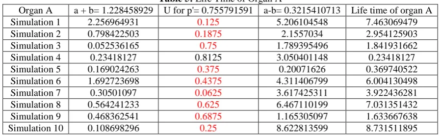
(vii) Results for Special case (2):
The following table 5 gives the failure times of the organ A in fifth column. Exponential random times are simulated using inverse method described earlier. The Organ A failure time is simulated using (40) and (41). It may be noted that the second exponential simulated value in column 4 is added to the first exponential simulated value in column 2 when u value in column 3 is u ≤ p' = 0.755791591 presented in red color.
Table 5: Life Time of Organ A
Organ A a + b= 1.228458929 U for p'= 0.755791591 a-b= 0.3215410713 Life time of organ A
Simulation 1 2.256964931 0.125 5.206104548 7.463069479
Simulation 2 0.798422503 0.1875 2.1557034 2.954125903
Simulation 3 0.052536165 0.75 1.789395496 1.841931662
Simulation 4 0.23418127 0.8125 3.050401148 0.23418127
Simulation 5 0.169024263 0.375 0.20071626 0.369740522
Simulation 6 1.692723698 0.4375 4.311406799 6.004130498
Simulation 7 0.30501097 0.0625 3.617425311 3.922436281
Simulation 8 0.564241233 0.625 6.467110199 7.031351432
Simulation 9 0.468362541 0.6875 1.165305097 1.633667638
© 2016, IJMA. All Rights Reserved 25
Simulation 11 0.672939529 0.3125 0.415285649 1.088225179
Simulation 12 1.128482466 0.875 2.570989049 1.128482466
Simulation 13 0.94683736 0.9375 0.894697748 0.94683736
Simulation 14 0.382596128 0.5 0.645763118 1.028359246
Simulation 15 1.362663736 0.5625 1.461721911 2.824385647
Failure time of the Organ B is given in Table 6 column 6 using the equations in (42), (43) and (44). Coxian simulated second exponential time in column 5 of table 6 is to be added with the sum of the terms of second and third columns when u value for 𝑝𝑝1is u ≤ 0.5 which is marked in red color. The maximum of the life time of the organ A (listed in table 5 column 5) and of the life time of the organ B (presented in column 6 table 6) may be seen in column 7 table 6 in red
color to indicate the maximum of the failure times of organ A and organ B.
Table 6: Life Time of Organ B and Maximum of Life Times of A and B
Organ B Erlang(5,2.5) Coxian Exp 1 U for 𝑝𝑝1=0.5 Coxian Exp 2 Life time of B Max(A,B) Simulation 1 2.020040071 0.028768207 0.625 0.012489782 2.048808278 7.463069479 Simulation 2 0.812358219 0.103972077 0.9375 0.046209812 0.916330296 2.954125903 Simulation 3 1.830256879 0.003226926 0.75 0.019178805 1.833483805 1.841931662 Simulation 4 1.075070034 0.05815754 0.0625 0.015666788 1.148894362 1.148894362 Simulation 5 1.996463057 0.00667657 0.875 0.027555952 2.003139626 2.003139626 Simulation 6 3.467994704 0.018734672 0.1875 0.038771694 3.52550107 6.004130498 Simulation 7 2.206900295 0.014384104 0.3125 0.032694308 2.253978707 3.922436281 Simulation 8 0.516491341 0.138629436 0.125 0.055799214 0.710919991 7.031351432 Simulation 9 2.180444374 0.023500181 0.4375 0.009589402 2.213533958 2.213533958 Simulation 10 1.857854028 0.041333929 0.25 0.092419624 1.991607581 8.731511895 Simulation 11 2.018258331 0.034657359 0.5625 0.069314718 2.05291569 2.05291569 Simulation 12 2.798404131 0.010381968 0.375 0.002151284 2.810937383 2.810937383 Simulation 13 0.928339108 0.049041463 0.6875 0.023104906 0.97738057 0.97738057 Simulation 14 0.99922169 0.083698822 0.5 0.006921312 1.089841824 1.089841824 Simulation 15 2.671022638 0.069314718 0.8125 0.004451046 2.740337356 2.824385647
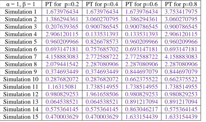
Time to Prophylactic treatment for the type (i) when α = 0.5 ≠ β = 1 using (45) and (46) for Coxian exponential times 1 and 2 are presented in columns 2 and 7 of table 7. The column 7 of table 7 is added with column 2 when u values in the columns 3 to 6 are not greater than p = 0.2, 0.4, 0.6, 0.8 by purple color.
Table 7: Simulated Random Values for Components of Time to Prophylactic Treatment for Type (i) α = 0.5, β = 1 Cox 1 (Para 0.5) U for p =0.2 U for p=0.4 U for p=0.6 U for p=0.8 Cox 2 (Para 1)
Simulation 1 0.575364145 0.8125 0.875 0.9375 0.0625 2.079441542
Simulation 2 3.347952867 0.5 0.3125 0.625 0.625 1.673976434
Simulation 3 0.940007258 0.9375 0.25 0.5625 0.1875 0.693147181
Simulation 4 5.545177444 0.125 0.6875 0.75 0.75 2.772588722
Simulation 5 1.386294361 0.0625 0.625 0.1875 0.3125 0.133531393
Simulation 6 0.129077042 0.75 0.0625 0.875 0.875 0.064538521
Simulation 7 1.961658506 0.1875 0.4375 0.8125 0.4375 1.386294361
Simulation 8 0.41527873 0.375 0.375 0.4375 0.5625 0.207639365
Simulation 9 2.772588722 0.3125 0.8125 0.125 0.125 0.470003629 Simulation 10 0.749386899 0.4375 0.75 0.0625 0.6875 0.374693449
Simulation 11 4.158883083 0.625 0.1875 0.25 0.25 0.575364145
Simulation 12 1.15072829 0.5625 0.125 0.6875 0.8125 0.980829253
Simulation 13 1.653357146 0.25 0.5625 0.375 0.375 0.826678573
Simulation 14 0.267062785 0.6875 0.5 0.3125 0.9375 0.287682072
Simulation 15 2.32630162 0.875 0.9375 0.5 0.5 1.16315081
Table 8: Simulated Times for Prophylactic Treatment (PT) for Type (i) for Values of p
α = 0.5, β = 1 PT for p=0.2 PT for p=0.4 PT for p=0.6 PT for p=0.8
Simulation 1 0.575364145 0.575364145 0.575364145 2.654805687 Simulation 2 3.347952867 5.021929301 3.347952867 5.021929301 Simulation 3 0.940007258 1.633154439 0.940007258 0.940007258 Simulation 4 8.317766167 5.545177444 5.545177444 8.317766167 Simulation 5 1.519825754 1.386294361 1.519825754 1.519825754 Simulation 6 0.129077042 0.129077042 0.129077042 0.193615563 Simulation 7 3.347952867 1.961658506 1.961658506 3.347952867 Simulation 8 0.41527873 0.622918094 0.622918094 0.622918094 Simulation 9 2.772588722 2.772588722 3.242592351 3.242592351 Simulation 10 0.749386899 0.749386899 1.124080348 1.124080348 Simulation 11 4.158883083 4.734247228 4.734247228 4.734247228 Simulation 12 1.15072829 2.131557543 1.15072829 1.15072829 Simulation 13 1.653357146 1.653357146 2.48003572 2.48003572 Simulation 14 0.267062785 0.267062785 0.554744858 0.267062785 Simulation 15 2.32630162 2.32630162 3.489452429 3.489452429
Table 9:Time to Hospitalization T for different p values for Type (i)
(α, β) = (0.5, 1) T for p =0.2 T for p=0.4 T for p=0.6 T for p=0.8
Simulation 1 0.575364145 0.575364145 0.575364145 2.654805687 Simulation 2 2.954125903 2.954125903 2.954125903 2.954125903 Simulation 3 0.940007258 1.633154439 0.940007258 0.940007258 Simulation 4 1.148894362 1.148894362 1.148894362 1.148894362 Simulation 5 1.519825754 1.386294361 1.519825754 1.519825754 Simulation 6 0.129077042 0.129077042 0.129077042 0.193615563 Simulation 7 3.347952867 1.961658506 1.961658506 3.347952867 Simulation 8 0.41527873 0.622918094 0.622918094 0.622918094 Simulation 9 2.213533958 2.213533958 2.213533958 2.213533958 Simulation 10 0.749386899 0.749386899 1.124080348 1.124080348 Simulation 11 2.05291569 2.05291569 2.05291569 2.05291569 Simulation 12 1.15072829 2.131557543 1.15072829 1.15072829 Simulation 13 0.97738057 0.97738057 0.97738057 0.97738057 Simulation 14 0.267062785 0.267062785 0.554744858 0.267062785 Simulation 15 2.32630162 2.32630162 2.824385647 2.824385647
Time to Prophylactic treatment for the type (ii) when α = β = 1 using (47) and (48) for Coxian exponential times 1 and 2 are presented in columns 2 and 7 of table 10. The column 7 is considered for addition when u values in the columns 3 to 6 are not greater than p = 0.2, 0.4, 0.6 and 0.8 by purple color.
Table 10: Simulated Values for the Components of Time to Prophylactic Treatment for Type (ii) and u values
α = 1, β = 1 Cox 1 (Para 1) U for p =0.2 U for p=0.4 U for p=0.6 U for p=0.8 Cox 2 (Para 1)
Simulation 1 1.673976434 0.8125 0.875 0.9375 0.0625 2.079441542
Simulation 2 1.386294361 0.5 0.3125 0.625 0.625 1.673976434
Simulation 3 0.207639365 0.9375 0.25 0.5625 0.1875 0.693147181
Simulation 4 0.133531393 0.125 0.6875 0.75 0.75 2.772588722
Simulation 5 0.826678573 0.0625 0.625 0.1875 0.3125 0.133531393
Simulation 6 0.693147181 0.75 0.0625 0.875 0.875 0.064538521
Simulation 7 2.772588722 0.1875 0.4375 0.8125 0.4375 1.386294361 Simulation 8 2.079441542 0.375 0.375 0.4375 0.5625 0.207639365 Simulation 9 0.374693449 0.3125 0.8125 0.125 0.125 0.470003629 Simulation 10 0.287682072 0.4375 0.75 0.0625 0.6875 0.374693449
Simulation 11 1.16315081 0.625 0.1875 0.25 0.25 0.575364145
Simulation 12 0.980829253 0.5625 0.125 0.6875 0.8125 0.980829253
Simulation 13 0.064538521 0.25 0.5625 0.375 0.375 0.826678573
Simulation 14 0.575364145 0.6875 0.5 0.3125 0.9375 0.287682072
© 2016, IJMA. All Rights Reserved 27 Using table 10, simulated times for prophylactic treatment are presented below in table 11 considering addition where ever second observations are required for type (ii). Time to hospitalization for treatment is presented below for α = 1 = β in table 12. The Red colorindicates the patient is admitted due to the failures of organs A and B. The purple color is for prophylactic treatment. The hospital treatment times may be simulated as follows. Since the treatment time 𝐻𝐻1is the sum of Erlang random variable with parameter set (2,60) and three exponential random variables with
parameters c, d and 60 where c=132.9150262213 and d =27.0849737787 by equation (49), the simulated 𝐻𝐻1values are presented as follows in table 13. The total treatment time for 𝐻𝐻1 is given in column 6 table 13 by adding the columns 2 to 5 in table 13. The treatment times 𝐻𝐻2 is generated by LCGs as mentioned in (vi) earlier and presented in column 7 of table 13. The red and purple colors indicate the treatment times are for the organs A and B and for prophylactic treatment respectively.
Table 11: Simulated Times for Prophylactic Treatment (PT) for Type (ii) for Values of p
α = 1, β = 1 PT for p=0.2 PT for p=0.4 PT for p=0.6 PT for p=0.8
Simulation 1 1.673976434 1.673976434 1.673976434 3.753417975 Simulation 2 1.386294361 3.060270795 1.386294361 3.060270795 Simulation 3 0.207639365 0.900786545 0.900786545 0.900786545 Simulation 4 2.906120115 0.133531393 0.133531393 2.906120115 Simulation 5 0.960209966 0.826678573 0.960209966 0.960209966 Simulation 6 0.693147181 0.757685702 0.693147181 0.693147181 Simulation 7 4.158883083 2.772588722 2.772588722 4.158883083 Simulation 8 2.079441542 2.287080906 2.287080906 2.287080906 Simulation 9 0.374693449 0.374693449 0.844697079 0.844697079 Simulation 10 0.287682072 0.287682072 0.662375522 0.662375522 Simulation 11 1.16315081 1.738514955 1.738514955 1.738514955 Simulation 12 0.980829253 1.961658506 0.980829253 0.980829253 Simulation 13 0.064538521 0.064538521 0.891217094 0.891217094 Simulation 14 0.575364145 0.575364145 0.863046217 0.575364145 Simulation 15 0.470003629 0.470003629 1.633154439 1.633154439
Table 12: Simulated Times for Time to Hospitalization T for Type (ii)
α = 1, β = 1 T for p = 0.2 T for p=0.4 T for p=0.6 T for p=0.8
Simulation 1 1.673976434 1.673976434 1.673976434 3.753417975 Simulation 2 1.386294361 2.954125903 1.386294361 2.954125903 Simulation 3 0.207639365 0.900786545 0.900786545 0.900786545 Simulation 4 1.148894362 0.133531393 0.133531393 1.148894362 Simulation 5 0.960209966 0.826678573 0.960209966 0.960209966 Simulation 6 0.693147181 0.757685702 0.693147181 0.693147181 Simulation 7 3.922436281 2.772588722 2.772588722 3.922436281 Simulation 8 2.079441542 2.287080906 2.287080906 2.287080906 Simulation 9 0.374693449 0.374693449 0.844697079 0.844697079 Simulation 10 0.287682072 0.287682072 0.662375522 0.662375522 Simulation 11 1.16315081 1.738514955 1.738514955 1.738514955 Simulation 12 0.980829253 1.961658506 0.980829253 0.980829253 Simulation 13 0.064538521 0.064538521 0.891217094 0.891217094 Simulation 14 0.575364145 0.575364145 0.863046217 0.575364145 Simulation 15 0.470003629 0.470003629 1.633154439 1.633154439
Table 13: Hospital Treatment Times for Stage Treatments Type 𝐻𝐻1,Total of 𝐻𝐻1 and 𝐻𝐻2
Simulation 12 0.021141855 0.015644894 0.013833997 0.023104906 0.073725653 0.035389346 Simulation 13 0.069314718 0.008751086 0.004930091 0.001075642 0.084071537 0.067351667 Simulation 14 0.017422796 0.01042993 0.021242928 0.002225523 0.051321177 0.015459746 Simulation 15 0.02161137 0.000485562 0.010621464 0.046209812 0.078928208 0.016609627
The simulated values in table 13 are common for the two types (i) and (ii). They are to be linked to table 9 and table 12 for the types (i) and (ii). For example in table 9 type (i), the patient is admitted for prophylactic treatment for p=0.2 in simulation 1 at time 0.575364145 and he is to be provided treatment 𝐻𝐻2 for time 0.023667687 given for simulation 1 column 7 in table 13. Similarly in simulation 4 for p = 0.2 in table 12 the organs A and B are in failed state at time
1.148894362 and his hospital treatment time for 𝐻𝐻1is to be 0.131681178. For the fifteen simulations of time to hospitalization T in table 9 for various values of p the corresponding treatment types and times are listed in table 14. Purple color indicates the prophylactic treatment and red color indicates the treatment times of organs A and B. The simulated values of table 13 are to be linked to table 12 for type (ii). For example in table 12 simulation 7 for p = 0.2 , the patient is admitted for hospitalization due to the failure of the organs at time 3.922436281 and he is to be provided treatment 𝐻𝐻1 for time0.156610868 which is placed in table 13 simulation 7 column 6. In similar manner all the fifteen simulations of table 12 for various values of p may be linked with corresponding simulated treatment times in table 13. They are presented in table 15 for type (ii).
Table 14: Hospital treatment times H for Type (i)-Unequal rates (α, β) = (0.5, 1) (α, β) = (0.5, 1) H time p=0.2 H time p=0.4 H time p=0.6 H time p=0.8 Simulation 1 0.023667687 0.023667687 0.023667687 0.023667687 Simulation 2 0.059286895 0.059286895 0.059286895 0.059286895 Simulation 3 0.074109419 0.074109419 0.074109419 0.074109419 Simulation 4 0.131681178 0.131681178 0.131681178 0.131681178 Simulation 5 0.047285454 0.047285454 0.047285454 0.047285454 Simulation 6 0.066232679 0.066232679 0.066232679 0.066232679 Simulation 7 0.062556966 0.062556966 0.062556966 0.062556966 Simulation 8 0.120319231 0.120319231 0.120319231 0.120319231 Simulation 9 0.040570644 0.040570644 0.040570644 0.040570644 Simulation 10 0.039408714 0.039408714 0.039408714 0.039408714 Simulation 11 0.022416335 0.022416335 0.022416335 0.022416335 Simulation 12 0.035389346 0.035389346 0.035389346 0.035389346 Simulation 13 0.084071537 0.084071537 0.084071537 0.084071537 Simulation 14 0.015459746 0.015459746 0.015459746 0.015459746 Simulation 15 0.016609627 0.016609627 0.078928208 0.078928208
Table 15: Hospital treatment times for Type (ii)-Equal rates (α, β) = (1, 1)
(α, β) = (1, 1) H time p=0.2 H time p=0.4 H time p=o.6 H time p=0.8
Simulation 1 0.023667687 0.023667687 0.023667687 0.023667687 Simulation 2 0.020883452 0.059286895 0.020883452 0.059286895 Simulation 3 0.074109419 0.074109419 0.074109419 0.074109419 Simulation 4 0.131681178 0.023922145 0.023922145 0.131681178 Simulation 5 0.047285454 0.047285454 0.047285454 0.047285454 Simulation 6 0.066232679 0.066232679 0.066232679 0.066232679 Simulation 7 0.156610868 0.062556966 0.062556966 0.156610868 Simulation 8 0.120319231 0.120319231 0.120319231 0.120319231 Simulation 9 0.048435335 0.048435335 0.048435335 0.048435335 Simulation 10 0.039408714 0.039408714 0.039408714 0.039408714 Simulation 11 0.022846503 0.022846503 0.022846503 0.022846503 Simulation 12 0.035389346 0.035389346 0.035389346 0.035389346 Simulation 13 0.067351667 0.067351667 0.067351667 0.067351667 Simulation 14 0.015459746 0.015459746 0.015459746 0.015459746 Simulation 15 0.016609627 0.016609627 0.016609627 0.016609627
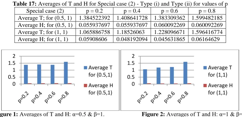
© 2016, IJMA. All Rights Reserved 29 Table 17: Averages of T and H for Special case (2) - Type (i) and Type (ii) for values of p
Special case (2) p = 0.2 p = 0.4 p = 0.6 p = 0.8 Average T; for (0.5, 1) 1.384522392 1.408641728 1.383309362 1.599482185 Average H; for (0.5, 1) 0.055937697 0.055937697 0.060092269 0.060092269 Average T; for (1, 1) 1.065886758 1.18526063 1.228096671 1.596416774 Average H; for (1, 1) 0.05908606 0.048192094 0.045631865 0.06164629
Figure 1: Averages of T and H: α=0.5 & β=1. Figure 2: Averages of T and H: α=1 & β=1
In the type (i) and type (ii), the only difference is in the value of the parameter α where in type (i) α = 0.5 and in type (ii) α =1. The effect of the change of α, the parameter of the first exponential observation time, may be seen on comparing figures (1) and (2) for averages. The variations of average of simulated values are comparatively high for p = 0.8 when the second prophylactic observation is taken up in 80% of the cases. Both the averages T and H are more for p = 0.8 compared to p = 0.6. In the last column of table 15, corresponding to simulations 2, 4 and 7, it may be noted that the two organs fail before the completion of second observation time calling for treatment of type 𝐻𝐻1. Possibly the second observation may not be required in those cases. This actually increases both the averages of T and H for p = 0.8 which is exhibited in figure 2. In the other figure also variations of E(T) and E(H) can be noted.
CONCLUSION
Diabetic models with two observation times including one for second opinion for prophylactic treatment have been studied with two defective organs exposed to failures. Two types have come up depending on whether the observation holding time rates are equal or not equal. In the model the patient has been sent for hospitalization when both organs have failed or when prophylactic treatment has started. The organ A of the patient has two phase PH life distribution and his organ B has general life time. The time to prophylactic treatment has Coxian 2 distribution. The hospital treatment times for the organs A and B and for prophylactic treatments have distinct distributions 𝐻𝐻𝑤𝑤 for i=1 and 2 respectively. The joint Laplace Stieltjes transform of the joint distribution of time to hospitalization and hospitalization time have been obtained. Individual distributions are also presented. The expected time to hospitalization and the expected hospitalization times are derived. Numerical studies are presented for the two models assuming exponential life time distribution for organ B by fixing and varying parameter values. Simulation study has been taken up in this area considering a set of parameter values of two phase life distribution of the organ A. EC distribution is the closed form approximation for the general life time distribution of the organ B. Different parameter values of Coxian time to prophylactic treatment, Erlang and cyclic phase type distributions for hospitalization times for the two cases of the model are taken up for simulation. Cyclic type treatment in the hospital for 𝐻𝐻1 has been identified as acyclic type using equality of distributions so that simulation can be performed easily. All the results are tabulated and graphical presentation are provided. Since not much of simulation analysis are available in literature for diabetic models, this study opens up a real life like study in this area. Various other distributions if used for simulation studies may also produce more interesting results.
REFERENCES
1. Bhattacharya S.K., Biswas R., Ghosh M.M., Banerjee., (1993), A Study of Risk Factors of Diabetes Mellitus, Indian Community Med., 18, pp.7-13.
2. Foster D.W., Fauci A.S., Braunward E., Isselbacher K.J., Wilson J.S., Mortin J.B., Kasper D.L., (2002),
Diabetes Mellitus, Principles of International Medicines,2, 15th edition pp.2111-2126. 3. Kannell W.B., McGee D.L.,(1979), Diabetes and Cardiovascular Risk Factors- the Framingam Study,
Circulation,59,pp. 8-13.
4. King H, Aubert R.E., Herman W.H., (1998), Global Burdon of Diabetes 1995-2025: Prevalence, Numerical Estimates and Projections, Diabetes Care 21, p 1414-1431.
5. King H and Rewers M,(1993), Global Estimates for Prevalence of Diabetes Mellitus and Impaired Glucose Tolerance in Adults: WHO Ad Hoc Diabetes Reporting Group, Diabetes Care, 16, p157-177.
6. Usha K and Eswariprem., (2009), Stochastic Analysis of Time to Carbohydrate Metabolic Disorder, International Journal of Applied Mathematics, 22,2, p317-330.
0 0.51 1.52
Average T
for (0.5,1)
Average H
for (0.5,1)
0 0.51 1.52
Average T
for (1,1)
Average H
7. Eswari Prem, Ramanarayanan R and Usha K., (2015),Stochastic Analysis of Prophylactic Treatment of a Diabetic Person with Erlang-2,IOSR Journal of Mathematics Vol. 11, Issue 5, Ver. 1 p01-07
8. Rajkumar A, Gajivaradhan P and Ramanarayanan R, (2015), Stochastic Analysis and Simulation Studies of Time to Hospitalization and Hospitalization Time with Prophylactic Treatment for Diabetic Patient with Two Failing Organs, IOSRJM, Vol. 11, Issue 6, Ver. III, pp.01-12.
9. Raja Rao B., (1998), Life Expectancy for Setting the Clock Back to Zero Property, Mathematical Biosciences, pp.251-271.
10. Murthy S and Ramanarayanan. R., (2009), Two (s, S) Inventory System with Binary Choice of Demands and Optional Accessories with SCBZ Arrival Property, Int.J.Contemp.Math.Sciences, Vo;. 4, No.9, pp. 397-417. 11. Snehalatha M, Sekar P and Ramanarayanan R., (2015) Probabilistic Analysis of General Manpower- SCBZ
Machine System with Exponential Production, General Sales and General Recruitment, IOSR Journal of Mathematics, IOSR-JM, Vol.11, Issue 2, Ver., VI, Mar- Apr, pp.12-21.
12. T.Osogami and M.H.Balter.,(2003), A closed-Form Solution for Mapping General Distributions to Minimal PH Distributions, http://repository.cmu.edu/compsci.
13. Martin Haugh (2004) Generating Random Variables and Stochastic Processes, Monte Carlo Simulation: IEOR EA703
14. T.E. Hull and A.R. Dobell, (1962), Random Number Generators, Siam Review 4, No.3. Pp.230-249.
15. Mark Fackrell, (2009) Modeling Healthcare Systems with Phase-Type Distributions, Health Care Management Sci,12, p11-26, DOI 10,1007/s10729-008-9070-y.
Source of support: Nil, Conflict of interest: None Declared