R E S E A R C H
Open Access
Phase diagram of a QED-cavity array coupled
via a
N
-type level scheme
Jiasen Jin
1*, Rosario Fazio
1,2and Davide Rossini
1*Correspondence: [email protected] 1NEST, Scuola Normale Superiore
and Istituto di Nanoscienze, CNR, Piazza dei Cavalieri, 7, Pisa, 56126, Italy
Full list of author information is available at the end of the article
Abstract
We study the zero-temperature phase diagram of a one-dimensional array of QED cavities where, besides the single-photon hopping, an additional coupling between neighboring cavities is mediated by anN-type four-level system. By varying the relative strength of the various couplings, the array is shown to exhibit a variety of quantum phases including a polaritonic Mott insulator, a density-wave and a superfluid phase. Our results have been obtained by means of numerical
density-matrix renormalization group calculations. The phase diagram was obtained by analyzing the energy gaps for the polaritons, as well as through a study of two-point correlation functions.
PACS Codes: 42.50.Pq; 85.25.Cp; 64.70.Tg
Keywords: cavity quantum electrodynamics; strongly correlated polariton systems; quantum phase transitions
1 Introduction
The recent impressive advances in the field of quantum simulators allowed to probe the many-body physics of strongly correlated systems at the level of the single quantum ob-ject. At present cold atoms trapped in optical lattices can be considered among the most promising examples of quantum simulators. By means of ultracold atomic and molecular gases, it is nowadays possible to reach a degree of control and accuracy in engineering the dynamics of many-body systems that were unimaginable in previously. As a consequence, the coherent quantum dynamics emerging from carefully tailored microscopic Hamilto-nians can now be tested experimentally []. It has been possible, just to recall one example, to implement the Bose-Hubbard (BH) model [, ] and to detect its zero-temperature su-perfluid (SF) to Mott insulator (MI) quantum phase transition []. Other models involving spinor gases, Fermi systems, Bose-Fermi mixtures, or dipolar gases have been also devised and realized, providing an even richer phase diagram (see for example the review []). We mention the stabilization of density-wave (DW) phases for bosons, as well as more pe-culiar topological or supersolid orderings, which can arise in the presence of finite-range interactions [].
More recently a novel kind of many-body quantum simulator has been introduced, based on the idea to use single photons as quantum objects. Since photons hardly in-teract in open space, the most natural way to significantly increase their inin-teractions is to trap them into an optical QED cavity, and couple the field with atoms/molecules
side it in order to create an optical nonlinearity. If the nonlinearity is sufficiently large, the so called photon blockade sets in [, ], namely, the presence of a single photon inside a cavity prevents a second one to enter it. In the rotating-wave approximation, the simplest light-matter interaction scheme of this type can be accurately described by the Jaynes-Cummings (JC) model. By arranging an array of cavities coupled through the photon hop-ping, such to generate a competition between the hopping and the on-site nonlinearities, one can devise a setup that is well described by the so called Jaynes-Cummings-Hubbard (JCH) model [–].
In many respects, if one ignores dissipation, the physics emerging from the JCH Hamil-tonian resembles, at low-energies, that of an effective BH model. Probably the main differ-ence between the two systems is that, instead of having neutral bosons as building blocks of the model, in the JCH Hamiltonian one has to think in terms of polaritons,i.e., combined photonic/atomic excitations. Many different works already addressed the JCH equilibrium phase diagram with analytical, as well as numerical methods, leading to a fairly complete theoretical understanding of the nature and the location of the emerging phases and phase transitions in terms of the parameters governing the system (the field has been recently reviewed in,e.g., Refs. [–]).
Additional interest in cavity arrays comes from the fact that these systems can be nat-urally considered as open-system quantum simulators. Some related features have been recently explored [–]. In the following we will not touch on this and consider only the ‘equilibrium’ phase diagram.
This intense activity has been very recently boosted by the first experiments on QED cavity arrays [–]. As of today, the most concrete possibility to realize controllable and scalable quantum simulators with cavity arrays involves circuit-QED cavities [–].
So far the coupling between cavities has been mostly considered through photon hop-ping. Only few works started addressing more general schemes, where the cavity coupling can be induced also by means of non-linear elements [, , , ]. Such configurations include cross-Kerr interactions and/or correlated hopping terms, which lead to gener-alizations of the JCH model in a way similar to the extended BH (EBH) Hamiltonian for atoms with large dipole momentum loaded in optical lattices []. The underlying physical model is believed to possess a much richer structure, with the emergence of exotic phases of correlated polaritons. It is particularly interesting to address these schemes in one-dimensional (D) systems, where interactions become crucial to stabilize exotic phases of matter [–]. These notably include a series of nontrivial density-wave (DW) states, which can arise in the strong coupling regime [], as well as supersolidity and phase-separation effects [, ]. Extension to consider also counter-rotating terms in the ultra-strong coupling regime, thus leading to the so called Rabi-Hubbard model [], have been investigated []. However we are not aware of numerical investigations of coupled cavity models beyond the JCH and Rabi-Hubbard model.
Hilbert space of fixed dimensions, as the physical system grows. This truncation is per-formed by retaining the eigenstates corresponding to the mhighest eigenvalues of the reduced density matrix of the block.
The aim of this paper is to quantitatively study a generalization of the JCH Hamiltonian, aimed at taking into account an effective nearest-neighbor nonlinearity between cavities mediated by anN-type four-level system as discussed for two cavities in Ref. []. The presence of this coupling leads to an effective cross-Kerr nonlinearity. An analysis at the mean-field level of a dissipative open EBH as an effective model for nonlinearly coupled cavities has been performed, unveiling the emergence of novel photon crystal and super-solid phases [, ]. Here we do not resort to the effective EBH model and analyze the full model as introduced in []. Using the DMRG algorithm, we work out the D ground-state phase diagram. We show that a physics similar to the EBH model appears, with a rich phase diagram including gapless SF, as well as MI and DW phases of polaritons. We post-pone the analysis of the interplay of driving and dissipation to a future work.
The paper is organized as follows. In the next two sections we introduce the model of coupled cavities of our interest (Section ) and the quantities we are going to address, namely the energy gaps, and the staggered number-number correlations (Section ). In Section we discuss the zero-temperature equilibrium phase diagram, focusing on the MI/SF boundary and on the boundary separating the DW from the other phases. Finally, in Section we draw our conclusions.
2 The model
Let us consider a D array of QED cavities, where photons can hop between neighboring cavities. Moreover two adjacent resonators are also nonlinearly coupled to each other via a N-type four-level system, as shown in Figure (a). For the sake of clarity in our description, we shall divide the D array into coupled effective sites composed of a cavity and an atom. The four levels are denoted by{|i}i=,...,, and are depicted in Figure (b). An external laser
with frequencyresonantly drives the transition| ↔ |. The transition| ↔ |is resonantly coupled to the cavity mode of the same site with strengthg, while the transition
| ↔ |couples to the cavity mode of its right nearest-neighbor site with strengthg, and
a detuning.
The use of suchN-type atom for generating large Kerr nonlinearity has been extensively studied in the literature [, , ], however the vast majority of the scenarios only focused on a single-mode cavity. Our work is inspired by the idea of Ref. [], where the cross-Kerr
Figure 1 Scheme for nonlinearly coupled QED cavities. (a)An array of QED cavities nonlinearly coupled byN-type atoms. The photon hopping between nearest-neighbor cavities has a strengtht. Each effective site is composed of a cavity and an atom (dashed box).(b)Level structure of theN-type atoms. The transition|1 ↔ |3is resonantly coupled to the cavity mode of its own site with strengthg1, while|2 ↔ |4is coupled to the cavity mode of its right nearest-neighbor site with strength
nonlinearity is generated between two different and neighboring cavities, in circuit-QED systems. In practice, we use the unbalanced couplings of atomic transition| ↔ |with left cavity mode, and| ↔ |with right cavity mode respectively, in order to generate the local (g) and nonlocal (g) nonlinearities of our many-body system. This kind of
four-level artificial molecule can be realized using two Josephson transmon qubits coupled by a superconducting quantum interference device.
Using the interaction picture and in the rotating-wave approximation, the system Hamil-tonian reads
H=
i
σi+σi+gσia † i + H.c.
+–taia†i++gσia † i++ H.c.
, ()
whereσmn=|mn|(m,n= , , , ), anda(a†) is the annihilation (creation) operator of
the cavity mode. The subscripts denote the site position along the D chain. The first three terms in the r.h.s. of Eq. () describe the local terms and the nonlinearities on each site. Inside the latter brackets, the first term is the photon hopping, while the second term describes the coupling of the atom to its right neighboring cavity, which generates an ef-fective nonlocal cross-Kerr nonlinearity between the two cavities.
Hereafter we concentrate on the D model in Eq. () at zero temperature, specifically ad-dressing the case without dissipation with DMRG. Let us also fix the Hamiltonian quan-tities in units of, set= , and work with open boundary conditions. We recall that, in the presence of dissipation, the problem becomes much more difficult to be handled numerically.a
For the system we are considering here, in the strong coupling regime atoms and photons cannot be considered as two separate entities. It is thus natural to investigate the phase diagram in terms of combined atomic/photonic modes, named polaritons. The polaritonic number operator on each sitei, representing the number of local excitations, is defined as npoli = σi+σi+σi+a†iai. For the closed system described by the Hamiltonian (), the
total numberNpol=
in
pol
i of such polaritons is a conserved quantity. In the following we
work in the canonical ensemble for polaritons, and focus on the integer filling situation.
3 Energy gaps and correlation functions
The different nature of the various phases is sensitive to a number of properties which we are going to focus on. Here we are going to study quantities that resemble those charac-terizing the various phases of the EBH model [].
First of all, the ground-state energy gap is an important indicator which characterizes the presence or absence of criticality in the model. In particular, in the critical SF phase,
thecharge gapvanishes in the thermodynamic limit. On the other side, in the insulating
MI and DW phases, such gap remains finite. In order to make connection with a similar notation in the EBH model, below we introduce the so called charge and neutral gaps re-ferring respectively to the gaps corresponding to adding one extra particle (‘charge’ sector) or remaining with the same number of particles (‘neutral’ sector). We stress however that in the present model the excitation carry no real charge. This has to be understood only as a convention.
The charge gap is defined as
where, in the canonical ensemble,E+ (E–) denotes the extra energy needed to add
(remove) one particle,i.e.one polariton, in the system. In the specific, focusing on the unit filling,E+=EL+–ELandE–=EL–EL–, whereELis the ground-state energy per site
of anL-sites cavity-array with exactlyLexcitations, andEL+(EL–) is the corresponding
energy per site with one excitation more (less). It is therefore possible to extrapolateEc
by running three different DMRG simulations with fixed number of polaritonsNpol=L– , L,L+ [, ].
While the charge gap is able to detect particle-hole excitations, in some circumstances it is possible that the dominant low-energy excitations are of a different type. Their presence can be detected only by the so calledneutral gapat a fixed number of particles,
En=EL–EL, ()
where, again working in the canonical ensemble,EL denotes the first excited energy per site of anL-site system withLexcitations.
In the following, we also focus on the analysis of the staggered diagonal order for the po-laritons, in order to distinguish the DW from the other phases. We do this by investigating the two-point correlation function
CDW(r) = (–)r
δnpoli δnpoli+r, ()
whereδnpoli =npoli –n¯denotes the polariton fluctuation from the average fillingn¯. The or-der parameter identifying the DW phase is thus given by:ODW≡limr→∞CDW(r). A finite
value ofODWindicates a tendency to establish, in the thermodynamic limit, a staggered
occupation of the polaritons. On the other side, in the MI as well as the SF phases,CDW(r)
vanishes exponentially with increasing distancer.
4 Phase diagram
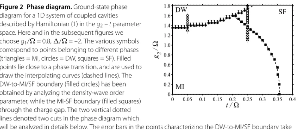
The zero-temperature phase diagram of model (), at unit polariton fillingn¯= and in theg–tplane, is summarized in Figure . We observe that three different phases can be
stabilized. Their boundaries have been obtained by means of a finite-size scaling of the numerical data, for systems up toL= sites. In our simulations we imposed a cutoff
Figure 2 Phase diagram.Ground-state phase diagram for a 1D system of coupled cavities described by Hamiltonian (1) in theg2–tparameter space. Here and in the subsequent figures we chooseg1/= 0.8,/= –2. The various symbols correspond to points belonging to different phases (triangles = MI, circles = DW, squares = SF). Filled points lie close to a phase transition, and are used to draw the interpolating curves (dashed lines). The DW-to-MI/SF boundary (filled circles) has been obtained by analyzing the density-wave order parameter, while the MI-SF boundary (filled squares) through the charge gap. The two vertical dotted lines denoted two cuts in the phase diagram which
photon number in each cavity, such thatnphoti ≤. We also truncated the effective Hilbert space dimension to a valuem= in all the simulations, except for those shown in Fig-ure for the neutral energy gap (see the discussion in Section .). We checked that, by increasingmand the local fock-space truncation over the photon number, the results con-cerning the charge gap and the DW order parameter do not change on the scales shown here.
For small photon hopping (t/.), by increasing the nonlocal nonlinearitygthe
system exhibits a direct transition from the MI to the DW phase. On the other hand, fort/., the MI-to-DW transition is mediated by an extended region appearing at intermediategvalues, where the system stabilizes into a gapless SF. In the following we
are going to elucidate our finite-size scaling procedure and how we were able to distinguish between the different phases.
4.1 Boundary between MI and SF phases
In the limit of smallg andtvalues, the dominant presence of the on-site interactions
stabilize the system into a MI phase with exactly one polariton per cavity (n¯= ), and where the charge energy gap has a finite value. As long as the hopping strengthtis progressively increased (and for fixedg,g), the system eventually enters a SF phase, with a vanishing
gap. The filled squares of Figure denoting the MI/SF boundaries have been obtained by means of a finite-size scaling of the charge gap. We performed simulations up toL= sites and analyzed whether the gap closes or remains finite in the thermodynamic limit
L→ ∞.
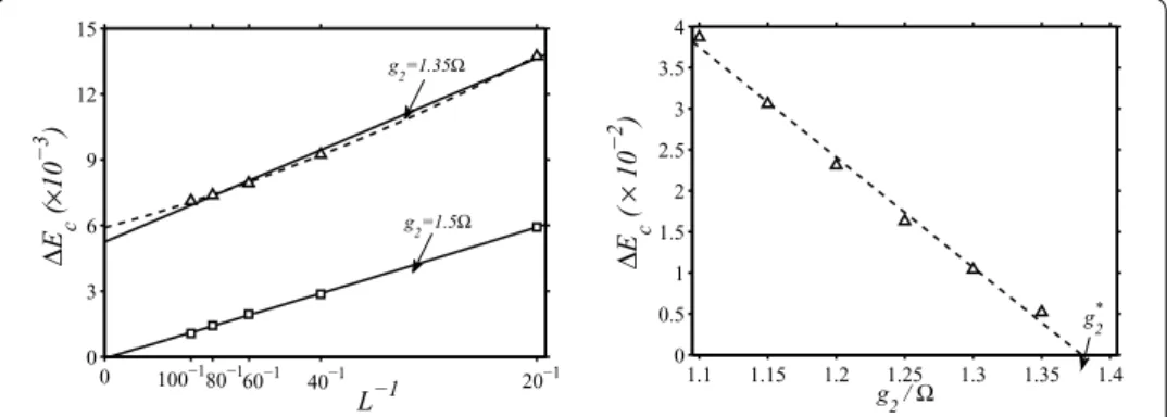
In Figure , left panel, we highlight the size-dependence ofEcas a function of /Lfor
two points in the phase space close to the MI/SF transition (see points along the dotted line in Figure ). We expect to see a quadratic dependenceEc∼L–(dashed line) at large
L[, ], however a linear extrapolation (solid line) is already a good approximation to the scaling, and we can use it to determineEcin the thermodynamics limit. Indeed, we
observe that the difference between quadratic and linear extrapolation is tiny (–) and
does not produce any distinguishable modification on the scale of Figure . In the specific case of Figure , we fixedt/= . and chose two different values ofg/corresponding
Figure 3 Analysis of the MI-SF boundary.Left panel: system-size dependence of the charge gapEcper site, for fixedt/= 0.25 and two values ofg2in the MI (g2/= 1.35) and in the SF (g2/= 1.5) phase. Symbols denote the DMRG results. Solid and dashed lines are linear and quadratic fitting curves, respectively. The difference between the extrapolated values in the two fitsEc∞= limL→∞E
(L)
to configurations in the gapped MI (g/= ., triangles) and in the gapless SF phase
(g/= ., squares). The MI is signaled by an extrapolated finite value oflimL→∞Ec> ,
while in the SF this is zero.
In order to locate the critical g for a given value oft(filled squares in Figure ) we
perform a linear extrapolation of the charge gaps in the vicinity of the critical value of g. An example of such procedure is shown in the right panel of Figure , where we plot
Ecas a function ofg, when this is close to the phase transition (in the specific, here
we sett/= .). After a linear extrapolation, we get a criticalg value corresponding
tog∗/≈.. An analogous procedure is repeated for all the filled squares shown in Figure , thus identifying the MI/SF boundary.
4.2 Boundary of the DW phase
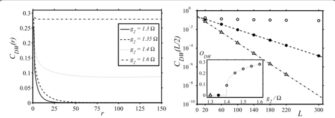
The DW phase is characterized by a finite order parameterODW. Let us therefore look at
the two-point staggered correlator in Eq. (). Since in DMRG simulations we are employ-ing open boundary conditions, to minimize the border effects we analyze the correlations in such a way that the two points are taken symmetrically with respect to the center of the system.bThe left panel of Figure shows how differently such polariton correlations
behave when the system goes from the MI to DW phase, for a fixed system size.
To be more accurate, in the right panel we performed a finite-size scaling and showed that the staggered correlationCDW(r) approaches the zero value exponentially withL, in
the MI phase (a similar behavior occurs in the SF region). On the other hand, in the DW such correlator asymptotically converges to a finite value. In the specific, here we fixt/= . and show that forg/= ., . the DW order is exponentially suppressed withL,
while forg/= . it remains finite. TheODWorder parameter reached forL→ ∞is
displayed in the inset as a function ofg.
In order to determine the DW boundary in the phase diagram of Figure , we adopted the following protocol. For a fixed value oft/, we start increasinggfrom zero up to a
finite value, with a fixed incrementδg= ., and to compute the DW order parameter
Figure 4 Determination of the DW boundaries.The two-point correlation functionCDW(r) for the polariton number and its asymptotic value near the MI-DW quantum phase transition. Here we fixt/= 0.05 and varyg2/. Left panel: behavior at fixed system sizeL= 300, as a function of the distancerand for different values ofg2/= 1.3, 1.35, 1.4, and 1.6. To minimize boundary effects, we chose the two points (i,i+r) symmetrically with respect to the center of the array. Right panel: finite-size scaling close to the transition. Empty circles, filled circles, and triangles respectively are forg2/= 1.4 (DW), 1.35 (near the critical point), and 1.3 (MI phase). In the MI phase,CDWvanishes exponentially withL, according to the fits:
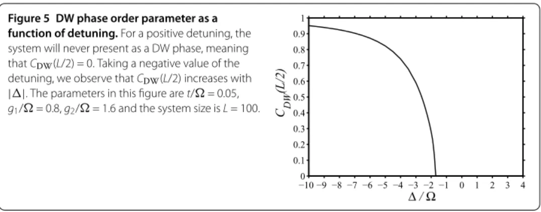
Figure 5 DW phase order parameter as a function of detuning.For a positive detuning, the system will never present as a DW phase, meaning thatCDW(L/2) = 0. Taking a negative value of the detuning, we observe thatCDW(L/2) increases with
||. The parameters in this figure aret/= 0.05,
g1/= 0.8,g2/= 1.6 and the system size isL= 100.
for all such values ofg. The boundary of DW phase in theg–tplane (filled circles in
Figure ), for any fixedt, is located by theg∗(t) that gives the first non-vanishing order parameterODW.
Here we stress that, because of the arrangement of our D array [see Figure (a)] and of the asymmetric coupling between the atom and its right/left cavity, the antiferromagnetic symmetry of the system is spontaneously broken. In particular, the state|of theL-th atom will be never occupied, since the transition| ↔ |does not couple to any cavity mode [see Eq. ()]. As a consequence, in our simulations we do not need any symmetry-breaking potential. We can observe that the expectation value for the onsite number of polaritons explicitly exhibits a staggered behavior, in that the occupation of the (n– )-th site is always higher than that of the (n)-th site (for any integer value ofn). Finally we no-tice that such staggering persists at finite size, also for the set of parameters corresponding to the MI phase, although it is extremely tiny and decreases withL. This effect eventually disappears in the thermodynamic limit.
The extension of the DW phase depends on the cavity detuning. In particular, the robustness of the order parameter increases with increasing the modulus of the detuning (see Figure ). Quite remarkably, we note that a positivewill never stabilize an antifer-romagnetic DW ordering.
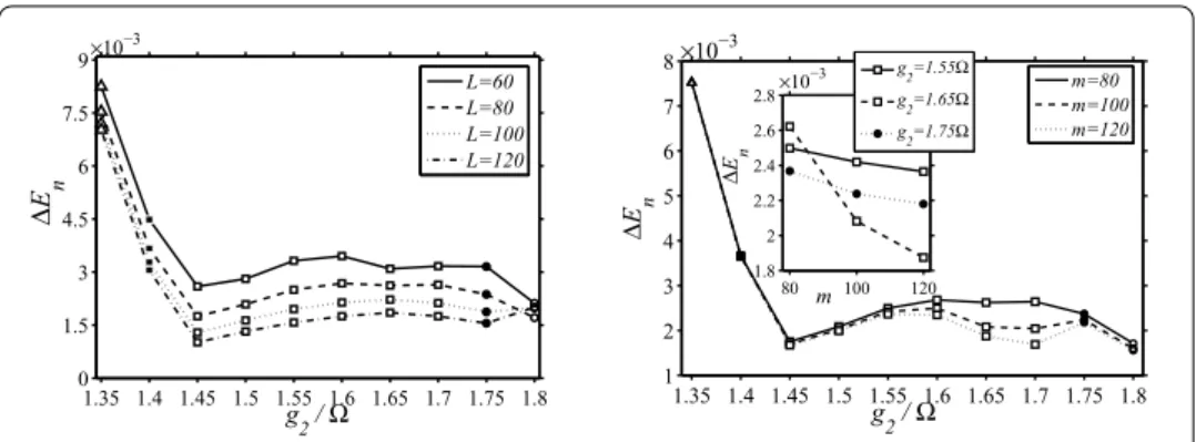
4.3 Neutral gap
The analysis leading to the phase diagram in Figure has been corroborated by a study of the neutral gap, which vanishes both in proximity of the phase transitions and in the entire superfluid region. Differently for the charge gap, it is able to detect the presence of excitations other than particle-hole, and thus locates the boundaries of insulating regions (as the DW) beyond the MI.
The data displayed in Figure show the behavior ofEnas a function ofg, for a fixed
value oft/. In particular we analyzed a vertical cut in the phase diagram of Figure (see the rightmost vertical dotted line in that figure), where the system can be in three different phases according to the value ofg. With increasingg, it goes from the MI phase (nonzero
En, fort/.) to the SF phase (zeroEn, for .t/.), and then to the DW
phase (nonzeroEn, fort/.).
While we cannot see a clear signature of a finite gap forg= ., the scaling with the
Figure 6 Analysis of the neutral gap.Neutral energy gap as a function ofg2fort/= 0.25,i.e., along the vertical cut depicted in Figure 2. In the left panel, the different curves are for various system sizes according to the legend, and for a fixed number of kept statesm= 80 in the DMRG algorithm. The right panel evidences the convergence of the data, at fixedL= 80, by increasingm(see also the inset, where we show the behavior ofEnas a function ofm, for three different values ofg2).
require a larger dimensionmof the effective Hilbert space, as compared to all the other ground-state calculations discussed before. The analysis of the neutral gap requires a care-ful convergence test of the results withm, which we provide in the right panel of Figure . We observe that the non monotonic features that are visible in the region .t/. have to be probably ascribed to the inaccuracy of the method at smallmvalues. This sig-nals the presence of the gapless SF phase there, in agreement with the results provided by the charge gap (MI/SF boundary) and for the DW order parameter (SF/DW boundary).
5 Summary
Using the density-matrix renormalization group with open boundary conditions, we stud-ied the equilibrium phase diagram of a system of coupled QED cavities in one dimension. We provided results beyond the standard model of couplings through photon hopping, and also considered nearest-neighbor cross-Kerr nonlinearities. Our analysis is based on a finite-size scaling of the ground-state charge and neutral gaps, as well as of the density-wave order parameter, for systems up to sites. We showed that, beyond the conven-tional Mott insulator and superfluid phases, the presence of a nearest-neighbor nonlinear coupling can also stabilize a density-wave ordering of polaritons.
Competing interests
The authors declare that they have no competing interests.
Authors’ contributions
All the authors participated in the design of the research, analysis of the results, and writing of the paper. The DMRG code used to run all the simulations of this research has been developed and written by DR and coworkers [44] (see also www.dmrg.it). The DMRG simulations were performed by JJ.
Author details
1NEST, Scuola Normale Superiore and Istituto di Nanoscienze, CNR, Piazza dei Cavalieri, 7, Pisa, 56126, Italy.2Center for
Quantum Technologies, National University of Singapore, Singapore, 117543, Singapore.
Acknowledgements
We would like to acknowledge our previous collaboration with M. Hartmann and M. Leib which was inspiring for the present work. This work was supported by Italian MIUR via FIRB Project RBFR12NLNA and PRIN Project 2010LLKJBX, by EU through IP-SIQS, and by National Natural Science Foundation of China under Grant No. 11175033 and No. 11305021.
Endnotes
a It is however possible to address the effect of dissipation with a DMRG approach in a 1D chain, when this is
generalize the matrix-product-state ansatz to a matrix-product-density-operator ansatz for mixed states, as originally proposed in Refs. [50, 51]. The computational complexity is greater than for static computations, and is eventually related to the amount of entanglement in the steady state.
b The two points ofδnpol i δn
pol
j , with|i–j|=r, have been chosen such thati= (L–r+ 1)/2,j= (L+r+ 1)/2 for oddr,
andi= (L–r)/2,j= (L+r)/2 for evenr(e.g.forL= 100 sites,r= 1 corresponds toi= 50,j= 51;r= 2 corresponds to
i= 49,j= 51;r= 3 toi= 49,j= 52, and so on).
Received: 31 July 2014 Accepted: 14 January 2015
References
1. Bloch I, Dalibard J, Zwerger W. Many-body physics with ultracold gases. Rev Mod Phys. 2008;80:885.
2. Fisher MPA, Weichman PB, Grinstein G, Fisher DS. Boson localization and the superfluid-insulator transition. Phys Rev B. 1989;40:546.
3. Jaksch D, Bruder C, Cirac JI, Gardiner CW, Zoller P. Cold bosonic atoms in optical lattices. Phys Rev Lett. 1998;81:3108. 4. Greiner M, Mandel O, Esslinger T, Hänsch TW, Bloch I. Quantum phase transition from a superfluid to a Mott insulator
in a gas of ultracold atoms. Nature. 2002;415:39.
5. Lewenstein M, Sanpera A, Ahufinger V, Damski B, Sen(De) A, Sen U. Ultracold atomic gases in optical lattices: mimicking condensed matter physics and beyond. Adv Phys. 2007;56:243.
6. Lahaye T, Menotti C, Santos L, Lewenstein M, Pfau T. The physics of dipolar bosonic quantum gases. Rep Prog Phys. 2009;72:126401.
7. Schmidt H, Imamo ˇglu A. Giant Kerr nonlinearities obtained by electromagnetically induced transparency. Opt Lett. 1996;21:1936.
8. Imamo ˇglu A, Schmidt H, Woods G, Deutsch M. Strongly interacting photons in a nonlinear cavity. Phys Rev Lett. 1997;79:1467.
9. Hartmann MJ, Brandão FGSL, Plenio MB. Strongly interacting polaritons in coupled arrays of cavities. Nat Phys. 2006;2:849.
10. Greentree AD, Tahan C, Cole JH, Hollenberg LCL. Quantum phase transitions of light. Nat Phys. 2006;2:856. 11. Angelakis DG, Santos MF, Bose S. Photon-blockade-induced Mott transitions and XY spin models in coupled cavity
arrays. Phys Rev A. 2007;76:031805(R).
12. Hartmann MJ, Brandão FGSL, Plenio MB. Quantum many-body phenomena in coupled cavity arrays. Laser Photonics Rev. 2008;2:527.
13. Tomadin A, Fazio R. Many-body phenomena in QED-cavity arrays. J Opt Soc Am. 2010;27:A130.
14. Houck AA, Türeci HE, Koch J. On-chip quantum simulation with superconducting circuits. Nat Phys. 2012;8:292. 15. Schmidt S, Koch J. Circuit QED lattices: towards quantum simulation with superconducting circuits. Ann Phys.
2013;525:395.
16. Carusotto I, Gerace D, De Liberato S, Ciuti C, Imamo ˇglu A. Fermionized photons in an array of driven dissipative nonlinear cavities. Phys Rev Lett. 2009;103:033601.
17. Tomadin A, Giovannetti V, Fazio R, Gerace D, Carusotto I, Türeci HE, Imamo ˇglu A. Signatures of the superfluid-insulator phase transition in laser-driven dissipative nonlinear cavity arrays. Phys Rev A. 2010;81:061801(R).
18. Hartmann MJ. Polariton crystallization in driven arrays of lossy nonlinear resonators. Phys Rev Lett. 2010;104:113601. 19. Nunnenkamp A, Koch J, Girvin SM. Synthetic gauge fields and homodyne transmission in Jaynes-Cummings lattices.
New J Phys. 2011;13:095008.
20. Nissen F, Schmidt S, Biondi M, Blatter G, Türeci HE, Keeling J. Nonequilibrium dynamics of coupled qubit-cavity arrays. Phys Rev Lett. 2012;108:233603.
21. Grujic T, Clark SR, Angelakis DG, Jaksch D. Non-equilibrium many-body effects in driven nonlinear resonator arrays. New J Phys. 2012;14:103025.
22. Grujic T, Clark SR, Jaksch D, Angelakis DG. Repulsively induced photon superbunching in driven resonator arrays. Phys Rev A. 2013;87:053846.
23. Jin J, Rossini D, Fazio R, Leib M, Hartmann MJ. Photon solid phases in driven arrays of nonlinearly coupled cavities. Phys Rev Lett. 2013;110:163605.
24. Jin J, Rossini D, Leib M, Hartmann MJ, Fazio R. Steady-state phase diagram of a driven QED-cavity array with cross-Kerr nonlinearities. Phys Rev A. 2014;90:023827.
25. Underwood DL, Shanks WE, Koch J, Houck AA. Low-disorder microwave cavity lattices for quantum simulation with photons. Phys Rev A. 2012;86:023837.
26. Abbarchi M, Amo A, Sala VG, Solnyshkov DD, Flayac H, Ferrier L, Sagnes I, Galopin E, Lemaître A, Malpuech G, Bloch J. Macroscopic quantum self-trapping and Josephson oscillations of exciton polaritons. Nat Phys. 2013;9:275. 27. Toyoda K, Matsuno Y, Noguchi A, Haze S, Urabe S. Experimental realization of a quantum phase transition of
polaritonic excitations. Phys Rev Lett. 2013;111:160501.
28. Lucero E, Barends R, Chen Y, Kelly J, Mariantoni M, Megrant A, O’Malley P, Sank D, Vainsencher A, Wenner J, White T, Yin Y, Cleland AN, Martinis JM. Computing prime factors with a Josephson phase qubit quantum processor. Nat Phys. 2012;8:719.
29. Steffen L, Salathe Y, Oppliger M, Kurpiers P, Baur M, Lang C, Eichler C, Puebla-Hellmann G, Fedorov A, Wallraff A. Deterministic quantum teleportation with feed-forward in a solid state system. Nature. 2013;500:319.
30. Chen Y, Roushan P, Sank D, Neill C, Lucero E, Mariantoni M, Barends R, Chiaro B, Kelly J, Megrant A, Mutus JY, O’Malley PJJ, Vainsencher A, Wenner J, White TC, Yin Y, Cleland AN, Martinis JM. Emulating weak localization using a solid-state quantum circuit. Nat Commun. 2014;5:5184.
31. Zueco D, Mazo JJ, Solano E, García Ripoll JJ. Microwave photonics with Josephson junction arrays: negative refraction index and entanglement through disorder. Phys Rev B. 2012;86:024503.
32. Peropadre B, Zueco D, Wulschner F, Deppe F, Marx A, Gross R, García Ripoll JJ. Tunable coupling engineering between superconducting resonators: from sidebands to effective gauge fields. Phys Rev B. 2013;87:134504.
34. Dalla Torre EG, Berg E, Altman E. Hidden order in 1D Bose insulators. Phys Rev Lett. 2006;97:260401. 35. Berg E, Dalla Torre EG, Giamarchi T, Altman E. Rise and fall of hidden string order of lattice bosons. Phys Rev B.
2008;77:245119.
36. Rossini D, Fazio R. Phase diagram of the extended Bose-Hubbard model. New J Phys. 2012;14:065012.
37. Deng X, Citro R, Orignac E, Minguzzi A, Santos L. Polar bosons in one-dimensional disordered optical lattices. Phys Rev B. 2013;87:195101.
38. Wikberg E, Larson J, Bergholtz EJ, Karlhede A. Fractional domain walls from on-site softening in dipolar bosons. Phys Rev A. 2012;85:033607.
39. Batrouni GG, Scalettar RT, Rousseau VG, Grémaud B. Competing supersolid and Haldane insulator phases in the extended one-dimensional bosonic Hubbard model. Phys Rev Lett. 2013;110:265303.
40. Batrouni GG, Rousseau VG, Scalettar RT, Grémaud B. Competing phases, phase separation, and coexistence in the extended one-dimensional bosonic Hubbard model. Phys Rev B. 2014;90:205123.
41. Schiró M, Bordyuh M, Öztop B, Türeci HE. Phase transition of light in cavity QED lattices. Phys Rev Lett. 2012;109:053601.
42. Kumar B, Jalal S. Quantum Ising dynamics and Majorana-like edge modes in the Rabi lattice model. Phys Rev A. 2013;88:011802(R).
43. Schollwöck U. The density-matrix renormalization group. Rev Mod Phys. 2005;77:259.
44. De Chiara G, Rizzi M, Rossini D, Montangero S. Density matrix renormalization group for dummies. J Comput Theor Nanosci. 2008;5:1277.
45. Rossini D, Fazio R. Mott-insulating and glassy phases of polaritons in 1D arrays of coupled cavities. Phys Rev Lett. 2007;99:186401.
46. Rossini D, Santoro GE, Fazio R. Photon and polariton fluctuations in arrays of QED-cavities. Europhys Lett. 2008;83:47011.
47. D’Souza AG, Sanders BC, Feder DL. Fermionized photons in the ground state of one-dimensional coupled cavities. Phys Rev A. 2013;88:063801.
48. Hu Y, Ge GQ, Chen S, Yang XF, Chen YL. Cross-Kerr-effect induced by coupled Josephson qubits in circuit quantum electrodynamics. Phys Rev A. 2011;84:012329.
49. Rebi´c S, Twamley J, Milburn GJ. Giant Kerr nonlinearities in circuit quantum electrodynamics. Phys Rev Lett. 2009;103:150503.
50. Verstraete F, García-Ripoll JJ, Cirac JI. Matrix product density operators: simulation of finite-temperature and dissipative systems. Phys Rev Lett. 2004;93:207204.
51. Zwolak M, Vidal G. Mixed-state dynamics in one-dimensional quantum lattice systems: a time-dependent superoperator renormalization algorithm. Phys Rev Lett. 2004;93:207205.
52. Kühner TD, Monien H. Phases of the one-dimensional Bose-Hubbard model. Phys Rev B. 1998;58:R14741.