AENSI Journals
Australian Journal of Basic and Applied Sciences
ISSN:1991-8178Journal home page: www.ajbasweb.com
Corresponding Author: Saadi bin Ahmad Kamaruddin,International Islamic University Malaysia, Computational and Theoretical Sciences Department, Kulliyyah of Science, Jalan Istana, Bandar Indera Mahkota, 25200 Kuantan, Pahang Darul Makmur, Malaysia.
Ph:+6 0176231710. E-mail:[email protected]
Comparative Study of Particle Swarm Optimization (PSO) and Firefly Algorithm (FA)
on Least Median Squares (LMedS) for Robust Backpropagation Neural Network
Learning Algorithm
1Saadi bin Ahmad Kamaruddin, 2Nor Azura Md. Ghani, 2Norazan Mohamed Ramli
1International Islamic University Malaysia, Computational and Theoretical Sciences Department, Kulliyyah of Science, Jalan Istana,
Bandar Indera Mahkota, 25200 Kuantan, Pahang Darul Makmur, Malaysia
2
Universiti Teknologi MARA, Center for Statistical and Decision Sciences Studies, Faculty of Computer and Mathematical Sciences, 40450 Shah Alam, Selangor Darul Ehsan, Malaysia
A R T I C L E I N F O A B S T R A C T Article history:
Received 30 September 2014 Received in revised form 17 November 2014 Accepted 25 November 2014 Available online 13 December 2014
Keywords:
Nonlinear time series, neural network, backpropagation learning, firefly algorithm, robust estimators
Background: There is no doubt that artificial neural network (ANN) is one of the most famous universal approximators, and has been implemented in many fields. This is due to its ability to automatically learn any pattern with no prior assumptions and loss of generality. ANNs have contributed significantly towards time series-prediction arena, but the presence of outliers that usually occur in the time series data may pollute the network training data. Theoretically, the most common algorithm to train the network is the backpropagation (BP) algorithm which is based on the minimization of the ordinary least squares (OLS) estimator in terms of mean squared error (MSE). However, this algorithm is not totally robust in the presence of outliers and may cause false prediction of future values. Objective: Therefore, in this paper, we implement a new algorithm which takes advantage of firefly algorithm on the least median of squares (FA-LMedS) estimator for artificial neural network nonlinear autoregressive (BPNN-NAR) and artificial neural network nonlinear autoregressive moving average (BPNN-NARMA) models to cater the various degrees of outlying problem in time series data.Moreover, the performance of the proposed robust estimator with comparison to the original MSE and robust particle swarm optimization on least median squares (PSO-LMedS) estimators using simulation data, based on root mean squared error (RMSE) are also discussed in this paper. Results: It was found that the robustified backpropagation learning algorithm using FA-LMedS outperformed the original and other robust estimator of PSO-LMedS. Conclusion: Evolutionary algorithms outperform the original MSE error function in providing robust training of artificial neural networks.
© 2014 AENSI Publisher All rights reserved. To Cite This Article: S.A.B. Kamaruddin, N.A.M. Ghani, N.M. Ramli., Comparative Study of Particle Swarm Optimization (PSO) and Firefly Algorithm (FA) on Least Median Squares (LMedS) for Robust Backpropagation Neural Network Learning Algorithm. Aust. J. Basic & Appl. Sci., 8(24): 117-129, 2014
INTRODUCTION
The backpropagation algorithm is based on the feedforward multilayer neural network for a set of inputs with specified known classifications. The algorithm allows multilayer feedforward neural networks to learn input-output mappings from training samples (Sibi et al., 2013). Once each entry of the sample set is presented to the network, its output response will be examined by the network with respect to the sample input pattern. The output response is then compared to the known and desired output and the error value is calculated, where the connection weights are adjusted. The backpropagation algorithm is based on Widrow-Hoff delta learning rule in which the weight adjustment is done through mean square error (MSE) of the output response to the sample input (Engelbrecht, 2007). The set of these sample patterns are repeatedly presented to the network until the error value is minimized.
algorithm is not completely robust in the presence of outliers. Even a single outlier can ruin the entire neural network fit (Hector et al., 2002).
Practically, obtaining good data is the most complicated part of forecasting (Gitman, 2008). Therefore, attaining complete and smooth real data are almost zero probability. Outliers are data severely deviating from the pattern set of the majority data. It has been reported that the occurrence of outliers ranges from 1% to more than 10% in usual routine data (Zhang, 1997; Pearson, 2002). Based on previous studies (Liano, 1996; Huber, 1981; Rousseeuw and Leroy, 1987) the existence of these outliers poses a severe threat to the standard or conventional least squares analysis.
In time series analysis, the analysts have to rely on data to detect which point in time are outliers to estimate the appropriate corrective actions to be taken so that the aberrant events can be estimated accurately. Theory and practice are majority concerned with linear methods, such ARMA and ARIMA models (Box et al., 1994). However, many series exhibit pattern which cannot be explained by a liner framework which trigger the need of non-linear models, for example bilinear models (Gabr, 1998) and non-linear ARMA models (NARMA) (Connor and Martin, 1994).
Literature Review:
Where forecasting is concerned, there emerge various models in plentiful attempts or issues in this area. In a current study, Padhan (2012) verifies that the SARIMA model is performs the best forecasting in cement productions in India. However, many other previous studies have proven otherwise; the Neural Network is said to have outperformed classical forecasting techniques and other statistical method (Kaastra and Boyd, 1995; Franses and Griensven, 1998; Pei et al., 2008). To exemplify this, Kaastra and Boyd (1995) have implemented BPNN and ARIMA to predict what the future volumes would be, and established the NN forecasting as the yardstick to the ARIMA model. In the meantime, Franses and Griensven (1998) discover that ANNs tend to outperform linear models in the forecast of exchange rates on a daily basis. Next, monthly construction materials forecasts have been produced in a Malaysian context by (Kamaruddin et al., 2013, 2014), using both SARIMA and ANN techniques, where eventually ANN was found to be superior. Even though ANNs is one of the most promising application in the area of forecasting, but the techniques are always not robust in handling data with outliers which usually occur in real-life-data.
In the field of robust statistics (Huber, 1981; Hampel et al., 1986), many methods to deal with the problem of outliers have been proposed. They are designed to act properly when the true underlying model deviates from the assumptions, such as normal error distribution. There are robust methods that detect and remove outlying data before the model is built, but more of them, including robust estimators, should be efficient and reliable even if outliers appear. Simultaneously, they should perform well for the observations that are very close to the assumed model.
The simplest idea to make the traditional neural network learning algorithm more robust to outliers is to replace the quadratic error with another symmetric and continuous loss function, resulting in the nonlinear influence function. Such nonlinearity should reduce the influence of large errors. Robust loss functions can be based on the robust estimators with proved ability to tolerate different amounts of outlying data. Replacing the MSE performance function with a new robust function results in robust learning method with the reduced impact of outliers.
In this study, the issue of robust training of backpropagation neural networks (BPNN) time series models based on utilizing the statistical robust estimators is addressed. ANNs is chosen in this research because they have been used with success in many areas of scientific and technical disciplines including computer science, engineering, medicine, robotic, physics and cognitive sciences. The most common area in which feedforward neural networks have found extensive application is function approximation due to its ability as a universal function approximator (El-Melegy et al., 2009). Most of previous efforts improved only on feedforward neurocomputing by adapting mostly the M-estimators (Rusiecki, 2012).
the simulated annealing technique to minimise performance measured by the median of squared residuals. Some efforts to make the learning methods of radial basis function networks more robust, following the approaches for the sigmoid networks, have been also made (Chuang et al., 2004; David, 1995). The most recent robust learning methods to be mentioned are robust co-training based on the canonical correlation analysis proposed by Sun and Jin (2011), and robust adaptive learning using linear matrix inequality techniques (Jing, 2012).
In a paper by Rusiecki (2012), a new robust learning algorithm based on the iterated Least Median of Squares (LMedS) estimator was presented. The novel approach is much more effective and significantly faster than the SA-LMedS method (El-Melegy et al., 2009). It achieves also better resistance to erroneous training data. To make the training process more robust, modification was made not only on the performance function but also remove iteratively data suspected to be outliers. Moreover, an approximate method to minimise the LMedS error criterion was proposed. In the meantime, Shinzawa et al., (2007) proposed particle swarm optimization on least median squares (PSO-LMedS) as a robust curve fitting method for optical spectra. They found that, compared to standard curve fitting using least squares (LS) estimator, the proposed method can actively reduce undesirable effects of signal-to-noise (SN) ratio and can yield more accurate fitting results.
In the meanwhile, Xin-She Yang in 2007 from Cambridge University developed a new metaheuristic algorithm, namely firefly (FA) algorithm (Yang and He, 2013; Yang, 2008; Yang, 2009; Yang, 2010a, 2010b; Yang and Deb, 2009). The firefly algorithm was found to perform better compared to particle swarm optimization in handling high level of noise (Pal et al., 2012). In this study, we introduce a new approach to robustify the backpropagation learning algorithm of nonlinear neural network time series models using FA-LMedS estimator. This paper aims to compare the performance of LS, M-estimators, IFA-LMedS, PSO-FA-LMedS and FA-LMedS in backpropagation algorithm of both BPNN-NAR and BPNN-NARMA models. The rest of this paper is organized as follows. The related literatures are provided in section II, and the background of data used in this study is described in the following section, section III. Under section IV, the method overview is also given, with the method used to analyze the data is explained. Furthermore, the experimental settings and results are presented in section V. Finally, section VI concludes the paper, plus a recommendation for future endeavour is also provided.
Data Background:
In this research, there were three different simulation data were used.
Background Noise Data points were selected at random and then substituted with probability δ with a background noise uniformly distributed in the specific range.
Case 1- In order to test our algorithm on the 1-D approximation task, the function by Liano (1996) was considered in this research, as also employed by previous works such as (Rusiecki, 2012; Chen and Jain, 1994; Chuang et al., 2000; El-Melegy et al., 2009; Rusiecki, 2005).
3 2
x
y (1)
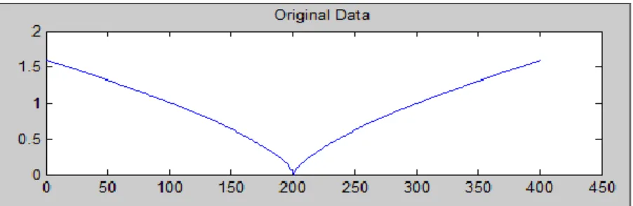
Fig. 1: Plot of data points from the function in Case 1 with no outliers, δ=0.
The data used for this experiment consist of N=400 points that were generated by sampling the independent variable in the range of [-2, 2] with interval 0.01.
Case 2- Another 1-D function to be approximated was as considered in many articles (Chen and Jain, 1994; Cuang et al., 2004; Rusiecki, 2012) defined as:
x x
ysin( ) (2) The data used for this experiment consist of N=1500 points that were generated by sampling the independent variable in the range of [-7.5, 7.5] with interval 0.01.
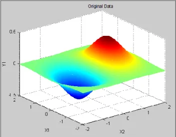
Case 3- The second approximation was as suggested by El-Melegy (2009) and Rusiecki (2012) which can be defined as:
x x e x y
2 2 2 1
Fig. 2: Plot of data points from the function in Case 2 with no outliers, δ=0.
Fig. 3: Plot of data points from the function in Case 3 with no outliers, δ=0.
The data points were created by sampled function on the regular 16 x 16 grid. Here, the data set were generated by sampling the independent variables, x1, x2
[-2, 2] with interval 0.01.Methodology Overview:
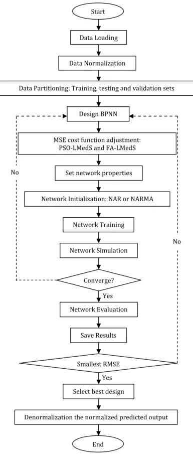
In the research flowchart in Figure 4, the research process can be clearly seen. Here, the existing robust estimators on backpropagation neural network were implemented. To answer the main objective of the study, the possible hybrid robust estimators in nonlinear autoregressive (NAR) and nonlinear autoregressive moving average (NARMA) of neural network time series were done using MATLAB R2012a. At this step, MATLAB scripts or codings were written parallel to the mathematical formulation done earlier. After that, the performance of the proposed robustified neural network models were compared using simulation data; 1-D and 2-D using the standard performance measure, root mean square error (RMSE). Then the robust NAR and BPNN-NARMA method were tested on benchmark data. The comparative results were drawn in those steps.
A. Robust Backpropagation Algorithm:
The most important part of the study is the mathematical formulation improvement part of backpropagation neural network algorithm using statistical robust estimators. To make robust the traditional backpropagation
algorithm based on the M-estimators concept for reducing outlier effect, the squared residuals 2
i
in the network error by another function of the residuals
N
i i
N
E 1 2, (4)
and this yields,
) ( 1
N
i i
N
E , (5)
Ni ji
i i j i j W N W E W , , , ) (
( ). . i, N i j j i O net f r
N
(6)
where α is a user-supplied learning constant, Oh is the output of the ith hidden neuron, Oj=fj(netj) is the output of the jth output neuron, netj=
i i
jiO
W
is the induced local field produced at the input of the activation function associated with the output neuron (j), and fj is the activation function of the neurons in the output layer. In this work, a linear activation function (purelin) will be used in the output layer’s neurons. The weights from the input to hidden neurons Wj,i are updated as
Ni ji
i ji ji W N W E W , ) (
( ). . ,. . i, i i i j N i j j i j I net f W net f r N
(7)where Ii is the input to the ith input neuron, netj= i
i i j O
W
, is induced local field produced at the input of theactivation function associated with the hidden neuron (i), and fj is the activation function of the neurons in the
hidden layer. We have the intention to use the tan-sigmoid function as the activation function for the hidden layer’s neurons because of its flexibility.
The least-median-of-squares (LMedS) method estimates the parameters by solving the nonlinear minimization problem:
2
minmedii
(8)
That is, the estimator must produce the smallest value for the median of squared residuals computed for the entire data set. It appears that this method is very robust to false matches and also to outliers owing to bad localization (Zhang, 1997). Not like the M-estimators, however, the LMedS problem cannot be mitigated to a weighted least-squares problem. It is perhaps not doable to jot down a straightforward formula for the derivative of LMedS estimator. Hence, deterministic algorithms may not be able to function to minimize that estimator. The Monte-Carlo technique (Zhang, 1997; Aarts et al., 2005) has been practised to solve this problem in some non-neural applications. Stochastic algorithms are also identified as the optimization algorithms which use random search to attain a solution. Stochastic algorithms are thus relatively slow, but there is likelihood that it will find the global minimum. One quite popular optimization algorithm applied to minimize an LMedS-based network error is simulated annealing (SA) algorithm. SA is a superb algorithm because it is relatively general and it has the tendency not to get stuck in either the local minimum or maximum (El-Melegy et al, 2009). However, Rusiecki (2012) discovers that iterated LMedS (ILMedS) tends to outperform the SA-LMedS.
B. Particle Swarm Optimization (PSO):
The PSO algorithm is a stochastic optimization algorithm that iteratively looks for solutions in the problem space by aping the biologically-inspired behavior of ‘flying’ simple agents called the swarm particles
1 2
21
*
p
X
*
rand
C
*
g
X
*
rand
C
V
V
id
id
best
id
best
id (9)which modifies the particle’s position, Xid,
,
id id
id X V
X (10)
and the particle updates its velocity and position as follows:
1 2
21* * * *
) (
* )
(updated V previous C p X rand C g X rand
Vid
id best id best id (11)with the updated particle’s position
) ( * ) ( )
(updated X updated V previous
Where Vid = particle velocity, Xid = particle position, pbest = particle’s best fitness so far, gbest = best solution of
the swarm so far, C1= positive constant known as cognition learning rate, C2 = positive constant known as
social learning rate, rand1 and rand2 = the random numbers uniformly distributed between 0 and 1, α = a time
parameter of each particle, β = the interior weight equals to 0.5 (Shinzawa et al., 2007).
Fig. 4: Flowchart of proposed robust BPNN-NAR and BPNN-NARMA.
Data Loading Start
Data Normalization
Data Partitioning: Training, testing and validation sets
Design BPNN
Set network properties
Network Initialization: NAR or NARMA MSE cost function adjustment:
PSO-LMedS and FA-LMedS
Network Training
Network Simulation
Network Evaluation Converge?
Save Results
Select best design Smallest RMSE
End No
No
Yes
Yes
C. Firefly Algorithm:
The FA was developed by Xin-She Yang at Cambridge University in 2007 based on the flashing pattern of tropical fireflies (Yang, 2008; Yang, 2009), and cuckoo search algorithm which was inspired by the brood parasitism of some cuckoo species (Yang and Deb, 2009). In the simplest case for maximum optimization problems, the brightest, I of a firefly for a particular location, x could be chosen as I(x) f(x). However, the attractiveness β is relative and it should be judged by other fireflies, hence it will differ with the distance rij between firefly i and firefly j. In addition, light intensity decreases with the distance from its source, and light is also absorbed by the media, thus the attractiveness is varied with the varying degree of absorption. In the simplest form, the light intensity I(r)varies according to the inverse square law
2 ) ( r I r
I s
(13) where Is is the intensity at the source. For a stated medium with a fixed light absorption coefficient γ, the light intensity I varies with the distance r. That is
r
e I
I 0 (14)
where I0 is the initial light intensity. In order to avoid singularity at r=0 in the expression Is/r2, the combined effect of both the inverse square law and absorption can be approximated as the following Gaussian form
2
0
) (r I e r
I . (15) Since the attractiveness is proportional to the light intensity seen by other fireflies, the attractiveness β of a firefly can be define as
2 0 exp r e (16) where βo is the attractiveness at r=0. Since it is often faster to calculate 1/(1+r2) than an exponential function, the above function can be approximated as
2 0 1 r inv (17) These attractiveness expressions define a characteristic distance Γ=1/γ over which the attractiveness is changing significantly from βo to βoe-1 for the βexp function and βo/2 for the βinv function. In the real time implementation, the attractiveness function β(r) can be monotonically decreasing functions such as the following generalized form
). 1 ( ; )
( 0
m e r rm
(18) For a fixed γ, the characteristic length becomes
). ( ; 1 /
1
m m
On the other hand, for a specific length scale Γ in an optimization problem, the parameter γ can be used as a typical initial value. That is
. 1 m (19) The distance between any two fireflies i and j at xi and xj, respectively is the Cartesian distance,
d k k j k i j i ji x x x x
r 1 2 , , , (20) where xi,k is the kth component of the spatial coordinate xi of ith firefly. In 2-D case, the distance between any two fireflies i and j can be written as
. ) ( )
( 2 2
,j i j i j
i x x y y
r
(21) The movement of a firefly i is attracted to another brighter firefly j is determined by
, ) ( * 2 ,
0 j i i
r i
i x e x x
x ij
(22)
where the second term is due to the attraction and third term is randomization with α being the randomization parameter, and
iis a vector of random numbers being drawn from a Gaussian distribution oruniform distribution. For example, the simplest form is
i can be replaced by rand -1/2 where rand is a random number generator uniformly distributed in [0, 1]. For most implementation, usually βo=1 and]
1
,
0
[
algorithm behaves. In theory,
[
0
,
)
, but in actual practice,
0
(
1
)
is determined by the characteristic length Γ of the system to be optimized. Thus, for most applications, it typically varies from 0.1 to 10 (Yang, 2008; Pal et al., 2012).The descriptive measures for model selection was root mean square error (RMSE) which can be written as
N t RMSE N t
1 2 . (23)
Similar as many previous research efforts demonstrated, it is possible to train the FNNs with median neuron input function with gradient-based algorithms (Rusiecki, 2008). In these networks, simple summation in the neuron input is replaced by the median input function, which also causes non-differentiability if the network error function. The RBP learning algorithm was developed to eliminate the effect of slow convergence for the very low gradient magnitude caused by the flat regions of sigmoid activation functions. This is the reason why the algorithm is more suitable to the LMedS error function, just simply because proper estimation of the sign of the gradient is more likely than proper estimation of its exact value (Rusiecki, 2012). The steps of the approximate RBP algorithm for the LMedS error criteria can be written as follows
Step 1: Use backpropagation to calculate derivatives of the MSE performance function, εmed
Step 2: Update the network weights
Step 3:Modify elements of data with background noise Step 4: Calculate the network LmedS performance εmed
Step 5: If the LMedS performance is minimized to the assumed goal, or the number of epochs exceeds the maximum number of epochs, stop training. Otherwise go to the first step.
The basic NAR-ANN formulation can be represented as below;
( 1), ( 2),..., ( )
exp 1 ) ( , 0 , 1 y i j j m j j n t x t x t x w w w x G
(24)The finalized NARMA-ANN formulation can be represented as below;
t y i j j m j j t n t t t n t x t x t x w w w x G )] ( )] ( ),..., 2 ( ), 1 ( ), ( ),..., 2 ( ), 1 ( [ exp 1 ) ( , 0 , 1 (25)where G(x) is the estimated model, and x(t-1), x(t-2),…, x(t-ny) are lagged output terms. Then, u(t-nk), u(t-nk -1),…u(t-nk-nu) are current and/or lagged input terms, ε(t-1), ε(t-2),…ε(t-nε) are lagged residual terms, and the lagged residual terms are obtained recursively after the initial model (based on the input and output terms) is found. Hence, ε(t) or εt are the white noise residuals. Parameter nk is the input signal time delay.
RESULTS AND DISCUSSIONS
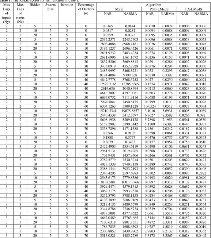
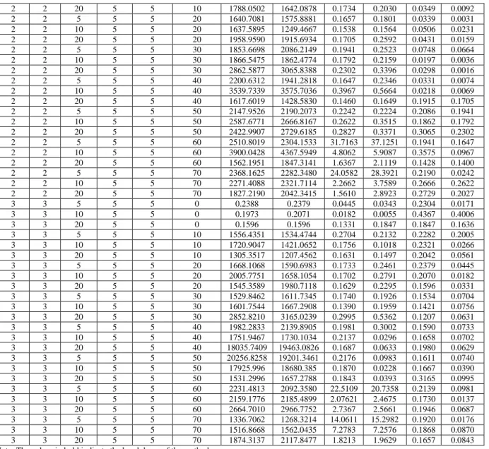
Based on the Tables 1, 2 and 3, the traditional algorithm produced the best results based on the smallest RMSE values for the clean data without outliers. This outcome is parallel with the claim that MSE error function is optimal for the data without outliers by El-Melegy et al. (2009), Rusiecki (2012) and Beliakov et al. (2014).
However, the situation is changed for the data containing artificially generated outliers where the MSE-based method completely loses its efficiency. This can be proven by the breakdowns of the method as shown in Tables 1, 2 and 3. Both robust algorithms of PSO-LMedS and FA-LMedS perform significantly better compared to MSE-based cost function. Moreover, by just comparing the two evolutionary optimization algorithms, FA-LMedS has shown greater performance with the lowest RMSE values in all three cases, as shown in Tables 1, 2 and 3. This is maybe due to the reason that firefly algorithm perform better for higher level of noise (Pal et al., 2012) and when it incorporated into backpropagation neural network training algorithm, it converge at faster rate with minimum feedforward neural network design (Nandy et al., 2012). As mentioned by Yang (2009), the fireflies algorithm is the special case of accelerated particle swarm optimization algorithm. Furthermore, compared to FA-LMedS, the PSO-LMedS algorithm tends to achieve greater RSME as the percentage of outliers increase. In this case, PSO-LMedS was observed to produce greater errors for the data consisting outliers more than 60 percent, as shown in Tables 1, 2 and 3.
Based on the empirical results of this research, there are four general conclusions can be drawn concerning the tested algorithms:
1. The learning algorithm based on the MSE function works best when the data are clean or not corrupted by outliers.
3. The FA-LMedS algorithm seems to outperform the PSO-LMedS for the data with gross errors.
4. The robust NARMA-ANN method performed the best via FA-LMedS compared to the robust NAR-ANN method.
Table 1: The RMSE scores for test function in Case 1. Max
Lags of inputs
(Ny) Max Lags of errors
(Ne)
Hidden Swarm Size
Iteration Percentage of Outliers
(δ)
Algorithm
MSE PSO-LMedS FA-LMedS
NAR NARMA NAR NARMA NAR NARMA
2 2 5 5 5 0 0.0165 0.0144 0.0070 0.0024 0.0006 0.0006
2 2 10 5 5 0 0.0317 0.0232 0.0094 0.0088 0.0009 0.0009
2 2 20 5 5 0 0.0559 0.0373 0.0095 0.0035 0.0010 0.0009
2 2 5 5 5 10 2537.2571 2243.7403 0.0096 0.0088 0.0073 0.0055
2 2 10 5 5 10 7806.4086 6968.4181 0.0076 0.0085 0.0040 0.0048
2 2 20 5 5 10 3197.1237 2696.4526 0.0061 0.0071 0.0024 0.0013
2 2 5 5 5 20 2691.9232 2483.4234 0.0274 0.0128 0.0005 0.0069
2 2 10 5 5 20 2681.6996 1561.1672 0.0236 0.0153 0.0041 0.0073
2 2 20 5 5 20 3837.5206 3669.8813 0.0291 0.0286 0.0092 0.0026
2 2 5 5 5 30 3436.0919 4352.2928 0.0376 0.0294 0.0003 0.0050
2 2 10 5 5 30 3483.9997 3468.8221 0.0321 0.2293 0.0047 0.0056
2 2 20 5 5 30 8194.4084 9399.368 0.0530 0.3392 0.0068 0.0071
2 2 5 5 5 40 4842.7778 3768.5752 0.0271 0.0250 0.0060 0.0024
2 2 10 5 5 40 12529.7165 12785.6565 0.1574 0.0971 0.0042 0.0018
2 2 20 5 5 40 2616.636 2040.8494 0.0213 0.0060 0.0023 0.0020
2 2 5 5 5 50 4613.7007 4797.0081 0.0503 0.0276 0.0028 0.0070
2 2 10 5 5 50 6696.0732 7111.9116 0.0688 0.0193 0.0071 0.0073
2 2 20 5 5 50 5870.884 7450.8175 0.0799 0.011 0.0007 0.0028
2 2 5 5 5 60 6304.1263 5309.1228 10.0524 7.0512 0.0037 0.0034
2 2 10 5 5 60 15210.3341 19075.8857 3.1016 5.6931 0.0005 0.0039
2 2 20 5 5 60 2440.4538 3412.5697 6.7627 8.3582 0.0266 0.092
2 2 5 5 5 70 5608.1938 5209.1128 5.7898 7.1953 0.0561 0.0530
2 2 10 5 5 70 5159.2982 5390.3442 5.1300 3.6382 0.0445 0.0937
2 2 20 5 5 70 3338.7296 4171.1588 2.4361 2.0342 0.0182 0.0149
3 3 5 5 5 0 0.2266 0.9105 0.0598 0.0061 0.0331 0.0381
3 3 10 5 5 0 0.1888 0.5777 0.0476 0.0737 0.0704 0.0363
3 3 20 5 5 0 0.8679 0.3433 0.0177 0.0954 0.0756 0.0610
3 3 5 5 5 10 2422.4903 2354.6119 0.0290 0.0106 0.0631 0.0243
3 3 10 5 5 10 2961.5131 2019.4265 0.0308 0.0471 0.0733 0.0626
3 3 20 5 5 10 1703.9431 1457.9506 0.0266 0.0561 0.0702 0.0752
3 3 5 5 5 20 2782.5779 2530.3214 0.0301 0.0203 0.0629 0.0421
3 3 10 5 5 20 4023.1339 2749.3138 0.0289 0.0742 0.0740 0.0395
3 3 20 5 5 20 2388.1344 3923.2193 0.0265 0.0052 0.0390 0.0408
3 3 5 5 5 30 2340.4295 2597.6883 0.0302 0.0089 0.0995 0.2822
3 3 10 5 5 30 2565.6173 2779.8586 0.0193 0.0020 0.0981 0.0690
3 3 20 5 5 30 8138.588 10017.3766 0.0897 0.0312 0.0137 0.0487
3 3 5 5 5 40 3929.4474 4579.1315 0.0392 0.0628 0.0687 0.0609
3 3 10 5 5 40 3069.3175 2993.2578 0.0456 0.0206 0.0176 0.0983
3 3 20 5 5 40 3252.8795 3788.1158 0.0284 0.0468 0.0870 0.0507
3 3 5 5 5 50 4103.3899 3686.9169 0.0473 0.0135 0.0843 0.0731
3 3 10 5 5 50 3213.4135 3489.5679 0.0349 0.0253 0.0251 0.0554
3 3 20 5 5 50 2344.8786 2746.5734 0.0339 0.0704 0.0076 0.0121
3 3 5 5 5 60 4979.5091 4377.9622 5.0661 3.5519 0.0736 0.0320
3 3 10 5 5 60 4662.0489 47763.665 4.3144 3.4804 0.0452 0.0295
3 3 20 5 5 60 7100.6318 8801.7551 7.4872 6.3311 0.0989 0.0926
3 3 5 5 5 70 1786.7835 1608.6392 19.787 4.5819 0.0020 0.0019
3 3 10 5 5 70 2300.8852 2439.9802 2.9803 8.2132 0.0312 0.0362
3 3 20 5 5 70 3513.0521 4485.2789 3.3173 3.3565 0.0628 0.0402
Note: The values in bold indicate the breakdown of the method
Table 2: The RMSE scores for test function in Case 2. Max
Lags of inputs
(Ny) Max Lags of errors
(Ne)
Hidden Swarm Size
Iteration Percentage of Outliers
(δ)
Algorithm
MSE PSO-LMedS FA-LMedS
NAR NARMA NAR NARMA NAR NARMA
2 2 5 5 5 0 0.1288 0.1202 0.0305 0.0290 0.0297 0.0252
2 2 10 5 5 0 0.1782 0.1824 0.0716 0.0230 0.0392 0.0982
2 2 20 5 5 0 0.2366 0.2595 0.0225 0.0144 0.0456 0.0751
2 2 5 5 5 10 1592.8770 1801.0386 0.1631 0.2421 0.0284 0.0803
2 2 20 5 5 10 1788.0502 1642.0878 0.1734 0.2030 0.0349 0.0092
2 2 5 5 5 20 1640.7081 1575.8881 0.1657 0.1801 0.0339 0.0031
2 2 10 5 5 20 1637.5895 1249.4667 0.1538 0.1564 0.0506 0.0231
2 2 20 5 5 20 1958.9590 1915.6934 0.1705 0.2592 0.0431 0.0159
2 2 5 5 5 30 1853.6698 2086.2149 0.1941 0.2523 0.0748 0.0664
2 2 10 5 5 30 1866.5475 1862.4774 0.1792 0.2159 0.0197 0.0036
2 2 20 5 5 30 2862.5877 3065.8388 0.2302 0.3396 0.0298 0.0016
2 2 5 5 5 40 2200.6312 1941.2818 0.1647 0.2346 0.0331 0.0074
2 2 10 5 5 40 3539.7339 3575.7036 0.3967 0.5664 0.0218 0.0069
2 2 20 5 5 40 1617.6019 1428.5830 0.1460 0.1649 0.1915 0.1705
2 2 5 5 5 50 2147.9526 2190.2073 0.2242 0.2224 0.2086 0.1941
2 2 10 5 5 50 2587.6771 2666.8167 0.2622 0.3515 0.1862 0.1792
2 2 20 5 5 50 2422.9907 2729.6185 0.2827 0.3371 0.3065 0.2302
2 2 5 5 5 60 2510.8019 2304.1533 31.7163 37.1251 0.1941 0.1647
2 2 10 5 5 60 3900.0428 4367.5949 4.8062 5.9087 0.3575 0.0967
2 2 20 5 5 60 1562.1951 1847.3141 1.6367 2.1119 0.1428 0.1400
2 2 5 5 5 70 2368.1625 2282.3480 24.0582 28.3921 0.2190 0.0242
2 2 10 5 5 70 2271.4088 2321.7114 2.2662 3.7589 0.2666 0.2622
2 2 20 5 5 70 1827.2190 2042.3415 1.5610 2.8923 0.2729 0.2027
3 3 5 5 5 0 0.2388 0.2379 0.0445 0.0343 0.2304 0.0171
3 3 10 5 5 0 0.1973 0.2071 0.0182 0.0055 0.4367 0.4006
3 3 20 5 5 0 0.1596 0.1596 0.1331 0.1847 0.1847 0.1636
3 3 5 5 5 10 1556.4351 1534.4744 0.2704 0.2132 0.2282 0.2005
3 3 10 5 5 10 1720.9047 1421.0652 0.1756 0.1018 0.2321 0.0266
3 3 20 5 5 10 1305.3517 1207.4562 0.1631 0.1497 0.2042 0.0561
3 3 5 5 5 20 1668.1068 1590.6983 0.1733 0.2461 0.2379 0.0445
3 3 10 5 5 20 2005.7751 1658.1054 0.1702 0.2791 0.2070 0.0182
3 3 20 5 5 20 1545.3589 1980.7118 0.1629 0.2295 0.1596 0.0331
3 3 5 5 5 30 1529.8462 1611.7345 0.1740 0.1926 0.1534 0.0704
3 3 10 5 5 30 1601.7544 1667.2908 0.1390 0.1959 0.1421 0.0756
3 3 20 5 5 30 2852.8210 3165.0239 0.2995 0.5362 0.1207 0.0631
3 3 5 5 5 40 1982.2833 2139.8905 0.1981 0.3002 0.1590 0.0733
3 3 10 5 5 40 1751.9467 1730.1034 0.2137 0.0296 0.1658 0.0702
3 3 20 5 5 40 18035.7409 19463.0826 0.1687 0.0633 0.1980 0.0629
3 3 5 5 5 50 20256.8258 19201.3461 0.2176 0.0983 0.1611 0.0740
3 3 10 5 5 50 17925.996 18680.385 0.1870 0.0228 0.1667 0.0390
3 3 20 5 5 50 1531.2996 1657.2788 0.1843 0.0393 0.3165 0.0995
3 3 5 5 5 60 2231.4813 2092.3580 22.5109 20.7358 0.2139 0.0981
3 3 10 5 5 60 2159.1776 2185.4899 2.07621 2.4675 0.1730 0.0137
3 3 20 5 5 60 2664.7010 2966.7752 2.7367 2.5661 0.1946 0.0687
3 3 5 5 5 70 1336.7062 1268.3214 14.0611 15.2982 0.1920 0.0176
3 3 10 5 5 70 1516.8668 1562.0435 7.2783 7.2576 0.1868 0.0870
3 3 20 5 5 70 1874.3137 2117.8477 1.8213 1.9629 0.1657 0.0843
Note: The values in bold indicate the breakdown of the method
Table 3: The RMSE scores for test function in Case 3. Max
Lags of inputs
(Ny) Max Lags of errors
(Ne)
Hidden Swarm Size
Iteration Percentage of Outliers
(δ)
Algorithm
MSE PSO-LMedS FA-LMedS
NAR NARMA NAR NARMA NAR NARMA
2 2 5 5 5 0 0.0226 0.0252 0.0267 0.1636 0.0371 0.0224
2 2 10 5 5 0 0.0436 0.0497 0.0434 0.1184 0.0307 0.0244
2 2 20 5 5 0 0.1112 0.1186 0.1061 0.1258 0.0569 0.0672
2 2 5 5 5 10 4359.7566 8641.6380 0.0365 0.1912 0.057 0.0636
2 2 10 5 5 10 1079.2603 1365.1487 0.1014 0.1184 0.0525 0.0466
2 2 20 5 5 10 3988.2749 4121.7564 0.0388 0.1970 0.1150 0.0153
2 2 5 5 5 20 3717.8782 3244.3472 0.0373 0.1933 0.0756 0.0550
2 2 10 5 5 20 3073.1547 2446.1292 0.0295 0.1718 0.2471 0.0209
2 2 20 5 5 20 5694.1254 6723.3495 0.0513 0.1266 0.0424 0.0272
2 2 5 5 5 30 5730.2224 6368.4176 0.0763 0.1763 0.0517 0.0494
2 2 10 5 5 30 5256.0255 4664.3883 0.0566 0.1381 0.1019 0.0236
2 2 20 5 5 30 11503.8636 11533.4735 0.0884 0.1974 0.0969 0.0136
2 2 5 5 5 40 7562.8682 5504.5465 0.0484 0.1201 0.1372 0.0378
2 2 10 5 5 40 2471.0467 3209.0136 0.2715 0.1211 0.1727 0.0490
2 2 20 5 5 40 4243.4113 2721.2212 0.0432 0.1080 0.0336 0.0046
2 2 5 5 5 50 5179.6874 4948.2608 0.0480 0.1191 0.0696 0.0075
2 2 10 5 5 50 10196.5565 12361.8442 0.1195 0.1456 0.0269 0.0201
2 2 20 5 5 50 9697.4329 11364.5493 0.1076 0.1280 0.0248 0.0174
2 2 5 5 5 60 13726.6642 13780.5056 13.8992 17.2684 0.0156 0.0136
2 2 10 5 5 60 1727.7562 3490.8264 2.6921 1.1894 0.0366 0.0290
2 2 5 5 5 70 7393.3438 8065.0819 62.3462 49.6728 0.0346 0.0321
2 2 10 5 5 70 9217.7368 14128.0656 10.0843 11.7510 0.0939 0.0530
2 2 20 5 5 70 5306.5654 8367.3694 3.3467 8.2714 0.0376 0.0271
3 3 5 5 5 0 0.0937 0.1255 0.0923 0.1138 0.1278 0.1174
3 3 10 5 5 0 0.0749 0.0933 0.1088 0.0298 0.0204 0.0113
3 3 20 5 5 0 0.0381 0.0379 0.0247 0.0574 0.0479 0.0102
3 3 5 5 5 10 3636.3138 4549.1711 0.0391 0.0977 0.0711 0.0287
3 3 10 5 5 10 6106.0489 4076.2713 0.0501 0.0239 0.0745 0.0399
3 3 20 5 5 10 2437.9512 2242.0911 0.0277 0.0664 0.1014 0.0085
3 3 5 5 5 20 6265.6872 6059.5287 0.0558 0.0362 0.0388 0.0097
3 3 10 5 5 20 7522.1978 7795.0577 0.0760 0.0757 0.0373 0.0028
3 3 20 5 5 20 4214.6130 5269.1885 0.0488 0.0192 0.0295 0.0053
3 3 5 5 5 30 3956.8955 3710.3527 0.0639 0.0528 0.0513 0.0086
3 3 10 5 5 30 4083.2797 3841.2332 0.0315 0.1776 0.0763 0.0303
3 3 20 5 5 30 2822.7018 2875.1272 0.1944 0.1409 0.0566 0.0292
3 3 5 5 5 40 6906.748 9012.3312 0.0985 0.1139 0.0884 0.0391
3 3 10 5 5 40 4870.0912 5275.4700 0.0578 0.2405 0.0484 0.0050
3 3 20 5 5 40 6093.7314 6934.9149 0.0500 0.2238 0.2715 0.0970
3 3 5 5 5 50 9831.8046 8903.4344 0.1178 0.3432 0.0432 0.0059
3 3 10 5 5 50 5076.8150 4965.6695 0.0694 0.0635 0.0480 0.0275
3 3 20 5 5 50 7313.6695 5727.4593 0.0803 0.0834 0.1195 0.0193
3 3 5 5 5 60 55470.641 7144.9387 8.7385 9.5403 0.1076 0.0114
3 3 10 5 5 60 11215.7927 12026.7402 9.4028 6.6874 0.1389 0.0704
3 3 20 5 5 60 13201.5013 12719.1829 1.7246 1.5251 0.2692 0.0156
3 3 5 5 5 70 2128.2096 2340.6143 22.445 14.9818 0.0410 0.0835
3 3 10 5 5 70 3316.8333 3011.2852 4.1315 2.0322 0.0623 0.0719
3 3 20 5 5 70 5455.9473 8776.2548 6.2097 2.4918 0.1008 0.0036
Note: The values in bold indicate the breakdown of the method.
Conclusions and Recommendations:
In this paper we presented novel robust backpropagation neural network learning algorithm based on the hybrid firefly algorithm with least median of squares, also known as FA-LMedS. Our algorithm is not only robust to the presence of various amounts of outliers but also faster and more accurate compared to the other methods, such as M-estimators, ILMedS, PSO-LMedS known from the previous works. The performance superiority of our method in comparison to other algorithms, in the presence of different degree of outliers, was empirically demonstrated.
For the clean data or the data which do not suffer from outliers problem, the conventional backpropagation based on the MSE algorithm performed the best. Moreover, for data consisting outliers more than 50 percent, it can be concluded that the model built by the network trained with the FA-LMedS learning algorithm is more precise than for the traditional method as well the modern ones such as ILMedS and PSO-LMedS, in the case of data contaminated with gross errors and outliers. This new proposed robust stochastic algorithm based on the LMedS estimator has demonstrated even improved robustness over the other estimators whereby it managed to tolerate up to 70 percent outliers while maintaining an accurate model on both simulation and real data.
The proposed robust algorithms for training neural networks can also be used in applications other than function approximation and system identification, such as pattern recognition, system identification, machine learning, artificial intelligence, financial risk management, robotic, as well as quality control and optimization. In future efforts, several alternatives shall be taken into consideration in this research, which are:
i) To increase the number of iteration and swarm size particle for both PSO-LMedS and FA-LMedS and compare their performances.
ii) To find faster and more proficient alternatives to minimize the LMedS error criterion function, e.g. by manipulating the enhanced versions of the RBP method.
iii) To apply other faster training algorithm into the network and further compare the results, such as traincgf (El-Melegy et al., 2009), trainrp (Rusiecki, 2014) and trainlm (Beliakov et al., 2012).
iv) To apply other existing statistical robust stochastic estimators and soon hybrid them with fast deterministic algorithms.
v) To train the network using different activation functions as mentioned by Sibi et al. (2013).
vi) To further improve the backpropagation learning algorithm using improved version of least trimmed squares (LTS) such those as proposed by Beliakov et al. (2012), Alfons et al. (2013) and Zioutas et al. (2007). vii) To test the PSO-LMedS and new FA-LMedS algorithm on approximation task of a 2-D spiral as suggested by Rusiecki (2012), as well as Data set 4 to Data set 14 as suggested by Beliakov et al. (2012).
viii)To compare the average time performance (in seconds) for all the tested algorithms in simulation studies as shown by Rusiecki (2012).
x) To further hybrid neural network with improved version firefly algorithm such the one proposed by Abdullah et al. (2012), called Hybrid Evolutionary Firefly Algorithm (HEFA).
ACKNOWLEDGEMENT
We would like to dedicate our appreciation and gratitude to Unit Kerjasama Awam Swasta (UKAS) of Prime Minister’s Department, Construction Industry Development Board (CIDB) and Malaysian Statistics Department. Special thanks also go to Kulliyyah of Science, International Islamic University Malaysia for supporting this research under the IIUM Research Funding, as well as Ministry of Higher Education (MOHE) for scholarship given to Mr. Saadi.
REFERENCES
Abdullah, A., S. Deris, M.S. Mohamad and S.Z.M. Hashim, 2012. A new hybrid firefly algorithm for complex and nonlinear problem. In Distributed Computing and Artificial Intelligence, 673-680.
Alfons, A., C. Croux and S. Gelper, 2013. Sparse least trimmed squares regression for analyzing high-dimensional large data sets. The Annals of Applied Statistics, 7(1): 226-248.
Beliakov, G., A. Kelarev and J. Yearwood, 2012. Derivative-free optimization and neural networks for robust regression. Optimization, 61(12): 1467-1490.
Box, G.E., G.M. Jenkins and G.C. Reinsel, 1994. Time series analysis, forecasting and control, Ed. Prentice Hall.
Brajevic, I. and M. Tuba, 2013. Training Feed-Forward Neural Networks Using Firefly Algorithm. Recent Advances in Knowledge Engineering and Systems Science, 156-161.
Chen, D.S. and R.C. Jain, 1994. A robust back propagation learning algorithm for function approximation. IEEE Trans. Neural Networks, 5(3): 467-479.
Chuang, C., J.T. Jeng and P.T. Lin, 2004. Annealing robust radial basis function networks for function approximation with outliers. Neurocomputing, 56: 123-139.
Chuang, Su, S. and C. Hsiao, 2000. The annealing robust backpropagation (ARBP) learning algorithm. IEEE Trans Neural Networks, 11(5): 1067-1076.
Connor, J.T. and R.D. Martin, 1994. Recurrent neural networks and robust time series prediction. IEEE Transactions of Neural Networks, 5(2): 240-253.
David, S.V.A., 1995. Robustization of a learning method for RBF networks. Neurocomputing, 9(1): 85-94. El-Melegy, M.T., M.H. Essai and A.A. Ali, 2009. Robust training of artificial feedforward neural networks. Found Comput Intell 1, Springer, Berlin, Heidelberg, 1: 217-242.
Engelbrecht, A.P., 2007. Computational intelligence: an introduction. Wiley. com.
Franses, P.H. and K.V. Griensven, 1998. Forecasting exchange rates using neural networks for technical trading Rules. Studies in Nonlinear Dynamics and Econometrics, 4(2): 109-114.
Gabr, M.M., 1998. Robust estimation of bilinear time series models. Comm. Statist, Theory and Meth, 27(1): 41-53.
Gitman, L.J. and C. McDaniel, 2008. The future of business, The essentials, South-Western Pub.
Hampel, F.R., E.M. Ronchetti, P.J. Rousseeuw and W.A. Stahel, 1986. Robust Statistics, The approach based on influence functions. Wiley, New York.
Hector, Claudio, M. and S. Rodrigo, 2002. Robust Estimator for the Learning Process in Neural Network Applied in Time Series. Artificial Neural Networks-ICANN 2002, Springer Berlin Heidelberg, 1080-1086.
Huber, P.J., 1981. Robust Statistics. John Wiley and Sons, New York.
Jing, X., 2012. Robust adaptive learning of feedforward neural networks via LMI optimizations. Neural Networks, 31: 33-45.
Kaastra and M.S. Boyd, 1995. Forecasting futures trading volume using neural networks. The Journal of Futures Markets, 18: 953-970.
Kamaruddin, S.B.A., N.A.M. Ghani and N.M. Ramli, 2013. Determining the Best Forecasting Method to Estimate Unitary Charges Price Indexes of PFI Data in Central Region Peninsular Malaysia. AIP Conf. Proc., 1(1522): 1232-1239.
Kamaruddin, S.B.A., N.A.M. Ghani and N.M. Ramli, 2014. Best Forecasting Models for Private Financial Initiative Unitary Charges Data of East Coast and Southern Regions in Peninsular Malaysia. International Journal of Economics and Statistics, 2: 119-127.
Liano, K., 1996. Robust error measure for supervised neural network learning with outliers. IEEE Trans. Neural Networks, 7(1): 246-250.
Pal, S.K., C.S. Rai and A.P. Singh, 2012. Comparative Study of Firefly Algorithm and Particle Swarm Optimization for Noisy Non-Linear Optimization Problems. International Journal of Intelligent Systems and Applications, 10: 50-57.
Pearson, R.K., 2002. Outliers in process modeling and identification. Control Systems Technology, IEEE Transactions on, 10(1): 55-63.
Pei, L., S.H. Chen, H.H. Yang, C.T. Hung and M.R. Tsai, 2008. Application of artificial neural network and SARIMA in portland cement supply chain to forecast demand. Natural Computation, 3: 97-101.
Pernia-Espinoza, V., J.B. Ordieres-Mere, F.J. Martinez-de-Pison and Gonzalez-Marcos, 2005. A TAO-robust backpropagation learning algorithm. Neural Network, 18(2): 191-204.
Rakitianskaia, A.S. and A.P. Engelbrecht, 2012. Training feedforward neural networks with dynamic particle swarm optimisation. Swarm Intelligence, 6(3): 233-270.
Rousseeuw, P.J. and A.M. Leroy, 1987. Robust regression and outlier detection, Wiley, New York.
Rusiecki, A., 2012. Robust Learning Algorithm Based on Iterative Least Median of Squares. Neural Process Lett., 36: 145-160.
Rusiecki, A., 2008. Robust MCD-based backpropagation learning algorithm. In Artificial Intelligence and Soft Computing-ICAISC 2008, Springer Berlin Heidelberg, 154-163.
Rusiecki, A.L., 2005. Fault tolerant feedforward neural network with median neuron input function. Electronics Letters, 41(10): 603-605.
Shinzawa, H., J.H. Jiang, M. Iwahashi and Y. Ozaki, 2007. Robust curve fitting method for optical spectra by least median squares (LMedS) estimator with particle swarm optimization (PSO). Analytical sciences, 23: 781-785.
Sibi, P., S.A. Jones and P. Siddarth, 2013. Analysis Of Different Activation Functions Using Back Propagation Neural Networks. Journal Of Theoretical And Applied Information Technology, 47(3): 1264-1268.
Sun, S. and F. Jin, 2011. Robust co-training. International Journal of Pattern Recognition Artificial Intelligence, 25(7): 1113-1126.
Yang, X.S., 2008. Nature-Inspired Metaheuristic Algorithms. Luniver Press, UK.
Yang, X.S., 2009. Firefly Algorithms for Multimodal Optimization. Proceeding of the 5th Symposium on Stochastic Algorithms, Foundations and Applications, (Eds. O. Watanabe and T. Zeugmann), Lecture Notes in Computer Science, 5792: 169-178.
Yang, X.S. and S. Deb, 2009. Cuckoo Search via Levy Flights. Proceedings of World Congress on Nature & Biologically Inspired Computing (NaBIC 2009, India), IEEE Publications, USA, 210-214.
Yang, X.S., 2008. Nature-Inspired Metaheuristic Algorithms, Luniver Press, UK.
Yang, X.S., 2009. Firefly Algorithms for Multimodal Optimization. Proceeding of the 5th Symposium on Stochastic Algorithms, Foundations and Applications, (Eds. O. Watanabe and T. Zeugmann), Lecture Notes in Computer Science, 5792: 169-178.
Yang, X.S., 2009. Firefly algorithms for multimodal optimization. In Stochastic algorithms: foundations and applications, 169-178.
Yang, X.S. and S. Deb, 2009. Cuckoo Search via Levy Flights. Proceedings of World Congress on Nature & Biologically Inspired Computing, 210-214.
Yang, X.S. and X. He, 2013. Firefly Algorithm: Recent Advances and Applications. International Journal Swarm Intelligence, 1(1): 36-50.
Yang, X.S., 2010a. Engineering Optimization: An Introduction with Metaheuristic Applications. John Wiley and Sons, USA.
Yang, X.S., 2010b. A New Metaheuristic Bat-inspired algorithm. Nature Inspired Cooperative Strategies for Optimization (NICSO 2010), (Eds. J. R. Gonzales et al.), Springer, SCI, 284: 65-74.
Zhang, Z., 1997. Parameter estimation techniques: A tutorial with application to conic fitting. Image and Vision Computing Journal, 15(1): 59-76.