To Cite This Article: Sumana B.V and T. Santhanam., Optimizing K-means in Cascading Clustering and Classification. Aust. J. Basic & Appl. Sci., 10(9): 184-206, 2016

(1)

AUSTRALIAN JOURNAL OF BASIC AND

APPLIED SCIENCES

ISSN:1991-8178 EISSN: 2309-8414 Journal home page: www.ajbasweb.com

Open Access Journal

Published BY AENSI Publication

This work is licensed under the Creative Commons Attribution International License (CC BY). http://creativecommons.org/licenses/by/4.0/

To Cite This Article: Sumana B.V and T. Santhanam., Optimizing K-means in Cascading Clustering and Classification. Aust. J. Basic & Appl. Sci., 10(9): 184-206, 2016

Optimizing K-means in Cascading Clustering and Classification

1_{Sumana B.V and}2_{T. Santhanam}

1_{Assistant Professor, Department of Computer Science, Vijaya College, Jayanagar, Bangalore - 560011, India.} 2

Associate Professor and Head, PG and Research Department of Computer Science and Applications, D. G. Vaishnav College, Chennai - 600106, India.

Address For Correspondence:

Sumana B V., Assistant Professor Department of Computer Science, Vijaya College, Jayanagar, Bangalore - 560011, India E-mail: [email protected]

A R T I C L E I N F O A B S T R A C T Article history:

Received 3 March 2016 Accepted 2 May 2016 published 26 May 2016

Keywords:

Classification, Clustering, Hybrid, PCA, Boxplot, K-means

Background: Classification is a data mining technique which has been popularly applied for many prediction problems. Recent researches have integrated clustering and classification for prediction problems. Among that, K-means is one of the most commonly used clustering algorithm due to its low computational time, less complexity, termination at local minima and easy implementation. Despite few researchers noticed few factors affecting the performance of K-means algorithm. Objective: To overcome this problem a Hybrid Model with two phases of preprocessing is proposed. The objective of the proposed model is 3 fold 1) to overcome each factor affecting the performance of K-means 2) to increase the performance of the classifier when compared to the other existing models and 3) to reduce the Type II error of the classifier, False negative rate which means that the patients who actually have disease but predicted as not to have disease as in reality it is a very serious problem. Results: The efficiency of the proposed model was evaluated in 2 stages. Stage1, clustering efficiency of K-means was evaluated using Silhouette Index and Rand Index and Stage2, the classifier efficiency was evaluated using confusion matrix with performance measures like accuracy, kappa, ROC, precision, NPV, sensitivity, specificity, Type I, Type II error, FDR, FOR and time to build the model. Results proved that proposed model is more efficient than the existing models in the literature. The performance of the base classifier is maximized such that there is no scope for the ensemble model. All the classifiers on all datasets showed accuracy above 99%. Conclusion: The proposed Hybrid model with preprocessing before K-means improves the performance of the K-means which in turn enhances the classifier performance

INTRODUCTION

(2)

developed which can be applied to any data mining problem (Sumana et al., 2015). It is a very crucial job to choose appropriate technique suitable for a data mining problem.

Since the real world data accumulated in the society is always high dimensional feature space inconsistent with redundant or irrelevant attributes and incomplete or noisy instances etc., presence of these attributes and instances will degrade the classification accuracy. Therefore removal of these attributes and instances is very important as Quality decisions can be made only on good quality data. Therefore pre-processing plays a very important role in removing such attributes and instances because quality of mining depends on the quality of pre-processing which includes data cleaning, data integration, data transformation and data reduction. Data cleaning handles missing values, outliers, noisy data and inconsistent data. Data integration integrates multiple databases or files. Data transformation is a process which converts data from one format to another suitable for mining. Data reduction is a process in which irrelevant, redundant attributes or instances are detected and removed

In recent years hybridization of clustering and classification has been proved to be more efficient than individual classification or clustering in which clustering algorithm is used as a pre-processing algorithm to remove noisy instances (Sumana et al., 2014, Karegowda et al., 2012, Sumana et al., 2015). In the literature there are several papers proposing different clustering algorithm for different data sets like Entropy weighted K-means, fuzzy K-K-means, C-K-means, Entropy Fuzzy K-K-means, DBscan, Cobweb, EM, Make Density Based Cluster etc.,. It is very difficult job to choose an appropriate clustering algorithm for a particular data set. Among several clustering algorithms K-means is most popularly and widely used because of its low computational time, less complexity termination at local minima and can be easily implemented (Sumana et al., 2014, Karegowda et

al., 2012).

Literature Review:

Recent researches have proved that hybridization of clustering and classification improves the classifier accuracy and has been applied by many researchers in almost all domains. Sumana et al (2014) compared the different classification models and proposed a hybrid model combining Classification and clustering using K-means with hybrid feature selection and proved that hybrid model gave good accuracy when compared with other models. Asha Karegowda et al (2012) proposed hybrid model for classification using K-means as a preprocessing algorithm to eliminate wrongly clustered instances then tested the accuracy using Knn classifier. Sumana B.V et al (2014) proposed a hybrid model with CFS feature selection and proved that preprocessing improves k-means which in turn improves classifier accuracy. Pavel etal (2015) has discussed and proved the importance of preprocessing in improving the k-means algorithm. Anusuya et al (2011) has proved that PCA improves the efficiency of k-means. Saranya et al (2013) has proved that normalization improves the performance of k-means. R.S. Somasundaram et al (2011) has discussed the various methods to handle missing values. Minakshi et al (2014) has proved that Knn imputation method is a better way to treat missing values than mean, mode and litwise deletion method. Sumana et al (2015) has proposed hybrid model with K-means and CFS feature selection to enhance both stable and unstable algorithms.

Background Problem:

Though, previous researches have proved that hybridization of clustering and classification improves the classifier accuracy. In the literature there is no paper suggesting the best clustering algorithm suitable for all the datasets. Researchers are getting confused in selecting the clustering algorithm for preprocessing. This research gap has motivated us to propose this model. Among the clustering algorithm K-means is the most widely used clustering algorithm in hybrid clustering and classification model (Sumana et al., 2014, Karegowda et al., 2012, Pavel et al., 2015, Sindhupriya.R, et al., 2014 Prabha. K et al., 2014) despite in the literature there are some papers discussing about the issues that affect the performance of K-means algorithm. K-means has some drawbacks due to which its efficiency is reduced. They are listed as follows 1) K-means does not work efficiently for high dimensional data (Sindhupriya. R et al., 2014) 2) no of clusters to be produced should be specified in advance 3) unable to handle noisy data and outliers and presence of which degrades the performance of K-means 4) cannot be applied directly to categorical data 5) sensitive to initialization of centroids as different centroids produce different clusters (Prabha. K. et al., 2014) 6) sometimes K-means algorithm generates empty clusters where no data points are assigned (Pavel et al., 2015).

(3)

MATERIALS AND METHODS

The proposed model is evaluated using R language on Pima Indian Diabetes, Breast Cancer dataset and Liver datasets collected from UCI Machine Learning Repository using stratified 10-fold cross validation to test the accuracy and time complexity of the classifiers. In the following subsections the dataset used, experimental setup of the proposed model and results are discussed. The impacts of how classifier accuracy is increased with pre-process and removal of outliers before K-means is examined.

In hybrid model efficiency of a classifier is improved by the clustering algorithm. Hence it is very important to improve the efficiency of clustering algorithm. Usually data accumulated in this Real world will have noisy data, errors, inconsistencies, outliers and lack of variable values. Quality data gives quality results therefore pre-processing is an important step before clustering. The objective of this work is twofold 1) to provide a unique clustering algorithm suitable for all the datasets and 2) to reduce the Type1 error of the classifier which is, false positive rate means the patients who actually does not have disease but predicted as to have disease. Therefore a model is proposed in this paper in which the most popularly used K-means is used as a clustering algorithm. To improve the efficiency of K-means its drawbacks are studied well and each drawback is treated with a pre-processing step.

Proposed model:

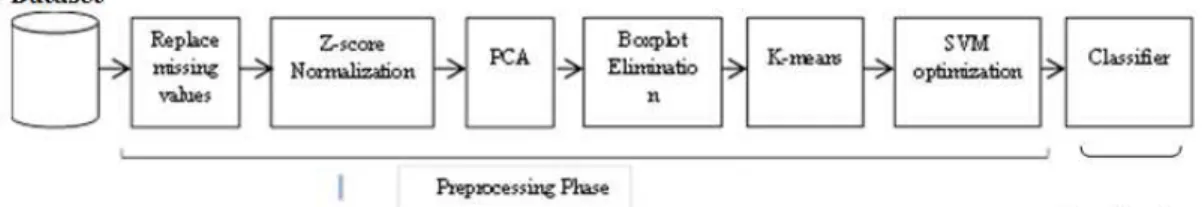
The proposed model is developed in 2 phases; 2 stage pre-process phase and classification phase. Initially in the first stage of pre-processing the datasets selected from the UCI repository is cleaned by filling all the instances with missing values followed by normalization using Z-score, as the attribute values are of different scales further followed by feature extraction using PCA and in the second stage of pre-processing outliers are removed using Boxplot to improve the quality of clustering algorithm and then K-means clustering algorithm is applied to remove the incorrectly clustered samples which is further optimized using SVM to remove the misclassified instances which were wrongly clustered by K-means algorithm. Finally the correctly clustered samples from the previous phase were trained using 9 classifiers to build the final classifier model using stratified 10 fold cross validation.

Fig. 1: Block diagram of the proposed model

Preprocessing Phase:

In the literature few standard procedures about preprocessing is explained (Pavel et al., 2015) which involves steps like data cleaning to handle missing values, data integration to integrate data from different databases, data transformation includes normalization means data are scaled to common scale ranging between 0.0 to 1.0 to avoid higher range values dominating in the analysis and data reduction to obtain reduced representation without losing any information. Data reduction is achieved using feature selection or feature extraction. Feature extraction is more effective when compared to feature selection because it combines correlated attributes and creates new ones which are superior to original attributes whereas feature selection evaluates the quality of attributes and selects the best set. In the proposed PCA is used for feature extraction.

Treating missing Values:

(4)

Normalization:

Normalization is an important preprocessing step in Data Mining which transforms the input values of all attributes into a common scale to avoid attributes having greater numeric values dominating the smaller numeric range values. Doing so, it gives equal importance to all the variables. Min-max normalization, Z-Score normalization and Decimal Scaling normalization are the various types of normalization techniques available in the literature (Saranya. C et al., 2013) A standard normal distribution is a normal distribution with zero mean and unit variance, Z-scores also called as Zero mean normalization is the most commonly used method which converts all attribute values with an average of 0 and variance of 1. This is adapted in the proposed model before performing PCA and K-means because to provide equal weight for all attributes while calculating the principal components and generating clusters. Since Euclidean distance is used for calculating centroids the clusters generation will be strongly influenced by the magnitudes of the outliers. To overcome this data is normalized. Normalizing the data not only generate good quality clusters it will also speed up the learning phase of the classifier.

Principal Component Analysis:

Principal component analysis (PCA) is a popularly known data preprocessing technique used for dimensionality reduction that generates principal components which are linear combination of the original data. These principal components are orthogonal and uncorrelated to each other explaining the variation in the data. The principal components with higher variance have higher weightage than the principal component with lower variance hence normalizing the data to a common scale before PCA is important. If d dimensional dataset is considered excluding the class variable, compute the covariance or correlation matrix of the dimensions Find eigenvectors and eigenvalues from the covariance or correlation matrix. Sort eigenvectors in decreasing order of eigenvalues and choose k eigenvectors with the largest eigenvalues to form a d x k dimensional matrix and transform on to a new subspace called principal components. The principal components are linear combinations of the original variables explaining the variance in orthogonal dimensions. The first principal component explains the largest variability in the data as possible, and each succeeding component explains next highest variance. This continues until it is equal to the original number of variables. The PCs with high variability are selected neglecting the PCs with less variability thus dimensionality reduction is achieved.

Principal component analysis (PCA) is a most widely used feature extraction method for linear datasets adapted in the proposed model for 3 reasons 1) to transform higher dimensional data into a lower dimensional data as it is easier to visualize the data when reduced to lower dimensions (Xu, Qin et al., 2015, Janecek Andreas GK et al., 2008) 2) to transform correlated variables into a set of linear combinations of the original data called principal components which are uncorrelated with each other because presence of correlated variables degrades the prediction accuracy (Howley et al., 2006).

Outlier elimination:

Outliers are observations present in the data which are different from all other observations in the data. Clustering algorithms use distance metrics to calculate centroids of the clusters. Presence of outliers deviate the cluster centroid and degrades the performance of clustering algorithms. To overcome this, a research direction is suggested in (Pavel et al., 2015, Vaishali R. Patel., et al., 2011, Ville Hautam aki et al., 2005) to remove outliers before performing K-means clustering. Hence Boxplot technique is adapted in this proposed model for the removal of outliers.

K-means Clustering:

K- Means is a well-known partition algorithm which groups the data into k clusters in which the resulting objects of one cluster are similar in the same cluster and dissimilar to that of other cluster using the following steps

1. Takes k as an input to cluster into k groups. 2. Randomly select k points as the initial centroids.

3. Calculate the distance between each point and cluster centers. 4. Assign all data points to the closest centroid.

5. Recalculate the new centroid of each cluster using the distance formula

4. Repeat steps 3 and 5 until a reassignment stops.

Optimizing K-means with SVM:

(5)

define the hyper plane. An optimal separating hyper plane is the hyper plane that maximizes the margin. To classify the data SVMs first find the maximal margin which separates two classes and then outputs the hyper plane separator at the center of the margin. New data is classified by determining on which side of the hyper plane it belongs and hence to which class it should be assigned.

The goal of classification is to minimize the test error therefore classification methods are also used for optimization problems. To enhance the prediction accuracy of the classifier clustering algorithms are used as a preprocessing algorithm similarly classifiers are used to validate the results produced by clustering algorithms. In this proposed model SVM is used as an optimization algorithm to remove the instances which are wrongly clustered by the clustering algorithm so as to reduce the error of the clustering algorithm. SVM, a binary classifier is adapted in this proposed because the datasets considered are binary classification problem.

Classification:

Finally, the relevant instances identified from the preprocessing phase were trained by 9 different classifiers, one from each type of classifiers of WEKA3.7.2 using stratified 10 fold cross validation. The performances of the classifiers were evaluated based on the confusion matrix. Table 3 illustrates the defined process.

Data set description:

Table 1: Data sets Description

Data Sets No. of Attributes

including class

No of

Classes No. of Instances Missing Values

Diabetes 9 2 768 Yes

Wiscosin Breast cancer 10 2 699 Yes

Bupa liver disorder 7 2 345 No

Estimations for model performance: Stratified 10 fold cross validation method:

In this study stratified Cross Validation with 10 folds has been used for evaluating the classifier models. Cross Validation is a statistical technique used for evaluating the performance of the predictive model and also used to compare learning algorithms by dividing data into 2 segments one used to train a model and the other used to validate the model. Stratification is a process of partitioning the data such that each class is properly represented in both training and test sets. In a stratified 10-fold Cross-Validation the data is divided randomly into 10 parts in which the class is represented in approximately the same proportions as in the full dataset. Each part is held out in turn and the learning scheme trained on the remaining nine-tenths; then its error rate is calculated on the holdout set. The learning procedure is executed a total of 10 times on different training sets, and finally the 10 error rates are averaged to yield an overall error estimate. When seeking an accurate error estimate, it is standard procedure to repeat the CV process 10 times (Sumana et al., 2014).

Performance Measures:

Machine Learning (ML) has several ways of evaluating the performance of the classifiers and clustering algorithms.

Performance measures of clustering algorithms:

Performances of clustering algorithms are evaluated using external cluster validation measure and internal cluster validation measure. External validation measures the quality of the clustering algorithm based on the available information about data sets and the internal validation measures the quality of the clustering algorithm with the data set itself. The commonly used external validation measures are F-measure, Normalized Mutual Information (the average mutual information between every pair of clusters and their class), Rand Index etc., and the commonly used internal validation measures are Davies-Bouldin index, Silhouette index, Dunn index, Partition Coefficient, Entropy, Separation Index, Xie and Beni's Index etc. (Angel Latha Mary S et al., 2015). In this paper Silhouette Coefficient and Rand Index are used for cluster validation.

Silhouette Coefficient is a measure to evaluate the quality of the clustering. The silhouette value measures how similar each point is to other points in the same cluster. The silhouette value for the ith point, Si, is defined as Si = (bi - a i )/ max( a i , bi) where a i is the average distance from the ith point to the other points in the same

cluster as i, and bi is the minimum average distance from the ith point to points in a different cluster, minimized over clusters. It ranges from -1 to +1. A value nearing to 1 specifies that it is well clustered; a value near to 0 specifies that instances are placed between 2 clusters and negative value specifies that the instances are placed in wrong cluster

(6)

clustering which ranges between 0.0 to 1.0, where 0 indicating that the two data clusters do not agree on any pair of points and 1 indicating that the data clusters are exactly the same.

Table 2: Table for calculation of Rand index

Reality

Positive Negative

Ptediction Positive True Positive (TP) False Positive (FP)

Negative False Negative(FN) True Negative (TN)

Rand Index = (TP+TN)/ (TP+FP+TN+FN)

Performance measures of Classification algorithms:

Measures of the quality of classification algorithms are based on the confusion matrix [19] which records correctly and incorrectly recognized examples for each class. Table 3 presents a confusion matrix for binary classification, where TP are True Positive TN is True Negative, FP is False Positive, FN are False Negative. The different measures used with the confusion matrix are:

Table 3: Confusion matrix

Predicted Class

Test Negative(T-) Test Positive(T+)

Actual Class Disease Absent (D-) True Negative (TN) False Positive (FP)

Disease Present (D+) False Negative(FN) True Positive (TP)

Accuracy:

The accuracy of a classifier is the percentage of the test set tuples that are correctly classified by the classifier.

Accuracy = (TP + TN)/(TP + TN + FP + FN)

Kappa:

Kappa is a statistical measure of agreement between the predicted class values to the actual class values. A Kappa value lies between a -1 to 1 scale. A kappa of 1 indicates perfect agreement, whereas a kappa of 0 indicates agreement equivalent to chance and negative values indicate agreement less than chance. Kappa value is calculated using the following formula K = [P (A) – P (E)]/{1 – P (E)] where P(A) is the percentage of agreement between the classifier and the underlying truth calculated. P (E) is the chance of agreement calculated.

ROC:

Receiver operating characteristic (ROC) or ROC curve is a graphical plot used to visualize the performance of a binary classifier. In a ROC curve the true positive rate (Sensitivity) is plotted on the y axis and the false positive rate (100-Specificity) plotted on X axis for different cut-off points. The value nearing to 1 means the model is better.

Time:

The amount of time required to build the model.

Sensitivity:

Sensitivity also known as True positive rate is the percentage of the positive tuples that are correctly classified by the classifier.

TPR= TP/ (TP + FN)

Specificity:

Specificity also known as True negative rate is the percentage of the negative tuples that are correctly classified by the classifier.

TNR= TN/ (TN + FP)

Precision:

Precision also known as positive predictive values PPV is the proportion of the predicted positive cases that were correct

PPV= TP/ (TP + FP)

Negative predictive Value:

(7)

NPV= TN/ (TN + FN)

False positive rate:

The false positive (FP) rate also known as Type I error is the proportion of negative cases that were incorrectly classified as positive

FPR= FP/ (FP+TN)

False negative rate:

The false negative (FN) rate also known as Type II error is the proportion of positive cases that were incorrectly classified as negative

FNR= FN/ (FN+TP)

False Discovery rate:

FDR measures the proportion of discoveries that are false among all discoveries, i.e., the chance of not having the condition among those that test positive

FDR=1-PPV

False Omission rate:

FOR measures the proportion of false negatives which are incorrectly rejected, i.e., the chance of having the condition among those that test negative

FOR=1-NPV

Experimental Results: Preprocessing Phase:

Results after replacing missing values by Prediction method using Weighted Knn from DMwR package and Rpart from rpart package in R

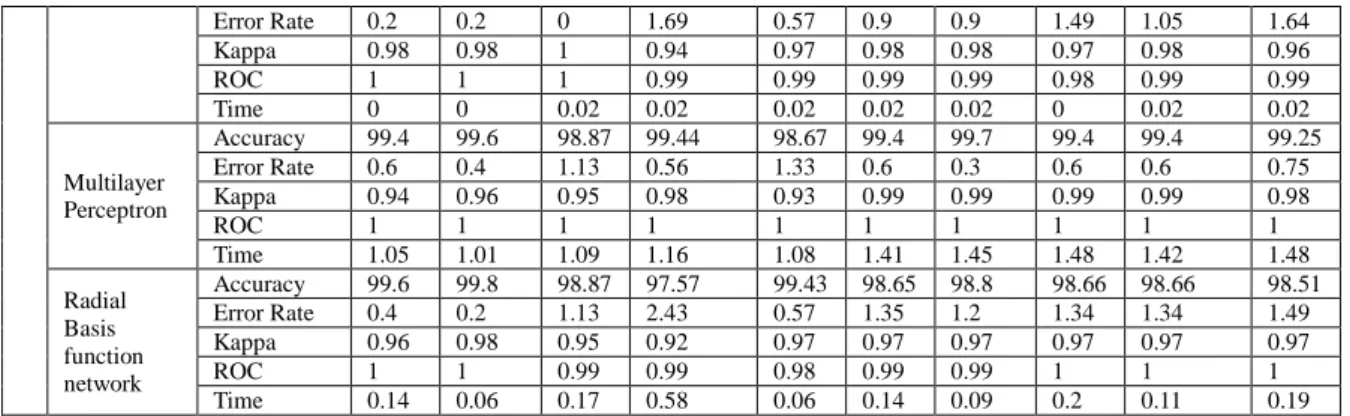
Table 4: Experimental Results of Diabetes and Breast cancer with missing values replaced without applying proposed model

Algorithms Performanc e Estimators

Prediction using K-means with missing values replaced

Diabetes Breast Cancer

Mean Media

n Knn

Weighted

Knn Rpart Mean

Media

n Knn

Weighted

Knn Rpart

S

ta

b

le

Naïve Bayes

Accuracy 98.41 99.2 96.42 95.13 97.53 97.76 97.76 97.91 97.76 97.91

Error Rate 1.59 0.8 3.58 4.87 2.47 2.24 2.24 2.09 2.24 2.09

Kappa 0.87 0.93 0.85 0.85 0.89 0.95 0.95 0.95 0.95 0.95

ROC 1 1 0.99 0.99 1 1 1 1 1 1

Time 0.03 0.02 0.03 0.03 0.03 0.03 0.03 0.03 0.05 0.05

SVM

Accuracy 98.01 99 96.79 97.19 99.05 99.4 99.55 99.4 99.4 99.25

Error Rate 1.99 1 3.21 2.81 0.95 0.6 0.45 0.6 0.6 0.75

Kappa 0.77 0.9 0.84 0.9 0.95 0.99 0.99 0.99 0.99 0.98

ROC 0.82 0.91 0.9 0.94 0.96 0.99 0.99 0.99 0.99 0.99

Time 0.06 0.08 0.25 0.03 0.08 0.06 0.08 0.08 0.08 0.09

K-nn

Accuracy 98.41 98.6 95.85 94.01 96.77 99.7 99.85 99.85 99.85 99.55

Error Rate 1.59 1.4 4.15 5.99 3.23 0.3 0.15 0.15 0.15 0.45

Kappa 0.84 0.87 0.81 0.8 0.83 0.99 1 1 1 0.99

ROC 0.9 0.93 0.91 0.9 0.88 1 1 1 1 1

Time 0 0.02 0 0 0 0 0 0 0 0

U

n

st

ab

le

J48

Accuracy 99.8 99.8 100 98.31 99.43 98.06 98.5 98.36 98.5 99.51

Error Rate 0.2 0.2 0 1.69 0.57 1.94 1.5 1.64 1.5 1.49

Kappa 0.98 0.98 1 0.94 0.97 0.96 0.97 0.96 0.97 0.97

ROC 1 1 1 0.98 0.99 0.98 0.98 0.98 0.98 0.98

Time 0.05 0.02 0.02 0.02 0.03 0.08 0.03 0.02 0.03 0.05

Rep Tree

Accuracy 99.8 99.8 100 98.31 99.81 97.76 97.76 97.62 97.62 97.62

Error Rate 0.2 0.2 0 1.69 0.19 2.24 2.24 2.38 2.38 2.38

Kappa 0.98 0.98 1 0.94 0.99 0.95 0.95 0.95 0.95 0.95

ROC 1 0.98 1 0.98 1 0.98 0.98 0.98 0.98 0.98

Time 0.02 0.02 0 0.03 0.03 0.02 0.03 0.02 0.02 0.02

Ripper

Accuracy 99.6 99.8 99.81 98.88 99.62 98.65 98.66 98.06 98.06 98.21

Error Rate 0.4 0.2 0.19 1.12 0.38 1.35 1.34 1.94 1.94 1.79

Kappa 0.96 0.98 0.99 0.96 0.98 0.97 0.97 0.96 0.96 0.96

ROC 0.98 0.98 0.99 0.99 0.99 0.99 0.99 0.98 0.98 0.98

Time 0.03 0.03 0.06 0.08 0.03 0.08 0.08 0.06 0.06 0.06

(8)

Error Rate 0.2 0.2 0 1.69 0.57 0.9 0.9 1.49 1.05 1.64

Kappa 0.98 0.98 1 0.94 0.97 0.98 0.98 0.97 0.98 0.96

ROC 1 1 1 0.99 0.99 0.99 0.99 0.98 0.99 0.99

Time 0 0 0.02 0.02 0.02 0.02 0.02 0 0.02 0.02

Multilayer Perceptron

Accuracy 99.4 99.6 98.87 99.44 98.67 99.4 99.7 99.4 99.4 99.25

Error Rate 0.6 0.4 1.13 0.56 1.33 0.6 0.3 0.6 0.6 0.75

Kappa 0.94 0.96 0.95 0.98 0.93 0.99 0.99 0.99 0.99 0.98

ROC 1 1 1 1 1 1 1 1 1 1

Time 1.05 1.01 1.09 1.16 1.08 1.41 1.45 1.48 1.42 1.48

Radial Basis function network

Accuracy 99.6 99.8 98.87 97.57 99.43 98.65 98.8 98.66 98.66 98.51

Error Rate 0.4 0.2 1.13 2.43 0.57 1.35 1.2 1.34 1.34 1.49

Kappa 0.96 0.98 0.95 0.92 0.97 0.97 0.97 0.97 0.97 0.97

ROC 1 1 0.99 0.99 0.98 0.99 0.99 1 1 1

Time 0.14 0.06 0.17 0.58 0.06 0.14 0.09 0.2 0.11 0.19

Results after applying Preprocessing:

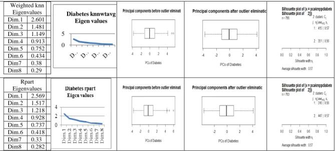
Estimating the Number of PC using Scree Test:

Plotting the eigenvalues against the corresponding PC produces a Scree plot that illustrates the rate of change in the magnitude of the eigenvalues for the PC. The rate of decline tends to be fast first then levels off. The ‘elbow’, or the point at which the curve bends, is considered to indicate the maximum number of PC to extract. One less PC than the number at the elbow will be appropriate for getting an overly defined solution (http://www.ats.ucla.edu/stat/sas/library/factor_ut.htm)

Table 5: Results of Proposed model on diabetes dataset

Diabetes Replacing

method

Scree Plot Before Boxplot

Elimination After Boxplot Elimination

K-means clustering results Mean

Eigenvalues Dim.1 2.3 Dim.2 1.473 Dim.3 1.128 Dim.4 0.928 Dim.5 0.768 Dim.6 0.550 Dim7 0.470 Dim8 0.383

Median Eigenvalues Dim.1 2.283 Dim.2 1.496 Dim.3 1.142 Dim.4 0.917 Dim.5 0.769 Dim.6 0.543 Dim7 0.468 Dim8 0.383

0 2 4

Diabetes median Eigen values

Knn Eigenvalues Dim.1 2.572 Dim.2 1.497 Dim.3 1.146 Dim.4 0.912 Dim.5 0.748 Dim.6 0.432 Dim7 0.403 Dim8 0.290

0 5

D

im

.1

D

im

.2

D

im

.3

D

im

.4

D

im

.5

D

im

.6

D

im

.7

(9)

Weighted knn Eigenvalues Dim.1 2.601 Dim.2 1.481 Dim.3 1.149 Dim.4 0.913 Dim.5 0.752 Dim.6 0.434 Dim7 0.38 Dim8 0.29

0 5

Diabetes knnwtavg Eigen values

Rpart Eigenvalues Dim.1 2.569 Dim.2 1.517 Dim.3 1.218 Dim.4 0.928 Dim.5 0.737 Dim.6 0.418 Dim7 0.33 Dim8 0.282

Experiment using proposed model was conducted on Diabetes and Breast cancer datasets after replacing misssing values using mean,median, Knn,Wt knn and Rpart. In both the cases replacement using Wt knn and Rpart gave same accuracy and improved accuracy when compared with replacing missing values using mean, median and knn therefore results of the proposed model using wtknn is given below.

Table 6: Experimental Results of Diabetes using proposed model

Diabetes Classifiers

Performance Estimators

Prediction of Classifiers without

Preprocessing

Prediction of Classifiers After Preprocessing

(WtKnn replacement + Z-score + PCA + Boxplot outlier elimination + K-means + SVM)

K-means K-means Bagging (No of runs)

Default=10

Adaboost (No of runs) Default=10 Total Instances

Present Absent

534 99 435

510 161 349

S

ta

b

le

C

la

ss

if

ie

rs

Naïve Bayes

Confusion Matrix

present absent present 97 2 absent 24 411

Accuracy 95.13 100 100 100

Error Rate 4.87 0 0 0

Kappa 0.85 1 1 1

NPV 1 1 1 1

Precision 0.8 1 1 1

ROC 0.99 1 1 1

Specificity 0.95 1 1 1

Sensitivity 0.98 1 1 1

FNR(Type II error)

0.02 0 0 0

FPR(Type I error)

0.06 0 0 0

FDR 0.2 0 0 0

FOR 0 0 0 0

Time 0.03 0 0 0

SVM

Confusion Matrix

Accuracy 97.19 100 100 100

Kappa 0.9 1 1 1

NPV 0.98 1 1 1

Precision(PPV) 0.96 1 1 1

ROC 0.94 1 1 1

FNR(Type II error)

0.11 0 0 0

FPR(Type I error)

0.01 0 0 0

(10)

FOR 0.02 0 0 0

Time 1.61 0.05 0.14 0

Knn

Confusion Matrix

Accuracy 94.01 100 100 100

Kappa 0.8 1 1 1

NPV 0.96 1 1 1

ROC 0.9 1 1 1

FNR(Type II error)

0.17 0 0 0

FPR(Type I error)

0.03 0 0 0

FDR 0.15 0 0 0

FOR 0.04 0 0 0

Time 0 0 0.02 0.05

U n st ab le C la ss if ie rs J48 Confusion Matrix present absent present 94 5 absent 4 431

Accuracy 98.31 99.8 99.8 99.8

Error Rate 1.69 0.2 0.2 0.2

Kappa 0.94 1 1 1

NPV 0.99 1 1 1

Precision(PPV) 0.96 0.99 0.99 0.99

ROC 0.98 1 1 1

FNR(Type II error)

0.05 0 0 0

FPR(Type I error)

0.01 0.003 0.003 0.003

FDR 0.04 0.01 0.01 0.01

FOR 0.01 0 0 0

Time 0.03 0.02 0.02 0.02

Rep Tree

Confusion Matrix

Accuracy 98.31 100 100 100

Kappa 0.94 1 1 1

NPV 0.99 1 1 1

ROC 0.98 1 1 1

FNR(Type II error)

0.06 0 0 0

FPR(Type I error)

0.01 0 0 0

FDR 0.03 0 0 0

FOR 0.01 0 0 0

Time 0.03 0.02 0.02 0.02

Ripper

Confusion Matrix

Accuracy 98.88 99.8 99.8 99.8

Error Rate 1.12 0.2 0.2 0.2

Kappa 0.96 1 1 1

NPV 1 1 1 1

ROC 0.99 1 1 1

Sensitivity 0.98 0.99 0.99 0.99

FNR(Type II error)

0.02 0.01 0.01 0.01

FPR(Type I error)

0.01 0 0 0

(11)

FOR 0 0 0 0

Time 0.06 0.03 0.03 0

Part

Confusion Matrix

Accuracy 98.31 99.8 99.8 99.8

Error Rate 1.69 0.2 0.2 0.2

Kappa 0.94 1 1 1

NPV 0.99 1 1 1

Precision(PPV) 0.95 0.99 0.99 0.99

ROC 0.99 1 1 1

FNR(Type II error)

0.04 0 0 0

FPR(Type I error)

0.01 0.003 0.003 0.003

FDR 0.05 0.01 0.01 0.01

FOR 0.01 0 0 0

Time 0.02 0 0.02 0.02

Confusion Matrix

Accuracy 99.44 100 100 100

Kappa 0.98 1 1 1

NPV 0.99 1 1 1

Precision(PPV) 1 1 1 1

ROC 1 1 1 1

Specificity 1 1 1 1

FNR(Type II error)

0.03 0 0 0

FPR(Type I error)

0 0 0 0

FDR 0 0 0 0

FOR 0.01 0 0 0

Time 1.13 0.27 2.02 0.22

Confusion Matrix

Accuracy 97.57 100 100 100

Kappa 0.91 1 1 1

NPV 0.95 1 1 1

ROC 0.99 1 1 1

FNR(Type II error)

0.07 0 0 0

FPR(Type I error)

0.01 0 0 0

FDR 0.06 0 0 0

FOR 0.05 0 0 0

(12)

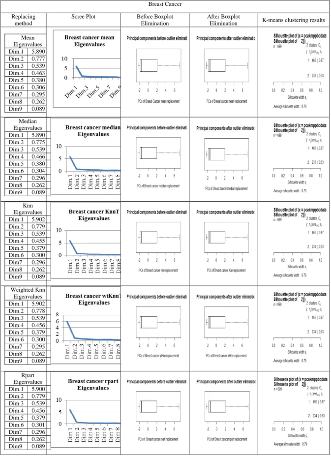
Table 7: Results of Proposed model on Breast Cancer dataset

Breast Cancer Replacing

method

Scree Plot Before Boxplot

Elimination

After Boxplot

Elimination K-means clustering results Mean

Eigenvalues Dim.1 5.890 Dim.2 0.777 Dim.3 0.539 Dim.4 0.463 Dim.5 0.380 Dim.6 0.306 Dim7 0.295 Dim8 0.262 Dim9 0.089

0 5 10

Breast cancer mean Eigenvalues

Median Eigenvalues Dim.1 5.890 Dim.2 0.775 Dim.3 0.539 Dim.4 0.466 Dim.5 0.380 Dim.6 0.304 Dim7 0.296 Dim8 0.262 Dim9 0.089

Knn Eigenvalues Dim.1 5.902 Dim.2 0.779 Dim.3 0.539 Dim.4 0.455 Dim.5 0.379 Dim.6 0.300 Dim7 0.296 Dim8 0.262 Dim9 0.089 Weighted Knn Eigenvalues Dim.1 5.902 Dim.2 0.778 Dim.3 0.539 Dim.4 0.456 Dim.5 0.379 Dim.6 0.300 Dim7 0.295 Dim8 0.262 Dim9 0.089

(13)

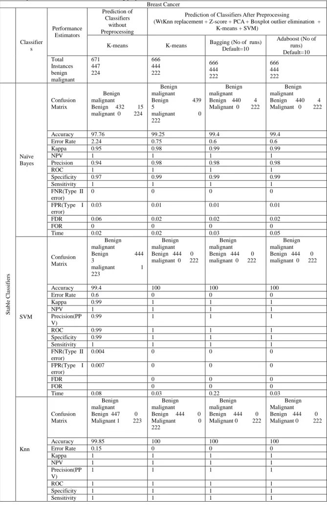
Table 8: Experimental Results of Breast cancer using proposed model Breast Cancer Classifier s Performance Estimators Prediction of Classifiers without Preprocessing

Prediction of Classifiers After Preprocessing

(WtKnn replacement + Z-score + PCA + Boxplot outlier elimination + K-means + SVM)

K-means K-means Bagging (No of runs)

Default=10

Adaboost (No of runs) Default=10 Total Instances benign malignant 671 447 224 666 444 222 666 444 222 666 444 222 S ta b le C la ss if ie rs Naïve Bayes Confusion Matrix Benign malignant

Benign 432 15 malignant 0 224

Benign malignant

Benign 439 5

malignant 0 222

Benign malignant Benign 440 4 Malignant 0 222

Benign malignant

Benign 440 4 Malignant 0 222

Accuracy 97.76 99.25 99.4 99.4

Error Rate 2.24 0.75 0.6 0.6

Kappa 0.95 0.98 0.99 0.99

NPV 1 1 1 1

Precision 0.94 0.98 0.98 0.98

ROC 1 1 1 1

Specificity 0.97 0.99 0.99 0.99

Sensitivity 1 1 1 1

FNR(Type II error)

0 0 0 0

FPR(Type I error)

0.03 0.01 0.01 0.01

FDR 0.06 0.02 0.02 0.02

FOR 0 0 0 0

Time 0.02 0.02 0.03 0.05

SVM

Confusion Matrix

Benign malignant

Benign 444 3

malignant 1 223

Benign malignant Benign 444 0 malignant 0 222

Accuracy 99.4 100 100 100

Kappa 0.99 1 1 1

NPV 1 1 1 1

Precision(PP V)

0.99 1 1 1

ROC 0.99 1 1 1

Sensitivity 1 1 1 1

FNR(Type II error)

0.004 0 0 0

FPR(Type I error)

0.007 0 0 0

FDR 0 0 0

FOR 0 0 0

Time 0.08 0.03 0.22 0.03

Knn

Confusion Matrix

Benign malignant Benign 447 0 Malignant 1 223

Benign malignant

Benign Malignant Benign 444 0 Malignant 0 222

Accuracy 99.85 100 100 100

Kappa 1 1 1 1

NPV 1 1 1 1

Precision(PP V)

1 1 1 1

ROC 1 1 1 1

Specificity 1 1 1 1

(14)

FNR(Type II error)

0.004 0 0 0

FPR(Type I error)

0 0 0 0

FDR 0 0 0 0

FOR 0 0 0 0

Time 0.02 0 0.06 0.06

U n st ab le C la ss if ie rs J48 Confusion Matrix Benign malignant

Benign 440 7

malignant 3 221

Benign malignant

Accuracy 98.5 99.85 99.85 99.85

Error Rate 1.5 0.15 0.15 0.15

Kappa 0.97 1 1 1

NPV 0.99 1 1 1

Precision(PP V)

0.97 1 1 1

ROC 0.98 1 1 1

FNR(Type II error)

0.013 0 0 0

FPR(Type I error)

0.016 0.002 0.002 0.002

FDR 0.03 0 0 0

FOR 0.01 0 0 0

Time 0.05 0 0.02 0.02

Rep Tree Confusion Matrix Benign malignant Benign 438 9 malignant 7 217

Benign malignant

Benign 444 0

malignant 0 222

Benign malignant

Accuracy 97.62 100 100 100

Kappa 0.95 1 1 1

NPV 0.98 1 1 1

Precision(PP V)

0.96 1 1 1

ROC 0.98 1 1 1

FNR(Type II error)

0.03 0 0 0

FPR(Type I error)

0.02 0 0 0

FDR 0 0 0

FOR 0 0 0

Time 0.03 0 0 0.02

Ripper

Confusion Matrix

Benign malignant

Accuracy 98.06 99.85 99.85 99.85

Error Rate 1.94 0.15 0.15 0.15

Kappa 0.96 1 1 1

NPV 0.98 1 1 1

Precision(PP V)

0.98 1 1 1

ROC 0.98 1 1 1

FNR(Type II error)

0.04 0.01 0.01 0.01

FPR(Type I error)

0.01 0 0 0

FDR 0.02 0 0 0

(15)

Time 0.08 0.02 0.02 0.02

Part

Confusion Matrix

Benign malignant

Accuracy 98.96 99.85 99.85 99.85

Error Rate 1.04 0.15 0.15 0.15

Kappa 0.98 1 1 1

NPV 0.99 1 1 1

Precision(PP V)

0.98 1 1 1

ROC 0.99 1 1 1

FNR(Type II error)

0.01 0 0 0

FPR(Type I error)

0.01 0.002 0.002 0.002

FDR 0.02 0 0 0

FOR 0.01 0 0 0

Time 0.02 0 0.02 0

Multilaye r Perceptro n

Confusion Matrix

Benign malignant

Accuracy 99.4 100 100 100

Kappa 0.99 1 1 1

NPV 1 1 1 1

Precision(PP V)

0.99 1 1 1

ROC 1 1 1 1

Sensitivity 1 1 1 1

FNR(Type II error)

0.004 0 0 0

FPR(Type I error)

0.007 0 0 0

FDR 0.01 0 0 0

FOR 0 0 0 0

Time 1.42 0.3 2,64 0.28

Confusion Matrix

Benign malignant

Benign 438 9

malignant 0 224

Accuracy 98.66 99.85 99.85 99.7

Error Rate 1.34 0.15 0.15 0.3

Kappa 0.97 1 1 0.99

NPV 1 1 1 1

Precision(PP V)

0.96 1 1 0.99

ROC 1 1 1 1

Sensitivity 1 1 1 1

FNR(Type II error)

0 0 0 0

FPR(Type I error)

0.02 0.002 0.002 0.01

FDR 0.04 0 0 0.01

FOR 0 0 0 0

Time 0.09 0.09 0.41 0.39

(16)

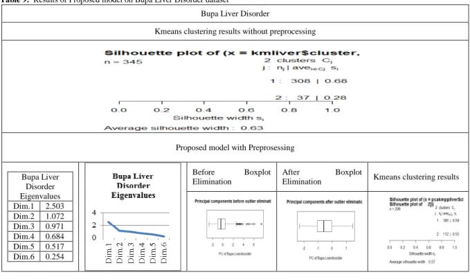
Table 9: Results of Proposed model on Bupa Liver Disorder dataset

Bupa Liver Disorder

Kmeans clustering results without preprocessing

Proposed model with Preprosessing

Bupa Liver Disorder Eigenvalues Dim.1 2.503 Dim.2 1.072 Dim.3 0.971 Dim.4 0.684 Dim.5 0.517 Dim.6 0.254

Before Boxplot Elimination

After Boxplot

Elimination Kmeans clustering results

Table 10: Experimental Results of Bupa Liver Disorder using proposed model Bupa Liver Disorder

Classifiers

Performance Estimators

Prediction of Classifiers

without Preprocessing

Prediction of Classifiers After proposed Preprocessing (Z-score + PCA + Boxplot outlier elimination + K-means + SVM) Total Instances

absent present

191 177 14

153 67 86

K-means K-means Bagging (No of

runs)

Adaboost (No of runs)

S

ta

b

le

C

la

ss

if

ie

rs

Naïve Bayes

Confusion Matrix

absent present absent 169 8 present 1 13

Accuracy 95.29 100 100 100

Kappa 0.72 1 1 1

NPV 0.99 1 1 1

ROC 0.99 1 1 1

FNR(Type II error)

0.07 0 0 0

FPR(Type I error)

0.05 0 0 0

FDR 0.38 0 0 0

FOR 0.01 0 0 0

Time 0.02 0 0.02 0

SVM

Confusion Matrix

Accuracy 95.29 98.69 100(50) 98.69

Error Rate 4.71 1.31 0 1.31

Kappa 0.51 0.97 1 0.97

NPV 0.95 1 1 1

Precision(PPV) 1 0.98 1 0.98

ROC 0.68 0.99 1 1

Specificity 1 0.97 1 0.97

(17)

error) FPR(Type I error)

0 0.03 0 0.03

FDR 0 0.02 0 0.02

FOR 0.05 0 0 0

Time 0.02 0.02 0.48 0.05

Knn

Confusion Matrix

Accuracy 97.91 100 100 100

Kappa 0.82 1 1 1

NPV 0.98 1 1 1

Precision(PPV) 1 1 1 1

ROC 0.88 1 1 1

Specificity 1 1 1 1

FNR(Type II error)

0.286 0 0 0

FPR(Type I error)

0 0 0 0

FDR 0 0 0 0

FOR 0.02 0 0 0

Time 0 0 0 0

U n st a b le C la ss if ie rs J48 Confusion Matrix

Accuracy 97.38 99.35 99.35 99.35

Error Rate 2.62 0.65 0.65 0.65

Kappa 0.8 0.99 0.99 0.99

NPV 0.98 0.99 0.99 0.99

ROC 0.92 0.99 0.99 0.99

Sensitivity 0.79 0.99 0.99 0.99

FNR(Type II error)

0.21 0.01 0.01 0.01

FPR(Type I error)

0.01 0 0 0

FDR 0.15 0 0 0

FOR 0.02 0.01 0.01 0.01

Time 0.02 0.02 0 0.02

Rep Tree

Confusion Matrix

Accuracy 97.38 100 100 100

Kappa 0.8 1 1 1

NPV 0.98 1 1 1

ROC 0.88 1 1 1

FNR(Type II error)

0.21 0 0 0

FPR(Type I error)

0.01 0 0 0

FDR 0.15 0 0 0

FOR 0.02 0 0 0

Time 0.03 0 0.03 0

Ripper

Confusion Matrix

Accuracy 96.34 99.35 99.35 99.35

Error Rate 3.66 0.65 0.65 0.65

Kappa 0.72 0.99 0.99 0.99

NPV 0.98 1 1 1

(18)

ROC 0.85 0.99 1 0.99

Specificity 0.98 0.99 0.99 0.99

FNR(Type II error)

0.29 0 0 0

FPR(Type I error)

0.02 0.02 0.02 0.02

FDR 0.23 0.01 0.01 0.01

FOR 0.02 0 0 0

Time 0.02 0 0.03 0

Part

Confusion Matrix

Accuracy 97.38 99.35 99.35 99.35

Error Rate 2.62 0.65 0.65 0.65

Kappa 0.8 0.99 0.99 0.99

NPV 0.98 0.99 0.99 0.99

ROC 0.92 0.99 0.99 0.99

Sensitivity 0.79 0.99 0.99 0.99

FNR(Type II error)

0.21 0.01 0.01 0.01

FPR(Type I error)

0.01 0 0 0

FDR 0.15 0 0 0

FOR 0.02 0.01 0.01 0.01

Time 0 0 0 0.02

Confusion Matrix

Accuracy 98.95 100 100 100

Kappa 0.92 1 1 1

NPV 0.99 1 1 1

ROC 1 1 1 1

FNR(Type II error)

0.07 0 0 0

FPR(Type I error)

0.01 0 0 0

FDR 0.07 0 0 0

FOR 0.01 0 0 0

Time 0.31 0.11 0.65 0.08

Confusion Matrix

Accuracy 98.43 100 100 100

Kappa 0.88 1 1 1

NPV 0.99 1 1 1

ROC 0.99 1 1 1

FNR(Type II error)

0.14 0 0 0

FPR(Type I error)

0.01 0 0 0

FDR 0.08 0 0 0

FOR 0.01 0 0 0

(19)

Table 11: Summary of clustering validations

Dataset Replace

method

Before preprocessing After Preprocessing (Scaling+ PCA+ Boxplot

Elimination) Total No of Instance s Cluste r No No of Instances Silhouett e coefficie nt Rand Inde x No of Instance s Cluste r No No of Instance s Silhouett e coefficie nt Rand Index Diabete

s Mean

768 1 715 0.73 0.65

5

766 1 360 0.55 0.711

2 53 0.37 2 406 0.56

Median 768 1 712 0.75 0.65

4

766 1 343 0.55 0.718

2 56 0.4 2 423 0.56

Knn 768 1 98 0.31 0.69 766 1 418 0.57 0.719

2 670 0.64 2 348 0.55

Weighte d Knn

768 1 164 0.33 0.7 766 1 415 0.57 0.718

2 604 0.6 2 351 0.56

Rpart 768 1 93 0.45 0.68₆ 766 1 316 0.56 0.721

2 675 0.67 2 447 0.57

Wiscos in Breast cancer

Mean 699 1 466 0.75 0.95₇ 699 1 466 0.87 0.954

2 233 0.28 2 233 0.63

Median 699 1 465 0.76 0.95₉ 699 1 466 0.87 0.954

2 234 0.28 2 233 0.63

Knn 699 1 464 0.76 0.95

9

699 1 465 0.87 0.956

2 235 0.28 2 234 0.63

Weighte dKnn

699 1 464 0.76 0.95

9

699 1 465 0.87 0.956

2 235 0.28 2 234 0.63

Rpart 699 1 464 0.76 0.95

9

699 1 465 0.87 0.956

2 235 0.28 2 234 0.63

Bupa Liver disorde r No missing values

345 1 37 0.28 0.55

4

298 1 186 0.59 0.523

2 308 0.68 2 112 0.55

Table 12: Summary of Preprocessing

Data sets No of

instances

Method selected

for replacing

missing values

No of Principal Components Selected According To Scree plot

No of instances after Boxplot Elimination

No of

correctly clustered instances using K-means

% of Error

No of

instances after Svm Optimization

Diabetes 768 Weighted

Knn 1 766 550 28.2 510

Wiscosin

Breast cancer 699

Weighted

Knn 1 699 668 4.43 666

Bupa Liver

disorder 345

Weighted

Knn 1 298 156 47.65 153

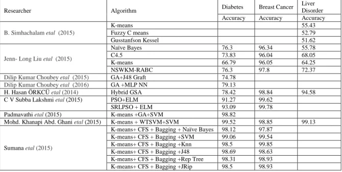
Table 13: Comparison of Results with other methods and Proposed Model for Diabetes, Breast Cancer and Bupa Liver disorder

Researcher Algorithm Diabetes Breast Cancer

Liver Disorder Accuracy Accuracy Accuracy B. Simhachalam etal (2015)

K-means 55.43

Fuzzy C means 52.79

Gusstanfson Kessel 51.62

Jenn- Long Liu etal (2015)

Naïve Bayes 76.3 96.34 55.78

C4.5 73.83 96.04 68.05

K-means 66.79 96.05 64.25

NSWKM-RABC 76.3 97.8 72.37

Dilip Kumar Choubey etal (2015) GA+J48 Graft 74.78 Dilip Kumar Choubey etal (2016) GA +MLP NN 79.13

H. Hasan ÖRKCÜ etal (2014) Hybrid GSA 78.42 98.84 94.58

C V Subba Lakshmi etal (2015) PSO+ELM 91.27 99.62

SRLPSO + ELM 93.09 99.78

Padmavathi etal (2015) K-means +GA+SVM 98.82

Mohd. Khanapi Abd. Ghani etal (2015) K-means + WTSVM+SVM 99.52 98.85 99.13

Sumana etal (2015)

K-means+ CFS + Bagging + Naïve Bayes 98.12 97.87

K-means+ CFS + Bagging +SVM 99.06 99.54

K-means+ CFS + Bagging +Knn 98.5 99.85

K-means+ CFS + Bagging +J48 98.69 98.63

K-means+ CFS + Bagging +Rep Tree 98.31 98.93

(20)

K-means+ CFS + Bagging +Part 98.5 98.93

K-means+ CFS + Bagging +MLP 99.81 99.54

K-means+ CFS + Bagging +RBF 99.44 98.63

Sumana etal (2015)

K-means+ CFS + Adaboost + Naïve Bayes

99.44 99.54

K-means+ CFS + Adaboost +SVM 99.25 99.24

K-means+ CFS + Adaboost +Knn 98.5 99.85

K-means+ CFS + Adaboost +J48 99.25 99.09

K-means+ CFS + Adaboost +Rep Tree 98.12 99.09

K-means+ CFS + Adaboost +JRip 98.5 99.39

K-means+ CFS + Adaboost +Part 98.87 99.23

K-means+ CFS + Adaboost +MLP 99.44 99.54

K-means+ CFS + Adaboost +RBF 99.62 99.54

Sambasiva Rao Voleti etal ( 2015)

Kmeans + Naïve Bayes 99.3 97.6

Kmeans + Back Propagation. 100 100

Kmeans + SVM 100 99.1

Sumana etal (2015)

Proposed model with Naïve Bayes Proposed model with Bagging/Adaboost + Naïve Bayes

100 99.25

99.4

100

Proposed model with SVM 100 100 98.69

Proposed model with Knn 100 100 100

Proposed model with J48 99.8 99.85 99.35

Proposed model with Rep Tree 100 100 100

Proposed model with JRip 99.8 99.85 99.35

Proposed model with Part 99.8 99.85 99.35

Proposed model with MLP 100 100 100

Proposed model with RBF 100 99.85 100

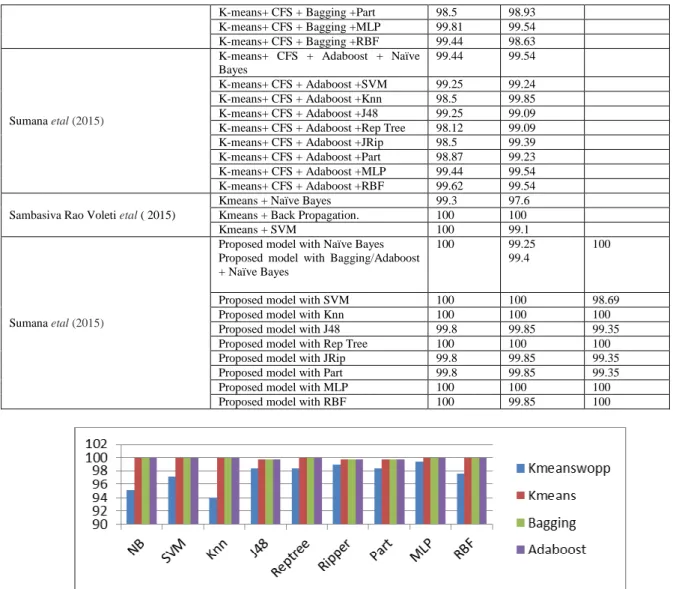
Fig. 2: Comparison of proposed model and without proposed model for Pima Indian Diabetes dataset

Fig. 3: Comparison of proposed model and without proposed model for Breast cancer dataset

(21)

Research Findings:

1. Though previous researches proved that hybrid clustering and classification gives good accuracy over individual classification and clustering, researchers are confused to select a clustering algorithm for a particular dataset. The proposed model has removed that confusion and clearly gives a suggestion that K-means with few preprocessing steps like scaling, finding Principal components using PCA and outlier elimination before K-means followed by SVM optimization is a good one.

2. The objective of the work was to reduce the Type II error is achieved

3. Preprocessing is so effective that there is no scope for ensemble to improve the classifier accuracy as all algorithms behaves to be stable i.e., ensemble Bagging and Boosting using the proposed model did not improve the accuracy of any classifier.

4. Ensemble models are too complex (Sumana et al., 2014) therefore can be avoided using the proposed model with few preprocessing steps before clustering.

5. The preprocessing steps in the proposed model is so effective that there is no scope for the ensemble model

6. In the proposed hybrid clustering and classification preprocessing and outlier elimination followed by SVM optimization before clustering improves the efficiency of clustering algorithm which finally improves the accuracy of the classifier.

7. The proposed model is the ideal model for Knn, MLP and RepTree as its accuracy was 100% on all data sets.

8. The time taken by MLP using the proposed model is very less

Conclusion:

The time taken for this hybrid model is very less compared to the individual clustering and classification. In the literature there are many papers discussing about different clustering algorithm for different datasets and previous researches (Sumana et al., 2014, Karegowda et al., 2012, Sumana et al., 2015) proved that hybrid clustering and classification has an improvement over the traditional classification and clustering. Though K-means is the best proven algorithm by most of the researchers, there is no single paper suggesting the best clustering algorithm for all the data sets. The proposed model was successful in providing a suggestion for the researchers getting confused in the selection of the clustering algorithm. This proposed model was successful in proving that K-means with proper preprocessing enhances the classifiers and there is no need for ensemble model.

This paper, empirically studies the impact of preprocessing before clustering enhancing the classifier accuracy by overcoming the issues discussed in the background problem. The proposed model was tested on 3 different datasets and was not only able to prove that proper preprocessing before clustering enhances the classifier accuracy it also provided few guidelines for each issue discussed in the background problem. 1) PCA was adapted in this proposed model to overcome the issue that K-means is not suitable for high dimensional data therefore PCA was used to reduce to a lower dimension. 2) Presence of outliers deviate the cluster centroids thus degrades the performance of K-means hence Boxplot was adapted in this proposed model to overcome this issue. As both PCA and K-means efficiency depends on numeric values the data was normalized before performing PCA and K-means so that higher attribute values should not dominate the lower attribute values. Since the efficiency of K-means is sensitive to the initialization of the cluster centroid experiment was tried using K-means++ and Hybrid Hierarchical and K-means clustering where the centroid for K-means was initialized using the Hierarchical algorithm but it did not improve the performance of clustering algorithm. The performance of K-means using Lloyd, K-means++ and Hierarchical K-means resulted in same performance. Finally to optimize the efficiency of means, SVM was used to remove the misclassified instances of K-means. SVM was adapted as an optimizing algorithm because the data sets used are binary classification problem.

Accuracy of the classifier in the proposed model depends on the efficiency of the clustering algorithm therefore the future work will make an attempt to enhance the accuracy of the clustering algorithm and also will explore to test the proposed model on data sets in other domains as well as with categorical attributes and non-linear data sets to judge the performance of the proposed model. Further the future work will experiment the use of feature selection algorithms to select significant attributes, process to eliminate balancing and try to use regression models for prediction.

Contributions:

(22)

REFERENCES

Angel Latha Mary, S., A.N. Sivagami and M. Usha Rani, 2015. Cluster Validity Measures Dynamic Clustering Algorithms. ARPN Journal of Engineering and Applied Sciences, 10(9): 4009-4012.

Choubey, Dilip Kumar and Sanchita Paul, 2015. GA_J48graft DT: A Hybrid Intelligent System for Diabetes Disease Diagnosis. SERSC: International Journal of Bio-Science and Bio-Technology, pp: 2233-7849.

Choubey, Dilip Kumar, and Sanchita Paul, 2016. GA_MLP NN: A Hybrid Intelligent System for Diabetes Disease Diagnosis, I.J. Intelligent Systems and Applications, 1: 49-59.

Hasan ÖRKCÜ1, H., Mustafa Đ_{sa DO}Ğ_{AN and Mediha ÖRKCÜ Gazi, 2015. A Hybrid Applied}

Optimization Algorithm for Training Multi-Layer Neural Networks in Data Classification, Gazi University Journal of Science, 28(1): 115-132.

Howley, Tom, Michael, G. Madden, Marie-Louise O’Connell and Allan G. Ryder, 2006. The effect of principal component analysis on machine learning accuracy with high-dimensional spectral data. Knowledge-Based Systems, 19(5): 363-370.

http://www.ats.ucla.edu/stat/sas/library/factor_ut.htm

Janecek, Andreas, G.K. and Wilfried N. Gansterer, 2008. A Comparison of Classiffication Accuracy Achieved with Wrappers, Filters and PCA. Workshop on New Challenges for Feature Selection in Data Mining and Knowledge Discovery, pp: 1-12.

Jenn-Long Liu and Chung-Chih Li., 2015. A Non-symmetrical Weighted K-means with Rank-Based Artificial Bee Colony Algorithm for Medical Diagnosis, International Journal of Machine Learning and Computing, 5(4): 264-270.

Karegowda, Asha Gowda., M.A. Jayaram and A.S. Manjunath, 2012. Cascading means clustering and k-nearest neighbor classifier for categorization of diabetic patients. International Journal of Engineering and Advanced Technology, 1(3): 147-151.

Minakshi, Dr. Rajan Vohra, Gimpy, 2014. Missing Value Imputation in Multi Attribute Data Set (IJCSIT) International Journal of Computer Science and Information Technologies, 5(4): 5315-5321

Mohd. Khanapi Abd. Ghani and Daniel Hartono Sutanto, 2015. Improving classification accuracy for Non-Communicable disease prediction Model Based on support Vector Machine, Jurnal Teknologi (Sciences & Engineering) 77(18): 29-36.

Pavel., Mircea-SerbanSattaro, Timur, 2015. On the importance of preprocessing and initialization in k-means ResearchGate

Prabha. K and K. Rajeswari, 2014. A Hybrid approach for Data Clustering using Data mining techniques. International Journal of Computer Science and Mobile Computing, 3(11): 81-88.

Sambasiva Rao Voleti and Kiran Kumar Reddi, 2015. Classifiers Performance Improvement through Integration of Clustering Technique, International Journal of Advanced Research in Computer Science and Software Engineering, 5(5): 808-813.

Santhanam, T and Padmavathi, M.S., 2015. Application of K-Means and Genetic Algorithms for Dimension Reduction by Integrating SVM for Diabetes Diagnosis, Procedia Computer Science, 47: 76-83.

Saranya, C. and G. Manikandan, 2013. A study on normalization techniques for privacy preserving data mining. International Journal of Engineering and Technology (IJET) 5(3): 2701-2704.

Simhachalam, B and G. Ganesan, 2015. Performance comparison of fuzzy and non-fuzzy classification methods. Egyptian Informatics Journal., pp: 1-6.

Sindhupriya, R amd X. Ignatius Selvarani, 2014. K-means based Clustering in Higher Dimensional Data. .International Journal of Advanced Research in Computer Engineering and Technology, 3(2): 432-436.

Somasundaram, R.S. and R. Nedunchezhian, 2011. Evaluation of three simple imputation methods for enhancing preprocessing of data with missing values. International Journal of Computer Applications, 21(10): 14-19.

Subbulakshmi and S.N. Deepa, 2015. Medical Dataset Classification: A Machine Learning Paradigm Integrating Particle Swarm Optimization with Extreme Learning Machine Classifier, The Scientific World Journal, pp: 1-12.

Sumana, B.V and T. Santhanam, 2014. An Empirical Comparison of Ensemble and Hybrid Classification Proc. Processing and VLSI. pp: 463-470.

Sumana, B.V and T. Santhanam, 2014. Prediction of diseases by cascading clustering and classification. Advances in Electronics, Computers and Communications (ICAECC), International Conference on. IEEE.

Sumana, B.V and T. Santhanam, 2015. Optimizing the Prediction of Bagging and Boosting. Indian Journal of Science and Technology, 8(35): 1-13.

UCI repository of machine learning databases. Irvine, CA: University of California, Department of Information science and ComputerScience.{http://www.ics.uci.edu/~mlearnMLRepository.html}1998.

(23)

Venkatesan, Anusuya and Latha Parthiban, 2011. Clustering of datasets using PSO-K-Means and PCA-K-means. International Journal of Computational Intelligence and Informatics., 1: 180-184.

Ville Hautamäki, Svetlana Cherednichenko, Ismo Kärkkäinen, Tomi Kinnunen and Pasi Fränti, 2005. Improving k-means by outlier removal. Image Analysis. Springer Berlin Heidelberg, pp: 978-987.

wikipedia.org/wiki/Matthews_correlation_coefficient