Sharif University of Technology
Scientia IranicaTransactions E: Industrial Engineering http://scientiairanica.sharif.edu
Cost function and optimal boundaries for a two-level
inventory system with information sharing and two
identical retailers
A.H. Afshar Sedigh
a, R. Haji
b, and S.M. Sajadifar
c;a. Department of Information Science, University of Otago, Dunedin 9054, P.O. Box 56, New Zealand. b. Department of Industrial Engineering, Sharif University of Technology, Tehran, P.O. Box 11365, Iran. c. Department of Industrial Engineering, University of Science and Culture, Tehran, P.O. Box 13145/871, Iran. Received 21 September 2016; received in revised form 22 May 2017; accepted 20 June 2018
KEYWORDS Two-echelon inventory system;
Supply chain management; Information sharing; Poisson demand; Continues review.
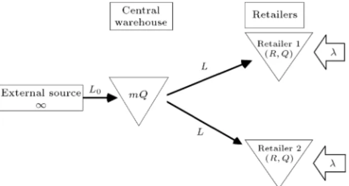
Abstract. In this paper, we consider a two-echelon inventory system with a central warehouse and two identical retailers employing information sharing. Transportation times to each retailer and the warehouse are constant. Retailers face independent Poisson demand and apply continuous review policy, i.e., (R; Q)-policy. The warehouse initiates with m batches (of given size Q) and places an order with an outside supplier when a retailer's inventory position reaches R + s; R + s is the inventory position considered by the central warehouse and s is a non-negative constant. So far, an approximate cost function as well as exact analysis of system for only one retailer has been proposed. However, the derivation of the exact value of the expected total cost of the system for more than one retailer is still an open question. This paper attempts to meet this challenge and derive the exact cost function for two retailers. To achieve this purpose, we resort to conditional probability to split the problem into two simpler problems; then, we obtain the exact expected total cost of the system.
© 2019 Sharif University of Technology. All rights reserved.
1. Introduction
In an uncertain, complicated, and competitive market, it is vital for a business to improve its exibility and approachability. To satisfy these needs, companies have concentrated on information technology at an increasingly fast pace. On the other hand, distribution of benets among members creates a tendency to share their information. If there is a fair distribution of benets among all members, or all decisions are made
*. Corresponding author.
E-mail addresses: [email protected] (A.H. Afshar Sedigh); [email protected] (R. Haji);
[email protected] (S.M. Sajadifar) doi: 10.24200/sci.2018.20144
by one party, they will use a centralised decision-making system. When members are independent and operate as separate parties, these systems are regarded as decentralised supply chain systems.
When there is no information sharing throughout the supply chain, each level aims to optimise its costs. As a result, customer demand variability tends to increase for upstream level parties (vendors, manu-facturers, etc.) In the literature, this phenomenon is known as bullwhip eect. Forrester [1] reported this situation for the rst time and referred to it as \Demand Amplication." Afterwards, bullwhip eect was shown in games; the most recognised of such games was \Beer Distribution Game," also known as \Beer Game," created by Forrester and others at MIT. Thereafter, electronic versions and web-based versions were proposed by Simchi-Levi et al. [2].
Nowadays, we have at our disposal the results of extensive empirical and theoretical studies about the values of information sharing. Lee et al. [3] considered a two-echelon supply chain including one manufacturer and one retailer for periodic review in-ventory system. Their analysis showed the impact of information sharing on reducing the inventory and cost levels. They also found out that demand process and transportation time had an extensive inuence on the advantages of information sharing. Raghu-nathan and Yeh [4] studied the eect of Continuous Replenishment Program (CRP) on the system pro-posed by Lee et al.; the presented results showed that for demands with wide variation and small mean, information sharing was more valuable than CRP. Yao and Dresner [5] developed the models proposed by Lee et al. and Raghunathan and Yeh to examine the value of information sharing under CRP and Vendor Managed Inventory (VMI). They concluded that CRP and VMI were more benecial to the retailer and the manufacturer, respectively. Recently, Dong et al. [6] studied collaborative supply chain management employing an item-level dataset and indicated that the downstream rm gained signicant benets as a result of the decision-transfer inherited from VMI. Cui et al. [7] investigated value of information in a two-echelon supply chain where the decision maker had the permission to change the policy dynamically. Using this approach depicted the eciency of information sharing as well as reconciliation of theoretical and empirical ndings.
In a study, Chen et al. [8] considered eight scenarios with respect to three dierent types of formation, i.e. demand, inventory, and capacity in-formation. These scenarios were designed based on the used information. Their analysis showed that full information sharing had the best performance among other scenarios. Razmi et al. [9] compared traditional information sharing and VMI information sharing sys-tems. They proved that VMI was more advantageous than the traditional approach. Li [10] proposed a exible method of information sharing in a supply chain where parties could share limited information to other members of supply chain. They performed simulation and quantitative analysis and it was concluded that even limited information sharing would enhance supply chain performance.
Moreover, in [11], a four-echelon supply chain with partial information sharing was simulated. The authors concluded that more information sharing en-hanced the system performance; also, increase in col-laborating members was an eective factor regardless of their roles. Canella et al. [12] studied the variety of information that could be shared by supply chain parties, i.e. real-time point-of-sale, sales forecasts, and inventory order policies and reports, to improve
their performance using a continuous time domain simulation. In [13], Canella and Ciancimino addressed make-to-stock supply chain managing by (S; R) and proposed a novel order-up-to policy for the afore-mentioned system when parties were coordinated by sharing information. Cannella [14] investigated the enhancement introduced into the supply chain by re-placing conventional myopic periodic inventory review with Automatic Pipeline Variable Inventory and Or-der Based Production Control System (APVIOBPCS) policy when demand was normal.
In more recent studies, Prajogo and Olhager [15] investigated the inuence of information sharing in a three-echelon supply chain. Extra demand was backlogged and three levels of information sharing were considered. They concluded that increase in information sharing level resulted in expected cost reduction. Ganesh et al. [16] analysed the value of information sharing in a multi-level supply chain con-sidering various products with multiple levels of sub-stitutability. Their results indicated that if upstream members ignored substitution or demand correlation, they might overestimate the information sharing value. Sabitha et al. [17] studied the value of information sharing in a multi-stage supply chain with one item and non-zero lead time. They found out that the vendor managed inventory and supply-chain-wide information sharing were the same and upstream companies ben-eted more from this policy. Ali et al. [18] and Babai et al. [19] addressed the value of information sharing in forecasted demand. These two studies indicated that demand process aected the value of information sharing and this value highly diminished in auto-correlated demand. Trapero et al. [20] studied information sharing benet to forecast improvement. They analysed weekly data of a manufacturer and a major retailer in UK. This study emphasised that information sharing enhanced forecasting accuracy. In a more recent attempt, Cannella et al. [21] simulated a serially linked supply chain consisting of k echelons with decentralised coordination and showed that the collaboration improved service levels of both customers and upstream members of supply chain as well as process eciency of members.
In the rest of the paper, we concentrate on two-level inventory systems with stochastic demand and centralised decision-making system. We also narrow down literature review to systems which use continuous review. Li and Wang [22] categorised the proposed methods to handle these systems as follows:
I. Installation stock policies: In these policies, no information about buyers is utilised by the sup-plier. This property makes them easy to operate, but excludes system performance optimisation. Axsater [23] proposed a basic model and its
optimisation for a two-echelon system controlled by a base stock policy using inventory position. Furthermore, Axsater [24] extended the former model to a batch ordering system for two retailers and suggested an approximation for more than two retailers. Afterwards, Forsberg [25] presented a model and its optimisation for systems which used order up to-S policy with a compound Poisson demand. He showed that demands could be used instead of inventory positions in the basic model proposed by Axsater. Forsberg [26] also evaluated the exact cost function for a two-echelon system with continuous review policy, Poisson demand, and non-identical batch sizes. Axsater [27] presented a more generalised model for ordering up to-S policy when demand process was compound Poisson with various ordering size. Further review of stochastic multiproduct systems and evaluating cost using queuing systems were performed by Simchi-Levi and Zhao [28,29].
II. Echelon stock policies: In these systems, a party has information about cumulative inventory po-sition of all related downstream parties. Chen and Zheng [30] evaluated (R; nQ) echelon stock policies in serial inventory systems; they modied an approximation for these systems as well. Chen and Zheng [31] extended this problem to a mul-tistage inventory system with compound Poisson demand and evaluated optimum boundaries, and proposed an algorithm for a near optimal solution. Axsater and Rosling [32] compared echelon stock and installation stock policies in multi-echelon inventory systems. They concluded that even for the worst scenarios, echelon stock policy was as eective as installation stock policy.
III. Information sharing: In these systems, based on managers' policy, all or part of the informa-tion about inventory posiinforma-tion, Bill Of Materials (BOM), etc. is shared among members. As it is discussed by Simchi-Levi et al. [2], information sharing can enhance cost savings due to a reduc-tion in the forecast errors which the retailers deal with. The objective of information sharing as a part of information technology is to help supply managers not only to secure transparency and accessibility of information but also to make deci-sions based on the total supply chain information. Moinazadeh [33] studied a supply chain including a product, a central warehouse, and some identical retailers under a stationary random demand. In this model, retailers used (R; Q) ordering policy. He recom-mended an ordering policy for the central warehouse using the real-time information about each retailer's inventory position with the central warehouse placing an order with an external supplier when a retailer's
inventory position reached R + s(0 s Q 1). To evaluate the system costs and derive the optimal policy, an approximate model and a heuristic optimization were proposed for this policy.
Haji and Sajadifar [34] derived the exact cost function for the policy proposed by Moinzadeh (2002) considering one retailer. They used Axsater (1990) installation stock model for one-for-one policy, to evaluate the cost function. Following this study, Sajadifar and Haji [35] derived the optimal boundaries for their proposed model such that their optimisation procedure required less computational eort and was directed towards the optimal solution. In a more recent study, Axsater and Marklund [36] proposed an information sharing policy for non-identical retailers in which demand was a coecient of a standard batch size and, as previously established, concluded that information sharing lowered the system costs.
In this paper, we evaluate system costs for the policy presented by Moinzadeh (2002) when there are two identical retailers, which has been an open question ever since. A brief schema of the problem is illustrated in Figure 1. The proposed method by Moinzadeh (2002) obtained neither the exact model nor the optimal boundaries of the policy. Moreover, he used a heuristic algorithm that could not guarantee obtaining the optimal solution. To overcome the aforementioned issues, we propose the exact model and optimal boundaries. Therefore, we rst propose an illustrative example for this problem to attain better understanding of system complexities, special cases, and dierent system states. Afterwards, we consider an arbitrary batch (Q0) and divide the problem into some
easier sub-problems to derive the probability function for demands needed to order this batch. Subsequently, we propose upper bound and lower bound of optimum solution and the cost function of the system under study.
The rest of this paper is organised as follows. The problem is dened in Section 2 by proposing its assumptions and notations. In Section 3, an illustrative example is presented for more clarication of
complex-Figure 1. A schema of a two-echelon system with two retailers and a central warehouse.
ities and diculties of modelling. Section 4 derives the probability distribution required for cost function calculation. The boundaries of optimal solution are proposed in Section 5. Section 6 represents the nal model and its optimisation method. Finally, Section 7 represents the conclusion and some future directions for research.
2. Problem denition
In this section, employed notations and assumptions of this paper are represented. We utilise similar notations to those of Axsater (1990) and Moinzadeh (2002) for ease of researchers familiar with these papers.
2.1. Notations
The adopted notations are as follows (similar to [33]): L Carrying time from the central
warehouse to each retailer; L0 Carrying time from the external
supplier to the central warehouse; Demand intensity at each retailer; h Holding cost per unit per unit time at
each retailer;
h0 Holding cost per unit per unit time at
the central warehouse;
Shortage cost per unit per unit time at each retailer;
Q Given system's order quantity; R Reorder point for each one of the
retailers;
m Number of initial batches allocated to the central warehouse.
Also, we use the following notations based on [23]: (S0) Average holding cost in the central
warehouse per unit when the inventory position at warehouse is S0;
S(S
0) Average holding and shortage cost in
a retailer when inventory positions of the central warehouse and retailer are S0 and S, respectively.
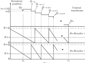
The rest of the notations are as follows (for an example, see Figure 2):
Q0 The arbitrary batch chosen for
investigation;
t0 Ordering time of Q0 by the central
warehouse;
t1 Ordering time of Q0 by one of the
retailers;
B The retailer which orders Q0;
t+ A moment after t;
Figure 2. An example of the system.
t A moment before t;
k Customer demand from t0 until t+1;
j Arbitrary unit of Q0;
T C(m; R; s) Average system cost per unit time. 2.2. Assumptions
In this paper, the following assumptions and policy are considered based on [33]:
1. Carrying times to both the central warehouse and the retailers are constant;
2. Customer demand arrival process at each of the retailers is a Poisson process with a constant and known rate;
3. The shortage will be backlogged;
4. The central warehouse has online information about the inventory position and demand of each one of the retailers;
5. Two retailers have identical demand intensity, hold-ing cost, shortage cost, and carryhold-ing time from the central warehouse.
In this model, some of the considered assump-tions may be questionable and need justication and discussion. In this part, we discuss the reason be-hind these assumptions. First, it is worth men-tioning that identical retailers is an assumption used in several studies other than Moinzadeh [33]. For instance, Svoronos and Zipkin [37], Deuermeyer and Schwarz [38], Cachon and Fisher [39], Gurbuz et al. [40], Wang et al. [41], and Klastorin et al. [42] addressed identical retailers to simplify mathematical modelling, analysis, and model demonstration. On the other hand, Poisson arrival rate and constant delivery time have extensively been employed in the literature. For instance, Axsater and Forsberg [23-27,36] conducted studies that have considered both constant delivery time and Poisson/compound Poisson
arrival rates. Moreover, considering shortage backo-rdered is an acceptable assumption. However, there are instances that have considered negligible ordering cost and lost sales. In a study, Haji and Haji [43] proposed a novel policy to handle the aforementioned system. The proposed policy, called (1; T ) or one-for-one period ordering policy, aimed to handle such inventory models. In the aforementioned policy, there is no need to share information, since supplier deterministically orders one unit every T units of time. Another assumption of this study is a given batch size and negligible ordering cost. This assumption is widely used in the literature (e.g. [23-27,36-38,43]) and it is acceptable in practice. Some of these instances are considering packaging or shipping requirements as a result of economies of scale in handling, shipping and so forth. Moreover, there are cases that system faces negligible shipping costs or electronic commerce.
Finally, sharing information about demand ac-tivities and inventory status in the central warehouse has already been employed in some industries. For instance, Kurt Salmon Associates [44,45] reported employing information technology in the form of Quick Response (QR) and Ecient Customer Response (ECR) in grocery industries. Moreover, Stalk et al. [46] discussed that one of the main reasons for Wal-Mart success was using information system infrastructure that enabled them to exchange information about cus-tomer's behaviour in detail. Based on these examples and the former studies, in our research, we assume that information about the on-hand inventory in branches is available and shared with the central warehouse. This assumption is explainable due to the availability of high speed information exchange infrastructures and automated stores. Thus, the following policy is considered in our system.
The central warehouse starts with m initial batches (m 0) and adopts the following ordering policy: When inventory position at a retailer reaches R+s(0 s Q 1), it orders a batch from an external supplier.
3. An illustrative example
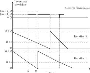
Let us investigate the system to achieve the central warehouse inventory position. As it can be seen in Figure 3, when a retailer's inventory position reaches R + s, inventory position of central warehouse is either (m + 1)Q or (m + 2)Q, considering inventory position of retailers at t (e.g. Figure 4(a) and (b)).
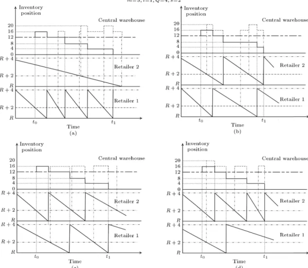
Considering m = 3, Q = 4, and s = 2, Figure 4 indicates independency of the retailer who initiates ordering Q0 and the retailer who orders Q0. For
example, consider the situation that the inventory position of Retailer 1 is R + 2 at t0 (Figure 4(a) and
(b)); in other words, Retailer 1 initiates ordering Q0.
Figure 3. The central warehouse inventory position. In this situation, based on the customers' demands with each retailer, Q0 can be shipped to Retailer 1
(Figure 4(a)) or Retailer 2 (Figure 4(b)). In the rest, for this example, we will consider the case that inventory position of Retailer 1 is equal to R + s at t0.
Furthermore, Hadley and Whitin [47] showed that at this moment, the inventory position of other retailers, i.e. Retailer 2, is uniformly distributed between R + 1 and R + Q; thus, the inventory position of the central warehouse is (m+1)Q when R+s+1 I2(t0) R+Q
with the probability of (Q s)=Q.
Let Retailer 1 order Q0; an illustration of this
system is available in Figure 5. On the other hand, we know that between t0 and t1, three batches are
ordered and inventory position of Retailer 1 equals R+1 at t1. Knowing that Retailer i can order bi batches,
so that b1+ b2 = 3, bi 08i, we want to calculate
the probability of ordering these three batches by l demands. Besides, we know that l = l1 + l2 and lr
demands cause the Retailer r to order brbatches from
the central warehouse. Considering lr= brQ + ur, we
need to obtain the probability that Retailer r receives lr demands from the total of l demands during t1 t0
and the probability that these lr demands initiate br
batches ordering, i.e. lr= brQ + ur.
The probability of distributing l demands between two retailers is l = l1+ l2 when the demand rates is
equal to
l l1
(1
2)l. Moreover, the last demand should
occur at Retailer 1. Thus, we eliminate the last demand from the combination. To do so, considering l0= l + 1,
l0
1= l1+1, and l0 = l01+l2, the probability is as follows:
1 2
l l1
1 2
l
=12
l0 1
l0 1 1
1 2
l0 1
=
l0 1
l0 1 1
1 2
l0
: (1) Let R + k0 show the inventory position of Retailer 2
Figure 4. Dierent possible combinations of retailers that cause the central warehouse to demand Q0 and the retailer
that demands Q0from the central warehouse when Iw(t0) = mQ.
at t0. For this example, we can calculate the upper
and the lower bounds of l0. To obtain the lower bound,
inventory position of Retailer 2 at t1 equals R + Q; therefore:
l0 k0+ 4(b
2 1) + 4b1+ 2: (2)
On the other hand, we know that k0 3 and b 1+
b2 = 3; thus, l0 13. It is worth mentioning that
in Figure 5(a)), the lower bound cannot be met, since b1= 3 and the lower bound is 4b1+ 2 = 14, i.e. l0= 13
is not feasible.
To obtain the upper bound, Retailer 2 inventory position should be equal to R + 1 at t1; therefore, we have:
l0 k0 1 + 4b
2+ 4b1+ 2: (3)
On the other hand, we know that k0 4 and b
1+b2= 3;
thus, l0 17.
Finally, we know that l0 = l0
1 + l2 does not
guarantee that all the conditions are held. For example,
consider l0
1= 7 and l2= 9; although 13 l0= 16 17,
the inventory position of Retailer 1 at t1 is equal to R + 4. On the other hand, consider l0
1= 14 and l2= 3;
the inventory position of Retailer 1 at t1 is equal to R + 1. However, with the probability of 1=2; k0 = 4,
which leads to a feasible solution. As a result, we need to multiply Eq. (1) by some other probability functions to obtain the probability of demanding 3 batches by these l0 demands. In other words, we should calculate
P (brQ + ur ! br), r = 1; 2, for this example. Two
illustrative computations for P (b2Q + u2 ! b2) are
presented in Figure 6.
4. Probability distribution of k
Based on Lemmas 1 and 2 proposed in [25], S0 and S
are replaced by k and R + j, respectively. Hence, the rst step for computing the probability distribution is to nd the inventory position of the central warehouse and retailers at t0. Based on the warehouse policy, inventory position of one of the retailers is R + s at
Figure 5. Possible number of batches that Retailers 1 and 2 can order when Retailer 1 causes the central warehouse to order Q0 and consume this batch.
Figure 6. Illustrative computations for P (b2Q + u2! b2)
when b2= 3 and u2= 1 or u2= 1.
this moment (without loss of generality, we name it Retailer 1). Furthermore, we know that the inventory position at the central warehouse is related to the last activities in the system. In other words, inventory
position at the central warehouse at this moment is a function of Q; m, and Retailer 2 inventory position. 4.1. The central warehouse inventory position
at t0
Inventory position for Retailer 2 is uniformly dis-tributed between R+1 and R+Q. To derive probability distribution of each system state, let I2(t0) and Ic(t0)
be the inventory positions of Retailer 2 and central warehouse at t0, respectively. As it is shown in Figure 3, at A and B, Ic (t0) is m and m + 1,
respectively:
P (i= 1; s) = P (Ic(t0) = m)
= P R + s + 1 I2(t0) R + Q
= Q s
Q ; P (i= 2; s) = P (Ic(t0) = m + 1)
= P R + 1 I2(t0) R + s
= s
Q: (4)
by Retailer r, let us introduce the following notations (note that s is one of the system parameters):
i
r;l;B;s This random variable demonstrates
the number of system batches ordered by Retailer r with l demands, when there are m + i batches at the central warehouse;
i
2;l;B;s This random variable demonstrates the
number of system batches ordered by the retailers by l demands from these retailers, when there are m + i batches at the central warehouse.
Note that, to compute i
r;l;B;s, the last customer
demand is disregarded to ensure that it is the last one among all customer demands. This demand with probability of 1
2 is assigned to Retailer B. Therefore,
for computing i
2;l;B;s, we have:
Pr(i
2;l;B;s= b) = l 1
X
k=0 b 1
X
b0=0
l k 12
l
Pr i
1;l k 1;B;s= b b0 1
Pr i
2;k;B;s= b0
: (5)
Since inventory position of each retailer is renewed for every Q customer demands, evaluating system demands will be easier using bQ + u. Hence, we can rewrite Pr(i
r;l;B;s = b), considering l = bQ + u, as
Pr(i
r;bQ+u;B;s = b). The value of this probability
depends on s, u, i, and r; i shows that there is m + i system batches at the central warehouse and s is known by system policy.
4.2. Investigating the system for s > 0 We calculate Pr(i
r;bQ+u;B;s= b) for r = 1 and r = 2,
separately.
4.2.1. Probability of ordering b batches by Retailer 1 To compute this probability, we rst investigate which retailer orders Q0. If B = 1, then at t1, the inventory
position of this retailer is R + 1. Therefore, we have: Pr i
1;bQ+u;1;s>0 = b
= 1 if B = 1;
u = s 1; b 0; 8i: (6)
On the other hand, if B 6= 1, then for this retailer, we know that Ir(t0) = R + s; we can conclude that
b0Q + s D < b0Q + Q + s surely causes b0+ 1 batch
orderings. Dening b = b0+ 1 and u = D bQ, we
have: Pr i
1;bQ+u;1;s>0 = b
= 1
r =1; B =2; s>0; s Q u < 0; b 1;
or:
r = 1; B = 2; s > 0; 0 u; b 0: (7) 4.2.2. Probability of ordering b batches by Retailer 2 Let us consider Retailer 2 when R+1 I2(t0) R+s
and B = 2. Therefore, we know that I2(t1) = R + 1.
Thus: Pr 2
2;bQ+u;2;s>0 = b
=1s;
0 u s 1; b 0: (8)
Now, consider the situation that B = 1; we know that R + 1 I2(t0) R + s and R + 1 I2(t1) R + Q.
Therefore, to order b batches by bQ + u demands, the following equation should be held:
bQ + u + I2(t0) = bQ + I2(t1) ) u
= I2(t1) I2(t0) ) 1 Q u s 1: (9)
To calculate the probability, two states are considered:
(I) 0 u s 1 or
(II) Q + 1 u 1.
In state (I), u should not exceed Ir(t0) R;
this occurs if Ir(t0) > R + u. On the other hand,
Ir(t0) is uniformly distributed over fR + 1; ; R + sg.
Therefore, the probability is as follows: Pr 2
2;bQ+u;1;s>0 = b
=s us ;
0 u s; b 0: (10)
State (II) is categorised in two subdivisions:
(II-a) s Q < u 1: In this subdivision, customer demands are equal to u + Q and the interval can be modied as s < u + Q Q. These cus-tomer demands surely trigger a retailer order, because they exceed Ir(t0). Thus, the related
probability is: Pr 2
2;bQ+u;1;s>0= b
= 1
s Q < u < 0; b 1: (11)
(II-b) Q + 1 < u s Q: As 0 < u + Q s, if these customer demands are equal to or greater than Ir(t0) R, then the retailer orders a new
batch. Thus, probability of u + Q Ir(t0) is as
follows: Pr i
r;bQ+u;B;s= b
=Q + us ;
The following probabilities can be computed with the same justication:
Pr 1
2;bQ+u;1;s>0= b
= 8 > > > > > > < > > > > > > :
1 + u
Q s s Q < u 0; b 1
1 0 u s 1; b 0
Q u
Q s s < u Q; b 0
Pr 1
2;bQ+u;2;s>0=b
=Q s1 ;
su<Q; b0: (13)
4.3. Investigating the system for s = 0 Here, Pr(i
r;bQ+u;B;s = b) is acceptable when B 1
and the last demand must be considered in order to avoid negative customer demand in the special case of B = 1 and b = 0. It is also obvious that at t0,
one batch is ordered by Retailer 1 and the central warehouse, simultaneously. Thus, Ic(t+0) = m + i and
I1(t+0) = Q.
Therefore, the probabilities of demanding b batches by Retailer r are dened as follow:
Pr 1
2;bQ+u;2;0= b
=Q1; 0 u < Q; b 0; Pr 1
2;bQ+u;2;0= b
=
(Q+u
Q Q u < 0; b 1 Q u
Q 0 u < Q; b 0
Pr 1
2;bQ+u;2;0= b
= 1; B = 2; 0 u < Q; b 0
B = 1; u = Q 1; b 0: (14)
Furthermore, for m = 0, the B batch is ordered at t0 by Retailer 1 and central warehouse, simultaneously. Thus, surely there is no need for any demand other than the mentioned one; therefore, k = 0.
5. Boundaries of customers' demand Let us introduce the following notations:
lb(i; s; m) Lower bound of customer demand for a known s, when system starts with m initial batches and Ic(t+0) = m + i;
ub(i; s; m) Upper bound of customer demand for a known s, when system starts with m initial batches and Ic(t+0) = m + i.
5.1. Lower bounds For s > 0, we know:
8 > < > :
min fI2(t0)g = R + 1 Ic(t+0) = m + 2
I1(t0) = R + s
min fI2(t0)g = R + s + 1 Ic(t+0) = m + 1
(15) Consider Ic(t+0) = m + 2; after meeting R, every
retailer should have at least Q demands to order a new batch. As a result, two batches can be ordered by s + 1 demands from each retailer and the remaining m batches are ordered by mQ demands. Furthermore, we disregard the last customer demand; therefore, we have:
lb(2; s > 0; m) = s + 1 + mQ: (16) Now, we investigate Ic(t+0) = 1 and m = 0. At least
s demands from Retailer 1 can cause ordering a new batch. Thus:
lb(1; s > 0; 0) = s: (17)
On the other hand, for m > 0, with a justication as before, the lower bound will be:
lb(1; s > 0; m > 0) = 2s + 1 + (m 1)Q: (18) We can summarise these bounds as:
lb(i; s > 0; m) =
(
s m + i = 1
(3 i)s + 1 + (m + i 2)Q m + i 2 (19) When s = 0, we know that Ic(t+0) = m and we have
the following inventory positions for retailers: (
I1(t+0) = R + Q
minfI2(t+0)g = R + 1
(20) Hence, at most one batch can be ordered by one customer demand and the remaining batches, if any, are ordered by Q customer demands. Therefore, generally, the lower bounds are:
lb(i; s; m)
= 8 > > > < > > > :
0 m = 0; s = 0
(m 1)Q + 1 m 1; s = 0
s m+i=1; s>0
5.2. Upper bounds When s > 0, we know that:
maxfIr(t0)g :
8 > < > :
maxfI2(t0)g = R + s Ic(t+0) = m + 2
I1(t0) = R + s
maxfI2(t0)g = R + Q Ic(t+0) = m + 1
(22) Consider Ic(t+0) = m + i; the most possible demand
occurs when one of the retailers has bQ+maxfIr(t0)g
R demands and the other one has b0Q+maxfI r0(t0)g
(R + 1), where b0+ b = m + i 1. Thus, for I c(t+0) =
m + 1, we have:
ub(1; s > 0; m) = s + Q 1 + mQ )
= s 1 + (m + 1)Q: (23)
And for Ic(t+0) = m + 2, we have:
ub(2; s > 0; m) = 2s 1 + (m + 1)Q: (24) Consequently, for s > 0, we obtain Eq. (25):
ub(i; s > 0; m) = is 1 + (m + 1)Q: (25) For s = 0 and m > 0, we know that:
maxIr t+0 :
( I1 t+0
= R + Q maxI2 t+0 = R + Q
(26) Thus, Eq. (27) is calculated as follows:
ub(1; 0; m > 0) = (m + 1)Q 1: (27) Finally, the only dierence between s = 0 and s > 0 is in the batch quantities. As mentioned before, for s = 0, we consider m batches instead of m + 1. Therefore, we have:
ub(i; s; m)= (
is 1+(m+1)Q s > 0
(m + 1)Q 1 s=0; m>0 (28) 6. The nal model and its optimisation
In this study, an arbitrary unit of Q0 is considered,
which can be the jth unit of Q0with probability of 1=Q.
Furthermore, this unit should wait for R + j additional demands from t+
1. Thus, we have Eq. (29) as shown
in Box I. This method is an extension of the method presented by Axsater (1990) [23] (see Appendix A).
Let us introduce the following notations based on [23]:
Gs(t) Cumulative distribution function of
Erlang (N; S), which is calculated as follows:
1
X
k=S
(t)k
k! e t= 1
S 1X k=0
(t)k
k! e t: (30)
S(t) Conditional expected cost of S(S0)
knowing that = t, which is independent of S0;
Ms The upper bound for the number of
initial batches in the central warehouse (m) for a given s with respect to the acceptable error;
ml
s The lower bound for m for a given s;
mu
s The upper bound for m for a given s.
For large values of S0, S(S0) can be
approx-imated by S(0); therefore, for an acceptable error
("), GM(L
0) < ". On the other hand, for a given
s,lb(1; s; m) = minflb(i; s; m)g8i. Thus:
T C(m; s; R)
= 8 > > > > > > > > > > > > > > > < > > > > > > > > > > > > > > > : 2 X i=1
p(i; s)X2
B=1
ub(i;s;m)X k=lb(i;s;m)
Pr i
2;k;B;s= m + i 1
0
@(k) + 1QXQ
j=1
R+j(k)
1
A s > 0
X2
B=1
ub(i;0;m)X k=lb(i;0;m)
Pr i
2;k;B;0= m 1
0
@(k) + 1QXQ
j=1
R+j(k)
1
A s = 0; m > 0
(k) + 1
Q Q P j=1 R+j(k) !
s = 0; m = 0 (29)
Ms= 8 > > > > > > > > > > > > < > > > > > > > > > > > > :
0 M = 0; s = 0
l
M 1 Q + 1
m
M > 0; s = 0 l
M s s+1
m
M 2s + 1; s > 0 l
M 2s 1 Q + 1
m
M > 2s + 1; s > 0 (31)
where, dxe is ceiling, i.e. the smallest integer greater than or equal to x. Furthermore, let the upper bound and the lower bound of R be Rl and Ru. Due to the
convexity of S(S
0) with respect to S for a known
S0, Rl and Ru can be calculated by minimization of 1
Q
PQ
j=1R+j(L0) and Q1 PQj=1R+j(0), respectively.
Finally, the lower bounds for Rl and Ru are Q and
Rl. Knowing Rland Ru, for a given s, mus and mlscan
be calculated as follows: 8 > > > < > > > : ml
s= min0mM
sfT C(m; s; Ru)g
mu
s =mlmin
smMsfT C(m; s; Rl)g
(32)
The following lemma leads to less computational ef-forts:
Lemma: To compute Ri
l(0) and Rui(0), it is enough
to compare R+1() with R+Q+1() using the convexity
attribute.
Proof: Optimal Ri
l(0) and Riu(0) are obtained by
comparing 1 Q
PQ
j=1R
i+j
i () with Q1
PQ
j=1R
i+1+j
i ().
Consider A =PQj=2R+j(); therefore:
1 Q
Q
X
j=1
R+j() = 1
Q(R+1() + A) and: 1 Q Q X j=1
R+1+j() = 1
Q(R+Q+1() + A):
Since A and 1
Q are common parameters, they can be
ignored.
7. Conclusions
In this paper, we modelled a two-level inventory system with two identical retailers that beneted from an information sharing policy. We proposed the exact model and a procedure to nd optimal solutions to
this problem. It is worth mentioning that both of them have been open questions up to now. We rst proposed an illustrative example to identify system states and provide better understanding of system behaviour in dierent situations. To resolve the complexity of the proposed problem, we divided the main problem into some easier sub-problems; then, we modelled the whole system by merging the sub-problems. Furthermore, we considered an arbitrary batch and derived probability distribution for the number of required demands to order this batch. Next, we proposed the boundaries of optimum variables and the nal model for the proposed system.
By modelling and proposing optimisation proce-dure for an easy to implement information sharing policy, this study can be used as a baseline for a deeper knowledge of how this policy works. It is worth mentioning that the simplicity of this policy, i.e. using limited parameters and information about inventory status and demand, makes it easy to implement in real-world scenarios in a way that managers have a sense of the inventory management scheme and the way it operates. Moreover, the shared information in this system is an acceptable range of information that is shared in distributer companies, i.e. inventory status and demand. Furthermore, the policy under study takes advantage of fast developing information technology in forms of information transfer infras-tructures, radio-frequency identication (RFID), and computational speed to propose an easy to implement inventory control scheme without any need to share crucial information or face data overload. The simplic-ity of this policy may be claimed to be a double-edged sword; however, considering the continuously growing arguments about information sharing disadvantages, the tendency to limit shared information in this model can be its positive aspect.
As future subjects of study, the exact model for more than two retailers for the proposed policy is still an open question. In addition, extending this problem to non-identical retailers and making the policy more exible are attractive problems to study. Moreover, considering dierent policies with limited dynamicity are other attractive subjects of study.
References
1. Forrester, J.W. \Industrial dynamics: a major break-through for decision makers", Harvard Business Re-view, 36(4), pp. 37-66 (1958).
2. Simchi-Levi, D., Kaminsky, P., and Simchi-Levi, E., Designing and Managing the Supply Chain: Concepts, Strategies, and Case Studies, The McGraw-Hill/Irwin Series in Operations and Decision Sciences, McGraw-Hill, Illinois (2003).
of information sharing in a two-level supply chain", Management Science, 46(5), pp. 626-643 (2000).
4. Raghunathan, S. and Yeh, A.B. \Beyond EDI: impact of continuous replenishment program (CRP) between a manufacturer and its retailers", Information Systems Research, 12(4), pp. 406-419 (2001).
5. Yao, Y. and Dresner, M. \The inventory value of information sharing, continuous replenishment, and vendor-managed inventory", Transportation Research Part E: Logistics and Transportation Review, 44(3), pp. 361-378 (2008).
6. Dong, Y., Dresner, M., and Yao, Y. \Beyond informa-tion sharing: An empirical analysis of vendor-managed inventory", Production and Operations Management, 23(5), pp. 817-828 (2014).
7. Cui, R., Allon, G., Bassamboo, A., and Van Mieghem, J.A. \Information sharing in supply chains: An empir-ical and theoretempir-ical valuation", Management Science, 61(11), pp. 2803-2824 (2015).
8. Chen, M.-C., Yang, T., and Yen, C.-T. \Investigating the value of information sharing in multi-echelon sup-ply chains", Quality & Quantity, 41(3), pp. 497-511 (2007).
9. Razmi, J., Rad, R.H., and Sangari, M.S. \Develop-ing a two-echelon mathematical model for a vendor-managed inventory (VMI) system", The International Journal of Advanced Manufacturing Technology, 48(5-8), pp. 773-783 (2010).
10. Li, C. \Controlling the bullwhip eect in a supply chain system with constrained information ows", Applied Mathematical Modelling, 37(4), pp. 1897-1909 (2013).
11. Cannella, S., Dominguez, R., Framinan, J.M., and Bruccoleri, M. \Insights on partial information sharing in supply chain dynamics", International Conference on Industrial Engineering and Systems Management (IESM), Seville, Spain, pp. 344-350 (2015).
12. Cannella, S., Framinan, J.M., and Barbosa-Povoa, A. \An IT-enabled supply chain model: a simula-tion study", Internasimula-tional Journal of Systems Science, 45(11), pp. 2327-2341 (2014).
13. Cannella, S., and Ciancimino, E. \Up-to-date supply chain management: The coordinated (S, R) order-up-to", In Advanced Manufacturing and Sustainable Logistics, Dangelmaier, W., Blecken, A., Delius, A., and S. Klopfer, Eds., pp. 175-185, Springer, Berlin, Germany (2010).
14. Cannella, S. \Order-up-to policies in information ex-change supply chains", Applied Mathematical Mod-elling, 38(23), pp. 5553-5561 (2014).
15. Prajogo, D. and Olhager, J. \Supply chain integration and performance: The eects of long-term relation-ships, information technology and sharing, and logis-tics integration", International Journal of Production Economics, 135(1), pp. 514-522 (2012).
16. Ganesh, M., Raghunathan, S., and Rajendran, C. \The value of information sharing in a multi-product, multi-level supply chain: Impact of product substi-tution, demand correlation, and partial information sharing", Decision Support Systems, 58, pp. 79-94 (2014).
17. Sabitha, D., Rajendran, C., Kalpakam, S., and Ziegler, H. \The value of information sharing in a serial supply chain with AR (1) demand and non-zero replenish-ment lead times", European Journal of Operational Research, 255(3), pp. 758-777 (2016).
18. Ali, M.M., Boylan, J.E., and Syntetos, A.A. \Forecast errors and inventory performance under forecast infor-mation sharing", International Journal of Forecasting, 28(4), pp. 830-841 (2012).
19. Babai, M.Z., Boylan, J.E., Syntetos, A.A., and Ali, M.M. \Reduction of the value of information sharing as demand becomes strongly auto-correlated", Inter-national Journal of Production Economics, 181, pp. 130-135 (2016).
20. Trapero, J.R., Kourentzes, N., and Fildes, R. \Impact of information exchange on supplier forecasting perfor-mance", Omega, 40(6), pp. 738-747 (2012).
21. Cannella, S., Lopez-Campos, M., Dominguez, R., Ashayeri, J., and Miranda, P.A. \A simulation model of a coordinated decentralized supply chain", Inter-national Transactions in Operational Research, 22(4), pp. 735-756 (2015).
22. Li, X. and Wang, Q. \Coordination mechanisms of sup-ply chain systems", European Journal of Operational Research, 179(1), pp. 1-16 (2007).
23. Axsater, S. \Simple solution procedures for a class of two-echelon inventory problems", Operations Re-search, 38(1), pp. 64-69 (1990).
24. Axsater, S. \Exact and approximate evaluation of batch-ordering policies for two-level inventory sys-tems", Operations Research, 41(4), pp. 777-785 (1993).
25. Forsberg, R. \Optimization of order-up-to-S policies for two-level inventory systems with compound Poisson demand", European Journal of Operational Research, 81(1), pp. 143-153 (1995).
26. Forsberg, R. \Exact evaluation of (R, Q)-policies for two-level inventory systems with Poisson demand", European Journal of Operational Research, 96(1), pp. 130-138 (1997).
27. Axsater, S. \Exact analysis of continuous review (R,Q) policies in two-echelon inventory systems with com-pound Poisson demand", Operations Research, 48(5), pp. 686-696 (2000).
28. Simchi-Levi, D. and Zhao, Y. \Three generic meth-ods for evaluating stochastic multi-echelon inventory systems", Working Paper, Massachusetts Institute of Technology, Cambridge (2007).
29. Simchi-Levi, D. and Zhao, Y. \Performance evaluation of stochastic multi-echelon inventory systems: a sur-vey", Advances in Operations Research, 2012, Article ID: 126254, 34 pages (2012).
https://doi.org/10.1155/2012/126254
30. Chen, F. and Zheng, Y.-S. \Evaluating echelon stock (R, nQ) policies in serial production/inventory sys-tems with stochastic demand", Management Science, 40(10), pp. 1262-1275 (1994).
31. Chen, F. and Zheng, Y.-S. \Near-optimal echelon-stock (R, nQ) policies in multistage serial systems", Operations Research, 46(4), pp. 592-602 (1998).
32. Axsater, S. and Rosling, K. \Notes: Installation vs. echelon stock policies for multilevel inventory control", Management Science, 39(10), pp. 1274-1280 (1993).
33. Moinzadeh, K. \A multi-echelon inventory system with information exchange", Management Science, 48(3), pp. 414-426 (2002).
34. Haji, R. and Sajadifar, S.M. \Deriving the exact cost function for a two-level inventory system with infor-mation sharing", Journal of Industrial and Systems Engineering, 2(1), pp. 41-50 (2008).
35. Sajadifar, S.M. and Haji, R. \Optimal solution for a two-level inventory system with information exchange leading to a more computationally ecient search", Applied Mathematics and Computation, 189(2), pp. 1341-1349 (2007).
36. Axsater, S. and Marklund, J. \Optimal position-based warehouse ordering in divergent two-echelon inventory systems", Operations Research, 56(4), pp. 976-991 (2008).
37. Svoronos, A. and Zipkin, P. \Estimating the perfor-mance of multi-level inventory systems", Operations Research, 36(1), pp. 57-72 (1988).
38. Deuermeyer, B.L., and Schwarz, L.B., A Model for the Analysis of System Service Level in Warehouse-Retailer Distribution Systems: the Identical Warehouse-Retailer Case, Purdue University (1981).
39. Cachon, G.P. and Fisher, M. \Supply chain inventory management and the value of shared information", Management Science, 46(8), pp. 1032-1048 (2000).
40. Gurbuz, M.C., Moinzadeh, K., and Zhou, Y.P. \Coordinated replenishment strategies in inven-tory/distribution systems", Management Science, 53(2), pp. 293-307 (2007).
41. Wang, Q., Chay, Y., and Wu, Z. \A simple coor-dination strategy for a decentralized supply chain", Working Paper, Nanyang Business School, Nanyang Technological University, Singapore (2006).
42. Klastorin, T.D., Moinzadeh, K., and Son, J. \Coor-dinating orders in supply chains through price dis-counts", IIE Transactions, 34(8), pp. 679-689 (2002).
43. Haji, R. and Haji, A. \One-for-one period policy and its optimal solution", Journal of Industrial and Systems Engineering, 1(2), pp. 200-217 (2007).
44. Kurt Salmon Associates, Inc., Ecient Consumer Response: Enhancing Consumer Value in the Grocery Industry, Research Department Food Marketing Insti-tute, Washington, Dc (1993).
45. Kurt Salmon Associates, Inc., Quick Response: Meet-ing Customer Need, Kurt Salmon Associates, Atlanta, GA (1997).
46. Stalk, G., Evans, P., and Shulman, L.E. \Competing on capabilities: The new rules of corporate strategy", Harvard Business Review, 70(2), pp. 57-69 (1991).
47. Hadley, G. and Whitin, T.M., Analysis of Inventory Systems, Prentice Hall, Englewood, Clis, NJ (1963).
Appendix A
In this part, a summary of [23] cost functions is proposed.
0 is demand intensity at the central warehouse
(PNi=1i). Note that in our paper, 0is equal to N.
The average holding cost in the central warehouse (S0) is:
(S0)=e 0L0h0 0
SX0 1
k=0
(S0 k)
k! (0L0)k; S0>0:(A.1) Or equally:
(S0) =h0S0 0 :
1 GS0+1
0 (L0)
h0L0
1 GS0
0 (L0)
; S0> 0: (A.2)
For S0 0, we have:
(S0) = 0; S0 0: (A.3)
The unit cost at retailer i for a given delay equal to t at the warehouse is:
Si
i (t) =e i(Li+t)hi+i i
SXi 1
k=0
(Si k)
k! ki(Li+t)k
+ i
Li+ t Si i
: (A.4)
For Si 0, average holding and shortage cost in retailer
i, Si
i (S0), is:
Si
i (S0) =GS00(L0)iL0 GS00+1(L0)iLS0 0
+ i
Li LSi
i
; Si 0; S0> 0;
(A.5) and:
Si
i (S0) = i
Li+ L0 SLi i
S0
L0
;
Si 0; S0 0: (A.6)
For Si > 0, it is possible to obtain the following
recursive equation: Si
i (S0 1) = i 0
Si 1
i (S0) +0 i 0
Si
i (S0)
+ i 0
1 GS0
0 (L0) iSi(0) Sii 1(0)
;
S0> 0: (A.7)
For S0 0, we have:
Si
i (S0 1) = i 0
Si 1
i (S0) +0 i 0
Si
i (S0);
S0 0: (A.8)
0
i(S0) can be obtained by Eqs. (A.5) and (A.6).
Finally, for suciently large values of S0, the
delay at warehouse is equal to 0; thus, we have: Si
i (S0) Sii(0): (A.9)
This approximation is asymptotically exact. To deter-mine an initial large value of S0, let the probability that
the warehouse can deliver without a delay be smaller than ":
GS0
0 (L0) < "; (A.10)
where " is a small positive number.
Biographies
Amir Hosein Afshar Sedigh is currently a PhD can-didatein Information Science at University of Otago, Dunedin, New Zealand. He received a BSc degree in Industrial Engineering from Qazvin Islamic Azad University, Qazvin, Iran. Thereafter, he received his MSc degree in Industrial Engineering from Sharif University of Technology, Tehran, Iran. His research interests include supply chain management, inventory control, and queuing theory.
Rasoul Haji is currently a Professor of Industrial Engineering at Sharif University of Technology in Tehran, Iran. He received a BSc degree from Uni-versity of Tehran in Chemical Engineering in 1964. In 1967, he received his MSc degree and then, in 1970, his PhD degree both in Industrial Engineer-ing from the University of California-Berkeley. He is recognized as a co-founder of a fundamental and important relation in queuing theory known as \Distri-butional Little's Law". His research interests include inventory control, stochastic processes, and queuing theory.
Seyed Mehdi Sajadifar is currently an Assistant Professor of Industrial Engineering at University of Science and Culture in Tehran, Iran. He received a BSc degree from Sharif University of Technology in Indus-trial Engineering in 1995. In 1997, he received his MSc degree and then, in 2008, after experiencing 5 years of academic teaching, his PhD degree in Industrial Engineering both from Sharif University of Technology. His research interests include inventory management, supply chain management, and operations research.