VOLUME 37, ARTICLE 34, PAGES 1049
,
1080
PUBLISHED 13 OCTOBER 2017
http://www.demographic-research.org/Volumes/Vol37/34/ DOI: 10.4054/DemRes.2017.37.34
Research Article
The impact of kin availability, parental
religiosity, and nativity on fertility differentials
in the late 19
th-century United States
J. David Hacker
Evan Roberts
This publication is part of the Special Collection on “The Power of the Family,” organized by Guest Editors Hilde A.J. Bras and Rebecca Sear.
© 2017 J. David Hacker & Evan Roberts.
This open-access work is published under the terms of the Creative Commons Attribution NonCommercial License 2.0 Germany, which permits use, reproduction & distribution in any medium for non-commercial purposes, provided the original author(s) and source are given credit.
1 Introduction 1050
2 Prior research on the US fertility transition 1051
3 Measurement of kin proximity 1052
4 Measurement of nativity and religiosity 1060
5 Methods and results 1063
5.1 Descriptive results 1064
6 Poisson analysis 1067
7 Conclusion 1072
8 Acknowledgments 1073
The impact of kin availability, parental religiosity, and nativity on
fertility differentials in the late 19
th-century United States
J. David Hacker1 Evan Roberts2
Abstract
METHODS
Most quantitative research on fertility decline in the United States ignores the potential impact of cultural and familial factors. We rely on new complete-count data from the 1880 US census to construct couple-level measures of nativity/ethnicity, religiosity, and kin availability. We include these measures with a comprehensive set of demographic, economic, and contextual variables in Poisson regression models of net marital fertility to assess their relative importance. We construct models with and without area-fixed effects to control for unobserved heterogeneity.
CONTRIBUTION
All else being equal, we find a strong impact of nativity on recent net marital fertility. Fertility differentials among second-generation couples relative to the native-born white population of native parentage were in most cases less than half of the differential observed among first-generation immigrants, suggesting greater assimilation to native-born American childbearing norms. Our measures of parental religiosity and familial propinquity indicate a more modest impact on marital fertility. Couples who chose biblical names for their children had approximately 3% more children than couples relying on secular names, while the presence of a potential mother-in-law in a nearby household was associated with 2% more children. Overall, our results demonstrate the need for more inclusive models of fertility behavior that include cultural and familial covariates.
1. Introduction
Total fertility in the United States fell from 7.0 in 1835, one of the highest rates in the world, to 2.1 in 1935, one of the lowest rates (Coale and Zelnik 1963; Hacker 2003). Although most researchers emphasize the causal role of economic modernization (e.g., Jones and Tertilt 2008), cultural and familial factors affected the timing and pace of the decline. Fertility differentials were large between native-born and foreign-born women and among women residing in areas dominated by liberal, evangelical, and conservative churches, even after controlling for economic and demographic variables (Hareven and Vinvoskis 1975; Morgan, Watkins, and Ewbank 1994; Haines and Hacker 2011). Parents relying on biblical names for the children had more children than parents relying on secular names, suggesting an association between parental religiosity and marital fertility (Hacker 1999, 2016). There is also evidence of a significant intergenerational link between parents’ and children’s fertility during the decline, with men and women from large families of origin tending to have more children than men and women from small families (Jennings, Sullivan, and Hacker 2012). Couples living in New England had persistently lower fertility throughout the decline, and the region continues to exhibit unique demographic behaviors today, more in line with the ‘low-low’ fertility rates in parts of Europe than with the rest of the United States (Lesthaeghe and Neidert 2006; Hacker 2016). These differentials suggest the need for a better understanding of the contribution of cultural and familial influences in the US fertility transition.
2. Prior research on the US fertility transition
Quantitative research on the US fertility transition has emphasized economic factors. Because US fertility decline began when the nation was still overwhelmingly rural, researchers have focused their investigations on the possible role of changes in the agricultural economy on reproductive behavior. Differentials in child-woman ratios, which are available at the county level between 1800 and 1860, have been associated with differentials in the availability of land for farming, the price of local farms, and other measures of the agricultural economy, suggesting that parents adapted to declining agricultural opportunities by limiting their fertility (Yasuba 1962; Forster and Tucker 1972; Easterlin 1976; Vinovskis 1976; Easterlin, Alter, and Condran 1978; Smith 1987; Carter, Ransom, and Sutch 2004; Haines and Hacker 2011). Research on the post-1860 period has also emphasized couples’ economic motivations to reduce fertility but has stressed the contributing roles of urbanization, industrialization, higher incomes, and compulsory schooling (Guest 1981; Guest and Tolnay 1983; Wanamaker 2012). In their recent analysis of children-ever-born data in the 1900, 1910, and 1940– 1990 IPUMS samples, Jones and Tertilt (2008) found a consistent negative relationship between fertility and ‘occupational income’ from the earliest observable birth cohort in 1826. Other researchers have highlighted large and increasing fertility differentials between women married to men in farm and nonfarm occupations, especially between women married to farmers and women married to men in professional, sales, and managerial occupations (Stevenson 1920; Haines 1992; Dribe, Hacker, and Scalone 2014).
limitation techniques (Parkerson and Parkerson 1988; Leasure 1982; Smith 1987; Hacker 1999; Haines and Hacker 2011).
American historical demographers have paid little attention to the role of kin in fertility decisions. A recent study based on the Utah Historical Database, however, found higher fertility among women with living mothers and mothers-in-law during the fertility transition (Jennings, Sullivan, and Hacker 2012). The finding is consistent with research in evolutionary anthropology that stresses the importance of economic and physical assistance from relatives, particularly postmenopausal grandmothers, in the rearing of human children. When fecund couples reside far from their own parents, the labor and economic burden of child rearing falls more on the child-bearing couple. Couples without significant help are more likely to reduce family size, while couples surrounded by kin networks are inclined to have more children (Hrdy 2009; Hawkes, O’Connell, and Blurton Jones 1989; Turke 1988; Sear and Coall 2011). Proximity to kin may also induce higher levels of fertility through an effect called ‘kin priming’ (Mathews and Sear 2013; Newson et al. 2005). People living close to kin have higher fertility because social interactions with their kin influence them – at least subconsciously – to have more children. Loosely speaking, ‘kin priming’ is the effect of your parents asking you when you are going to have another baby. Although these two effects are theoretically distinct, they operate in mostly the same direction, with increasing proximity leading to higher fertility. Sears and Coall’s useful survey of 39 studies (2011) indicates that paternal kin have a more consistent pronatal impact on fertility than maternal kin, consistent with the evidence that maternal kin may act at times to protect women from maternal depletion – the negative impact on a woman’s own health of having additional children.
3. Measurement of kin proximity
The measurement of kin proximity is a core challenge of this literature. We observe that declining fertility in 19th-century Europe and North America was coincident with high levels of domestic and international migration, and that migration was more often across greater distances in the 19th century than it had been in the 18th century. But this level of aggregation is too coarse to establish links between kin proximity and fertility decisions. What matters for individual fertility decisions is not overall migration rates, but the migration, or not, of your relatives.
2003). More generally, this is a problem of measuring social networks and relationships. Censuses can tell us when people reside together and often describe their relationship to each other. Institutional records, such as school rolls or church membership lists, can be used to place people in the same social milieu. But these are fairly selective sources, and capture only relationships within formal organizations. Measuring social networks of any kind often requires direct questions to subjects about who they are related to in particular ways, including kin.
Thus kin proximity has to be measured by direct questions on the distance to defined categories of family members, such as parents and siblings. Ernest Burgess’ pioneering and influential surveys of marriage in the 1930s may have been the first to include questions of this nature. The questionnaires for Burgess’s first study – the ‘526 study’ in the early 1930s – asked explicitly how far couples lived from the parents of the wife and the husband (Burgess and Cottrell 1939). Although the question was repeated in his larger (‘Over 1,000’) longitudinal survey of engaged and married couples beginning in the late 1930s, little use of the variable was made in the main publications resulting from these studies (Burgess and Wallin 1953). Geographical proximity to parents and in-laws was regarded as an ‘intruding’ variable in the more important analysis of measures of emotional closeness (Wallin 1954). Subsequent studies by other sociologists and demographers in the 1950s also collected measures of physical proximity but made perfunctory use of it (Landis 1960; Wallin 1954). A precedent for collecting measures of kin proximity had been established, and major surveys of family relationships in several countries now include questions on geographic proximity of kin (Sear and Coall 2011). For example, in the United States, surveys such as the Health and Retirement Survey include questions on kin proximity. Research with this data has found that kin proximity is an important influence on adults’ residential moves. Kin who live close by are a brake on moving, and many moves are motivated by the imperative of reducing distance between adult children and parents (Spring et al. 2017). Yet much of this data pertains to families in the recent past, after the peak of the baby boom, or to lower-income families in modern societies. We know little about the effects of kin proximity in North America and Western Europe during the early stages of the demographic transition.
they often lack detailed socioeconomic and residential data. The Utah Historical Database, constructed from genealogical information captured for ancestors of the Church of Latter Day Saints, for example – which was used by Jennings, Sullivan, and Hacker to examine the potential impact of mothers and mothers-in-law on women’s fertility decisions (2012) – lacks detailed residence information. The positive impact of mothers and mothers-in-law on fertility was estimated from their vital status (living or dead), not their physical proximity to their children. Sherry Olson traced forward 19th -century families in Montreal from the 1881 to 1901 census. With familial relationships taken from 1881, she was able to see how closely parents and adult children resided in 1901. Adult children within Montreal lived close to their parents, with three-quarters living within two kilometers, suggesting that family ties were important in deciding where to live (Olson 2015).
In this paper, we take advantage of the recent availability of complete-count census data to measure the proximity of potential kin to married couples and study its effects on fertility. Complete-count census data with identifying information (surnames) has become publicly available to scholars in the past decade (Ruggles 2014). Scholars have used this data to study related topics such as household composition (Ruggles 2009) and fertility (Dribe, Hacker, and Scalone 2014), taking advantage of the detailed information on within-household relationships in these datasets.3
We can infer the presence of potential kin in nearby households by using surnames, parental birthplaces, and ages, and by taking advantage of the way in which the census was taken. In the United States, at least, the census collected information from households in essentially sequential order (Grigoryeva and Ruef 2015; Logan and Parman 2017). This sequence is maintained in the data through the variable ‘serial,’ which identifies unique households within a census year. (Within-household individuals are further identified by an index called ‘pernum.’) Serial numbers respect the sequence of the original enumeration that was constructed by 1) enumerating households in geographic sequence, and 2) numbering enumeration sheets in a manner that maintained this geographic order. However, not all sequential serial numbers are adjacent. ‘Serial’ maintains its sequence from state to state, and it is highly unlikely – though not absolutely impossible – that serialt is a real neighbor of serialt+1 whent andt+1 are in different states, as relatively few state borders are found in settled areas, particularly in the 19th century. Thus we must look for smaller geographic units in which to sort our serial numbers and find adjacent houses.
Enumeration districts formed the basic administrative geography of the census, within which households were canvassed sequentially. In the 1880 census from which we draw the data for this paper, there were 11,349 enumeration districts for a population of just over 50 million. Enumeration districts ranged in population size from
10 to 30,000. The largest enumeration districts were found in large, dense cities such as Chicago, New York, St. Louis, and Cleveland, where they were geographically small and contiguous. Although the local administration of the census in the United States was problematic because it led to greater variability in enumeration practices, it did allow local officials to construct enumeration districts that conformed to areas recognized by the people they were enumerating. Where the borders are known, they run down major roads, or along barriers such as geographic features or railroads. In rural areas enumeration districts also conformed to recognized neighborhoods (Logan and Parman 2017). For the vast majority of households within an enumeration district, households with sequential serial numbers in the data are, in fact, adjacent in physical space, and if not adjacent very close.
We take advantage of this property of the complete-count data and individuals’ reported surnames, birthplaces, and ages to measure couples’ potential kin in nearby houses. In our initial analysis, we followed the existing literature, using neighbors in complete-count census data, and analyzed only the two adjacent households, focusing on identifying the presence of a potential mother-in-law for all currently married women of childbearing age (Grigoryeva and Ruef 2015; Logan and Parman 2017). We extend prior scholarship by examining a wider window around the focal household to identify additional potential mothers-in-law, although the likelihood of finding one declined with each household. Ultimately, as discussed in more detail below, we limited our search to ten ‘nearby’ households, defined as the five households on either side of each focal woman.
density of kin networks in towns and cities. With these explanations of the strengths of our measure of geographic proximity (‘nearby’ households in the data are geographically close) and the limitations (borders of districts are not known and we may miss some potential kin living nearby), we turn to discussion of measuring actual kin within the household and potential mothers-in-law outside it.
The census began directly enumerating relationships within households for the first time in the 1880 census. The version of the 1880 census that we use in this article comes from the North Atlantic Population Project, for which the original records were transcribed by the Church of Jesus Christ of Latter Day Saints (LDS). In the process of transcribing the complete 1880 census, the LDS removed information on nonfamily relationships within the household (Minnesota Population Center 2015; Roberts et al. 2003). Thus all people with nonfamilial relationships, such as boarders and lodgers, receive the same relationship code in the data. However, our analysis focuses on currently married women age 20–49 living with their spouse (henceforth, the ‘study population’), 99% of whom had a familial relationship to the head of household. Thus we can reliably determine within-household kin for nearly the entire study population. After restricting the universe to women with no missing information, our study population includes 5,379,539 women.
To measure kin and other sources of support for child rearing within the household, we construct indicators for having a coresident mother-in-law (3.3% of women in the study population) or a coresident mother (2.9%). We also measure the number of other females 11 years old or older, both kin and nonkin, living in the household. Almost half (45.3%) of currently married women age 20–49 had coresident females in the household, and 38.6% of women had a coresident female family member 11 or older (who was not their mother or mother-in-law). Women with a coresident mother or mother-in-law were more likely to have other female relatives living with them. These measures of household composition are standard in the fertility literature when household censuses are used.
(+/- 5 households from the focal household), increased the number of potential mothers-in-law by a factor of 3, to 6.9%. Given the much greater programming challenges of larger search windows and the increasing possibility of false positives, we decided to limit our window to the nearest ten households.
Although we label our variable ‘potential mothers-in-law,’ it is likely that some of the identified ‘mothers-in-law’ are aunts-in-law, significantly older sisters-in-law, and other ever-married female in-laws. It was therefore possible for focal women to have more than one potential mother-in-law. Among the approximately 479,000 women with a potential mother-in-law in nearby houses, however, 437,000 had just one potential mother-in-law. Although a higher number of potential mothers-in-law had meaning, we decided to treat the measure as a dichotomous indicator. The variable was set to zero for focal women with a coresident mother-in-law and one for women with one or more potential mothers-in law. We excluded from our construction of neighboring houses any group quarters, such as prisons or hospitals or poor farms, and limited our search to the nearest ten regular households.
An outline of how we proceeded programmatically may be helpful. Previous work that uses the complete-count census to identify the characteristics of neighbors has focused on racial composition of households in an era in which households themselves were nearly universally racially homogeneous (Grigoryeva and Ruef 2015; Logan and Parman 2017). When households are homogeneous on some social dimension – such as race – their characteristics can be summarized easily by collapsing the dataset to a single observation per household. Looking forward or back one household to find the characteristics of neighbors is then a matter of searching forward or back one observation and comparing the characteristic.
In general this is not possible in our situation for several reasons. First, in some households there may be multiple women whose potential kin we are interested in finding. Indeed, 16% of women in our study population resided in a household with two or more women age 20–49. Even when these women come from the same family, their potential mothers (in-law) are not necessarily the same people. This is the case in living situations such as a woman residing with her own mother, or two married couples sharing a household (e.g., married brothers farming together).
than the prior question of multiple fertile women in a household: 97% of women in the study population belonged to the first family group in the household.
Finally, households are of different sizes, and the women whose fertility we are interested in measuring necessarily appear at variable places in the household. Similarly, the potential mothers or mothers-in-law appear at different points in the neighboring households. For all the reasons just adduced, we cannot summarize the potential kin that we are interested in measuring at a household level, and we cannot prespecify the number of adjacent individual observations in the data to search for potential kin.
Table 1: Example of data processing
Actual
serial Modifiedserial pernum Relationship tohousehold head Neighborindex Last name First name Age Sex
1 1 1 Head 0 ELLIS THADDEUS 48 Male
1 1 2 Spouse 0 ELLIS CAROLINE 46 Female
1 1 3 Child 0 ELLIS THADDEUS F. 23 Male
1 1 4 Child 0 ELLIS EDWIN P. 22 Male
1 1 5 Child 0 ELLIS WILLIAM W. 19 Male
1 1 6 Child 0 ELLIS JULIA A. 17 Female
1 1 7 Child 0 ELLIS GILBERT E. 14 Male
1 1 8 Child 0 ELLIS ANGIE B. 9 Female
2 1 1 Neighbor 1 BAKER MARY C. 54 Female
2 1 2 Neighbor 1 BAKER LAURA E. 29 Female
2 1 3 Neighbor 1 BAKER FANNIE C. 22 Female
2 1 4 Neighbor 1 BAKER ELEANOR J. 20 Female
2 1 5 Neighbor 1 BAKER LYDIA J. 17 Female
1 2 1 Neighbor –1 ELLIS THADDEUS 48 Male
1 2 2 Neighbor –1 ELLIS CAROLINE 46 Female
1 2 3 Neighbor –1 ELLIS THADDEUS F. 23 Male
1 2 4 Neighbor –1 ELLIS EDWIN P. 22 Male
1 2 5 Neighbor –1 ELLIS WILLIAM W. 19 Male
1 2 6 Neighbor –1 ELLIS JULIA A. 17 Female
1 2 7 Neighbor –1 ELLIS GILBERT E. 14 Male
1 2 8 Neighbor –1 ELLIS ANGIE B. 9 Female
2 2 1 Head 0 BAKER MARY C. 54 Female
2 2 2 Child 0 BAKER LAURA E. 29 Female
2 2 3 Child 0 BAKER FANNIE C. 22 Female
2 2 4 Child 0 BAKER ELEANOR J. 20 Female
2 2 5 Child 0 BAKER LYDIA J. 17 Female
3 2 1 Neighbor 1 BAKER HENRY E. 30 Male
3 2 2 Neighbor 1 BAKER ALMIRA C. 28 Female
3 2 3 Neighbor 1 BAKER LYDIA A. 7 Female
3 2 4 Neighbor 1 BAKER – 2 Female
2 3 1 Neighbor –1 BAKER MARY C. 54 Female
2 3 2 Neighbor –1 BAKER LAURA E. 29 Female
2 3 3 Neighbor –1 BAKER FANNIE C. 22 Female
2 3 4 Neighbor –1 BAKER ELEANOR J. 20 Female
2 3 5 Neighbor –1 BAKER LYDIA J. 17 Female
3 3 1 Head 0 BAKER HENRY E. 30 Male
3 3 2 Spouse 0 BAKER ALMIRA C. 28 Female
3 3 3 Child 0 BAKER LYDIA A. 7 Female
3 3 4 Child 0 BAKER – 2 Female
4 3 1 Neighbor 1 ROGERS DEMIRA 39 Male
4 3 2 Neighbor 1 ROGERS MELISSA J. 38 Female
4 3 3 Neighbor 1 ROGERS FRED L. 14 Male
4 3 4 Neighbor 1 ROGERS FLORENCE E. 4 Female
Nearly every household in the data is treated in the same way as this example, with the search window expanded to plus or minus five households. Households appear once as the focal household (neighbor index = 0), five times as the neighbor before (or above) the focal household in the database (neighbor index = –1 to –5), and five times as the neighbor after (or below) the focal household (neighbor index = 1 to 5). We modify this procedure for households within five households of the beginning or end of the enumeration district. In these cases we search for kin among the ten closest households, which are the ten households below the first household in the enumeration district, one household before and nine households after the second household, etc. to the ten households above the last household in the district. We implement this strategy in Stata. Stata holds the data in memory, which allows us to easily compute measures of potential kin within the group identified by the modified serial number (the focal household augmented by its neighbors). As noted above there can be multiple women within a household for whom we are interested in finding potential kin, and the criteria for those kin may differ. Within a household the number of women we are interested in finding kin for is small, so we run a loop for each target woman, marking neighbors in the augmented household as potential kin or not. Finally, for each target woman we sum the number of potential kin of each category.
4. Measurement of nativity and religiosity
Fertility differentials by nativity were first highlighted by 19th-century observers. In 1877, for example, Dr. Nathan Allen estimated that the birth rate among the foreign born in New England was twice that of the native born – a result, he believed, of a desire for a higher standard of living among the native born and, perhaps, physiological degeneration among native-born men and women related to changes in work and education (Allen 1877).
high fertility regimes widened fertility differentials in the early 20th century (King and Ruggles 1990; Morgan, Watkins, and Ewbank 1992; Gjerde and McCants 1995; Reher 1998; MacNamara 2014).
Although the acquisition of English and occupational and social mobility by foreign-born couples was associated with lower marital fertility rates, nativity remained a significant correlate of marital fertility rates. Morgan, Watkins, and Ewbank (1994) found substantial marital fertility differentials by nativity in 1910, even after controlling for age, occupation, residence, duration in the United States, and ability to speak English. Second-generation couples (native born of foreign-born parents) typically achieved fertility levels between that of native-born whites and first-generation immigrants, suggesting a slow process of acculturation to American norms spanning several generations.
Prior research has also confirmed the existence of substantial differentials in fertility by nativity in the 19th century. Most studies, however, are based on aggregate child-woman ratios, include few other explanatory variables, and do not estimate the impact of generation on fertility. Our analysis models marital fertility at the level of individual couples, includes a diverse set of economic and cultural covariates, and estimates first and second-generation fertility relative to that of native born couples of native parentage. Because the nativity of wives and husbands were highly correlated, we treat nativity as a couple-level measure.4 If only one partner was native born, the nativity of the foreign-born partner was used. If both partners were foreign born but with different nativities, we relied on the wife’s nativity. We consider 15 different nativities (first-generation Irish, German, British, Canadian, Scandinavian, French, and Other foreign born; second-generation Irish, German, British, Canadian, Scandinavian, French, and Other foreign-born parents; and native born of native parents). Second-generation couples were defined a couples having one or more parents who were foreign born. When husbands and wives had parents with different nativities, we identified the couples’ second-generation nativity as the mother’s nativity over the father’s nativity, and the nativity of the wife’s mother and father over the husband’s mother and father. All else being equal, it was expected that foreign-born couples originating from countries that had yet to experience the onset of the fertility transition (all countries except France) would be less willing than native born couples to limit their fertility.
Nativity is highly correlated with the availability of potential kin. First-generation couples probably had few parents in the United States. Cultural norms about living with parents may have varied among groups, including among second-generation immigrants. Our data indicates that native-born couples of native parentage (NBNP)
4 94% of native-born wives had native-born husbands, while 90% of foreign-born wives had foreign-born
were 3.7 times more likely to have a potential mother-in-law residing within ten households than all foreign-born couples combined, 65% more likely to have a coresident mother-in-law, and 19% more likely to have a coresident mother. Differences between NBNP couples and second-generation couples were more modest but still significant. NBNP couples had about 37% more potential mothers-in-law nearby, 7% more coresident mothers-in-law, and 10% fewer coresident mothers than second-generation couples combined. To account for these differences, we interacted all nativity and kin availability variables in our models.
Our measurement of parental religiosity was less direct. Unfortunately, systematic information on religious affiliation, church attendance, and religiosity is not available until the mid-20th century. To overcome data limitations – which also affect most other countries experiencing fertility declines in the 19th century – the editors of a recent book on religiosity and fertility decline urged investigators to “be innovative in their research, and where possible to use indirect indicators for the relevant [religious] dimensions” (van Poppel and Derosas 2006: 10–11). In the 19th-century United States, where parents were free to name their children without church or state restrictions, one such indirect indictor of religiosity is parents’ choice of biblical or nonbiblical names for their children (Hacker 1999, 2016). Large shifts in the name pool over the course of the 19th century indicate that parents took advantage of this freedom. Between 1780 and 1880, the percentage of white males given a name found in the Bible fell from 67% to
under 30%. 19th-century observers bemoaned the trend, associating it with religious
declension. In a book on manners published in 1873, for example, Robert Tomes observed that while the pious continued to “turn to the Bible for a choice, and affix to their children, with an almost superstitious hope of sanctification, the names of some patriarch, saint, or apostle,” the nonpious were more apt to borrow “the name of a favorite hero or heroine” from a novel or a name associated with patriotic causes, such as Washington and Franklin (cited in Hacker 1999).
native parentage to limit the possible bias of including immigrant groups with different naming practices.
5. Methods and results
We rely on Poisson regression of the number of own children less than age 5 as the dependent variable. Because we lack information about children who may have died in the five years prior to the census, the variable is more precisely a measure of net marital fertility or marital reproduction.5 Four models are constructed. Model 1 is a Poisson regression of all currently married women age 20–49 with spouses present. After restricting the universe to women with nonmissing information, our study population includes 5,379,539 women. Model 2 employs the same universe and variables but applies fixed effects at the State Economic Area (SEA) level (an aggregation of two or more contiguous counties identified by the 1950 census as sharing similar economic characteristics). In 1880 there are 423 SEAs containing an average of about 12,800 child-bearing women. The fixed effects control for unobserved heterogeneity across SEAs. Models 3 and 4 are based on the same specifications of models 1 and 2 but with the universe limited to native-born couples with native-born parents, which reduces the study population to 3,092,056 women. We focus our discussion on model 2.
Independent variables were sorted into five major groups: variables associated with availability of potential help rearing children (coresidence of mother, coresidence of mother-in-law, number of coresiding older females, and the presence of a potential mother-in-law living in ten nearby households), variables primarily associated with economic ‘readiness,’ variables primarily associated with cultural ‘willingness,’ other covariates, and demographic control variables. Readiness variables included women’s labor force participation, spouse’s occupation, the average value of farms in couples’ county of residence, and the proportion of children age 8–14 in the county in school. Couples living on farms, for example, where children could assist in farm chores and were less an economic burden, might not perceive an economic benefit from lowering their fertility and were therefore less ‘ready’ to adopt birth control methods. Cultural ‘willingness’ variables included the proportion of children biblically named, race, and couples’ nativity and generation. Other covariates and demographic control variables included population size of town or city, women’s age, age differential from spouse,
5 With the possible exception of the urban-rural differentials discussed below, differentials in the number of
and prior fertility, defined as the number of living children in the household age 5 and above. The latter variable serves as a control for the focal woman’s fecundity.
A few of our independent variables were modestly correlated. The presence of a focal woman’s mother in the household, for example, was negatively correlated with the presence of a mother-in-law (r = –0.02) and positively correlated with the number of other females over age 10 in the household (r = 0.03). Unsurprisingly, the number of females age 11 and older in the household available for childrearing assistance was strongly correlated with a woman’s prior fertility (r = 0.54). Although regression coefficients are unbiased by multicollinearity, standard errors are inflated, which can cause coefficients to be estimated less accurately when the number of cases is small. However, because we have complete population data, there is no sampling error, and so standard errors are not affected by multicollinearity (Goldberger 1991: 245–251).
5.1 Descriptive results
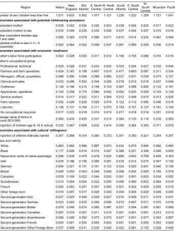
Table 2: Means of variables in regression models by census division
Region NationEnglandNew AtlanticMid E. NorthCentralW. NorthCentral AtlanticSouth E. SouthCentral SouthW. Central
Mountain Pacific
Number of own children less than five 1.071 0.833 0.952 1.017 1.121 1.226 1.222 1.258 1.121 1.041 Covariates associated with potential childrearing assistance
Coresident mother 0.029 0.042 0.034 0.026 0.023 0.029 0.026 0.025 0.017 0.023 Coresident mother-in-law 0.033 0.048 0.035 0.030 0.026 0.037 0.034 0.027 0.015 0.016 Other coresident females age
11 and older 0.585 0.583 0.579 0.586 0.571 0.615 0.614 0.534 0.467 0.594 Potential mother-in-law in +/– 5
households 0.063 0.064 0.052 0.059 0.047 0.091 0.090 0.055 0.056 0.019 Covariates associated with economic ‘readiness’
Mother’s labor force participation 0.043 0.028 0.020 0.011 0.012 0.106 0.105 0.086 0.016 0.016 Father’s occupational group
Professional, technical 0.029 0.028 0.031 0.033 0.032 0.023 0.024 0.027 0.032 0.046 Farmers and farm operatives 0.424 0.187 0.198 0.457 0.615 0.477 0.603 0.597 0.311 0.334 Managers, official, proprietors 0.066 0.090 0.096 0.068 0.060 0.037 0.031 0.039 0.074 0.121 Clerical and sales 0.032 0.046 0.052 0.034 0.026 0.019 0.012 0.018 0.027 0.046 Craftsmen 0.136 0.196 0.215 0.148 0.103 0.087 0.058 0.055 0.133 0.161 Apprentices, operatives 0.103 0.258 0.175 0.094 0.052 0.052 0.033 0.025 0.153 0.128 Service workers 0.014 0.017 0.022 0.011 0.009 0.012 0.008 0.010 0.013 0.025 Farm laborers 0.052 0.026 0.028 0.029 0.016 0.122 0.112 0.085 0.046 0.018 Laborers 0.126 0.131 0.164 0.111 0.073 0.155 0.101 0.127 0.191 0.104 No occupational response 0.017 0.022 0.019 0.016 0.015 0.017 0.018 0.018 0.021 0.018 Average value of farms in
county ($10,000) 0.365 0.435 0.635 0.331 0.214 0.384 0.125 0.110 0.239 0.583 Proportion of children age 8–14 in school 0.535 0.687 0.608 0.632 0.614 0.350 0.364 0.300 0.371 0.578 Covariates associated with cultural ‘willingness’
Proportion of children biblically named 0.301 0.268 0.314 0.260 0.272 0.351 0.350 0.321 0.254 0.267 Race and nativity
White 0.883 0.992 0.986 0.987 0.973 0.634 0.679 0.694 0.992 0.995
Black 0.117 0.008 0.014 0.014 0.027 0.366 0.321 0.306 0.008 0.005
Native-born white of native parentage 0.599 0.539 0.475 0.479 0.524 0.895 0.842 0.706 0.445 0.363
Irish 0.076 0.186 0.156 0.056 0.051 0.016 0.012 0.015 0.047 0.150
German 0.094 0.021 0.131 0.161 0.123 0.024 0.020 0.041 0.040 0.106
British 0.040 0.055 0.063 0.049 0.040 0.008 0.005 0.009 0.185 0.079 Canadian 0.029 0.109 0.022 0.044 0.032 0.001 0.001 0.003 0.034 0.052 Scandinavian 0.015 0.004 0.004 0.022 0.055 0.000 0.000 0.002 0.064 0.019
French 0.005 0.002 0.007 0.007 0.005 0.001 0.002 0.009 0.005 0.015
Table 2: (Continued)
Other covariates Residence type
Rural 0.817 0.712 0.707 0.807 0.834 0.915 0.921 0.894 0.947 0.881
Urban less than 10,000 0.053 0.034 0.070 0.084 0.052 0.023 0.023 0.029 0.013 0.038 Urban 10,000–100,000 0.077 0.227 0.100 0.073 0.063 0.041 0.034 0.018 0.040 0.080 Urban 100,000+ 0.053 0.027 0.122 0.036 0.052 0.022 0.022 0.059 0.000 0.000 Demographic control variables
Mother’s age 20–24 0.149 0.095 0.115 0.136 0.152 0.182 0.197 0.215 0.191 0.140 Age 25–29 0.206 0.179 0.194 0.203 0.207 0.217 0.223 0.233 0.230 0.197 Age 30–34 0.198 0.199 0.203 0.199 0.203 0.191 0.189 0.191 0.203 0.202 Age 35–39 0.185 0.204 0.197 0.188 0.185 0.174 0.169 0.161 0.170 0.194 Age 40–44 0.147 0.177 0.161 0.152 0.142 0.134 0.127 0.117 0.123 0.155 Age 45–49 0.115 0.147 0.130 0.122 0.111 0.101 0.096 0.084 0.083 0.113 Age differential from spouse 5.457 4.710 4.689 5.413 5.705 5.747 5.974 6.269 6.733 7.643 Prior fertility (number of children
age 5 and older) 2.230 1.959 2.096 2.228 2.301 2.377 2.415 2.270 2.047 2.239
Notes: Universe includes all currently married women age 20–49 with spouse present, with one or more own child, and with a valid first name.
Source: Minnesota Population Center (2015)
One of the most consistent findings of American historical demographers is the pattern of high fertility on the nation’s western frontier, where land was readily available, farm prices were low, and parents could anticipate easily endowing all surviving children with nearby farms. In contrast, there is a pattern of low fertility in long-settled areas near the eastern seaboard, where land for viable farms was scare and average farm prices were high (e.g., Yasuba 1962; Easterlin 1976; Easterlin, Alter, and Condran 1978). Although couples in eastern census divisions presumably benefitted from more assistance from nearby family members, the economic conditions that pushed some couples westward probably suppressed fertility among those who remained. And although couples in western census divisions presumably received less assistance from nearby family members, the low farm prices that pulled couples toward the frontier probably contributed to higher fertility. We control for this potential bias by introducing county farm prices in the models and by applying fixed effects at the SEA level to control for any remaining unmeasured heterogeneity.
6. Poisson analysis
Table 3: Poisson regression of recent net marital fertility
Model (1) (2) (3) (4)
Fixed effects None SEA None SEA
Additional universe restriction None None NBNP NBNP
Coef. sig. Coef. sig. Coef. sig. Coef. sig.
Covariates associated with potential childrearing assistance
Coresident mother –0.027 *** –0.022*** –0.026 *** –0.019 ***
Coresident mother-in-law –0.005 * 0.005 * –0.003 0.013 ***
Other coresident females age 11 and older –0.035 *** –0.033*** –0.037 *** –0.035 *** Potential mother-in-law in +/– 5 households 0.022 *** 0.016 *** 0.020 *** 0.017 ***
Covariates associated with economic ‘readiness’
Mother’s labor force participation –0.118 *** –0.108*** –0.111 *** –0.094 *** Father’s occupational group
Professional, technical –0.133 *** –0.118*** –0.103 *** –0.088 ***
Farmers and farm operatives ref. ref. ref. ref.
Managers, official, proprietors –0.174 *** –0.149*** –0.180 *** –0.143 ***
Clerical and sales –0.184 *** –0.150*** –0.174 *** –0.126 ***
Craftsmen –0.122 *** –0.097*** –0.123 *** –0.096 ***
Apprentices, operatives –0.100 *** –0.067*** –0.123 *** –0.075 ***
Service workers –0.164 *** –0.134*** –0.144 *** –0.120 ***
Farm laborers –0.028 *** –0.018*** –0.023 *** –0.013 ***
Laborers –0.066 *** –0.045*** –0.055 *** –0.040 ***
No occupational response –0.160 *** –0.142*** –0.132 *** –0.111 *** Average value of farms in county ($10,000) –0.045 *** –0.037*** –0.060 *** –0.047 *** Proportion of children age 8–14 in school –0.279 *** –0.013** –0.327 *** 0.002 Covariates associated with cultural ‘willingness’
Proportion of children biblically named 0.067 *** 0.028 *** 0.057 *** 0.011 *** Race and nativity
Native-born white of native parentage ref. ref. ref. ref.
Black 0.029 *** 0.001 0.013 *** –0.012 ***
Irish 0.295 *** 0.344 ***
German 0.257 *** 0.288 ***
British 0.123 *** 0.156 ***
Canadian 0.117 *** 0.187 ***
Scandinavian 0.292 *** 0.303 ***
French 0.177 *** 0.209 ***
Other foreign born 0.215 *** 0.256 ***
Second-generation Irish 0.107 *** 0.137 ***
Second-generation German 0.112 *** 0.128 ***
Second-generation British –0.017 *** 0.019 ***
Second-generation Canadian 0.003 0.069 ***
Second-generation Scandinavian 0.003 –0.027***
Second-generation French 0.071 *** 0.095 ***
Table 3: (Continued)
Model (1) (2) (3) (4)
Fixed effects None SEA None SEA
Additional universe restriction None None NBNP NBNP
Coef. sig. Coef. sig. Coef. sig. Coef. sig.
Other covariates Residence type
Rural ref. ref. ref. ref.
Urban less than 10,000 –0.070 *** –0.072*** –0.112 *** –0.106 ***
Urban 10,000–100,000 –0.086 *** –0.061*** –0.166 *** –0.116 ***
Urban 100,000+ –0.061 *** –0.023*** –0.099 *** –0.058 ***
Demographic control variables
Mother’s age 20–24 ref. ref. ref. ref.
Age 25–29 –0.070 *** –0.059*** –0.092 *** –0.075 ***
Age 30–34 –0.296 *** –0.277*** –0.334 *** –0.302 ***
Age 35–39 –0.547 *** –0.520*** –0.587 *** –0.542 ***
Age 40–44 –1.011 *** –0.978*** –1.038 *** –0.983 ***
Age 45–49 –1.971 *** –1.936*** –1.959 *** –1.900 ***
Age differential from spouse –0.011 *** –0.011*** –0.011 *** –0.010 *** Prior fertility (number of children age 5 and older) 0.069 *** 0.063*** 0.077 *** 0.067 ***
Number of observations 5,435,171 5,435,171 3,092,056 3,092,056
Log-likelihood –6,436,041 –6,414,179 –3,634,058 –3,614,565
Prob>Chi2 0.0000 0.0000 0.0000 0.0000
Notes: Poisson regression. The dependent variable is the number of own children under age 5 in the household. Interactions between nativity variables and proportion of children biblically named (centered at mean) and nativity variables and potential childrearing assistance variables not shown. Universe includes all currently married women age 20–49 with spouse present, with one or more own child in the household, and with a valid first name. ‘SEA’ is State Economic Areas (see text). ‘NBNP’ is native-born couples with native-born parents. *p<0.05; **p<0.01; ***p<0.001
Source: Minnesota Population Center (2015)
The results for the variables associated with kin proximity were less consistent with expectations. Consistent with our expectations, women with a potential mother-in-law nearby had about 2% more children, all else being equal, than did women without potential mothers-in-law nearby. Although the result was modest and applicable to only a subset of women in the dataset, the coefficient is probably biased downward by our failure to identify all potential mothers-in-law. Many married women no doubt received assistance from potential mothers-in-law living nearby but outside our search window of the ten nearby households. The coefficient is also biased downward by our failure to identify all potential nearby childrearing assistance outside the household, most notably focal women’s own mothers, but also her aunts, sisters, sisters-in-law, some aunts-in-law, and other relatives.
factors (see Figure 2, which highlights the substantive impact of a few selected variables on women’s fertility), coresidence with another female age 11 and older reduced fertility about 3%. This result was contrary to our expectation that the availability of potential helpers would act as a pronatal force. This result suggests that the economic and childrearing assistance these women presumably provided was counterbalanced by other factors. Although our cross-sectional model does not allow us to estimate these factors, a few mechanisms may have played a role. Given our control for women’s prior fertility in the model, women with more females age 11 and above typically had fewer males age 11 and above. If these males contributed significant familial and economic help to the family, the childrearing assistance provided by older females may have been offset.6 Additional possibilities include the potential for greater conflict or competition for resources in larger households, which has been shown to be relevant to childbearing in other contexts (e.g., Flinn 1989; Strassmann 2011; Moya and Sear 2014), and the potential role of duration of marriage and its relationship to stopping behavior. Although we have no precise measurement in the data, women with more coresident females age 11 and older probably had longer marriages than women without coresident older females.
Also contrary to our expectations, women’s coresidence with their own mothers was associated with fewer children (coresidence with mothers-in-law was weakly associated with more children). Again, our cross-sectional model does not allow us to estimate what factors may have been responsible for the unexpected result. We note, however, that other researchers have shown that mothers’ concerns about the health risks of excessive childbearing on their daughters (maternal depletion) may result in her discouraging rapid childbearing (Sear and Coall 2011). The presence of one’s own mother or other individuals in the household may have also made privacy difficult and reduced coital frequency. There may be unobserved selection biases at play as well. If mothers and mothers-in-law in poverty or poor health were more likely to live with their children, for example, they may represent a burden for women in the model, not a source of assistance. Historians have typically argued that elderly parents who were unable to care for themselves, especially widowed mothers, either had an adult child return to their household to live with them or moved into a child’s household (e.g., Hareven 1994). Ruggles (2003), however, has argued that coresidence of the aged with one of their surviving children was near universal in the 19th-century United States and that the poor and sick were more likely to live alone, not less likely. Longitudinally linked census samples – now in construction at the Minnesota Population Center – will
6 Model results without the introduction of a control for women’s prior fertility (not shown) indicated a
allow us to untangle potential selection biases by observing the impact of changes in living arrangements with changes in fertility.
Figure 2: Selected fertility differentials from model results (model 2), United States, 1880
Parental religiosity, as proxied by parents’ choice of biblical names for their children, also appears to have been a significant obstacle to practice of marital fertility control. All else being equal, couples choosing biblical names for their children had 3% more children under age 5 than parents relying on secular names. The true impact of parental religiosity was probably larger. As previously noted, the child-naming variable is believed to be an imperfect proxy of parental religiosity, and therefore understates its importance.
The restriction of the models to the native-born of native parentage (NBNP) population (models 3 and 4) had little impact on most coefficients. The coefficients for the coresidence of mothers and other females age 11 and older remained modestly negative, while the coefficients for women with a nearby potential mother-in-law remained modestly positive. The coefficient for the use of biblical names remained positive, but indicated that parents relying on biblical names had only one more child than did parents relying on secular names.
7. Conclusion
Research on the US fertility transition typically ignores the potential contribution of cultural and familial influences. In this paper we relied on the new complete-count 1880 census microdata database (Minnesota Population Center 2015) to study the role of culture and the family in the early phase of the fertility transition, including the investigation of whether proximity to nearby kin influenced couples’ fertility behavior. By examining the surname, age, and sex of members in adjacent households, we were able to construct a measure of potential mothers-in-law for all women of childbearing age in the dataset. We also constructed measures indicating the coresidence of mothers, mothers-in-law, and other females age 11 and older. The results indicated that while proximity of mothers-in-law had a positive impact on women’s fertility – consistent with hypotheses that the availability of assistance is positively correlated with fertility – coresidence with mothers, older daughters, and other women had a negative impact. This negative impact, however, may be biased by unobserved selection biases, and we suggest the need for longitudinal studies that use linked census datasets, which are now under construction at the University of Minnesota.
suspected covariates, suggest that culture played a major role in couples’ decisions to control their fertility. All else being equal, native-born couples with native-born parents proved more willing to act on incentives to reduce their fertility, while foreign-born parents proved less willing. In most cases, fertility differentials between native-born couples of native parentage and second-generation couples were less than half of the differentials estimated for first-born couples. Parents who chose a higher proportion of biblical names for their children had higher fertility rates than parents who relied on secular names, suggesting a positive relationship between parental religiosity and marital fertility.
Overall, our results demonstrate the need for more inclusive models of fertility behavior. Too often, prior research has focused exclusively on economic factors. Although economic motivations were clearly important, couples’ fertility decisions depended on a host of factors, including proximity to kin, nativity, and religiosity. We conclude that failure to consider the role of the family will result in an incomplete understanding of the couples’ decisions on the number and timing of their children.
8. Acknowledgments
References
Allen, N. (1877).Changes in New England population. Lowell: Stone, Huse & Co.
Atack, J. and Bateman, F. (1987). To their own soil: Agriculture in the antebellum
North. Ames: Iowa State University Press.
Brodie, J.F. (1994). Contraception and abortion in 19th-century America. Ithaca:
Cornell University Press.
Burgess, E.W. and Cottrell, L.S. (1939).Predicting success or failure in marriage. New York: Prentice Hall.
Burgess, E.W. and Wallin, P. (1953). Engagement and marriage. Philadelphia:
Lippincott.
Carter, S.B., Ransom, R.L., and Sutch, R. (2004). Family matters: The life-cycle transition and the antebellum American fertility decline. In: Guinnane, T.W.,
Sundstrom, W.A., and Whatley, W. (eds.). History matters: Essays on economic
growth, technology, and demographic change. Stanford: Stanford University
Press: 271–327.
Chaves, M. (1994). Secularization as declining religious authority.Social Forces 72(3): 749–774.doi:10.1093/sf/72.3.749.
Coale, A.J. and Zelnik, M. (1963). New estimates of fertility and population in the
United States. Princeton: Princeton University Press. doi:10.1515/9781400874
934.
Degler, C.N. (1980).At odds: Women and the family in America from the Revolution to
the present. New York: Oxford University Press.
Dribe, M., Hacker, J.D., and Scalone, F. (2014). Socioeconomic status and net fertility during the fertility decline: A comparative analysis of Canada, Iceland, Sweden,
Norway and the United States. Population Studies 68(2): 135–149. doi:10.1080/
00324728.2014.889741.
Easterlin, R.S. (1976). Population change and farm settlement in the northern United
States.Journal of Economic History 36(1): 45–75.doi:10.1017/S002205070009
450X.
Easterlin, R.A., Alter, G., and Condran, G. (1978). Farms and farm families in old and new areas: The northern United States in 1860. In: Hareven, T.K. and Vinovskis,
M. (eds.). Family and population in nineteenth-century America. Princeton:
Fischer, D.H. (1989). Albion’s seed: Four British folkways in America. New York: Oxford University Press.
Flinn, M.V. (1989). Household composition and female reproductive strategies in a
Trinidadian village. In: Rasa, A.E., Vogel, C., and Voland, E. (eds.). The
sociobiology of sexual and reproductive strategies. London: Chapman and Hall:
206–233.
Forste, R. and Tienda, M. (1996). What’s behind racial and ethnic fertility differentials?
Population and Development Review22(Suppl): 109–133.doi:10.2307/2808008.
Forster, C. and Tucker, G.S.L. (1972). Economic opportunity and white American
fertility ratios, 1800–1860. New Haven: Yale University Press.
Gjerde, J. and McCants, A. (1995). Fertility, marriage, and culture: Demographic
processes among Norwegian immigrants to the rural Middle West.The Journal of
Economic History 55(4): 860–888.doi:10.1017/S0022050700042194.
Goldberger, A.S. (1991).A course in econometrics. London: Harvard University Press.
Goldscheider, C. and Uhlenberg, P. (1969). Minority group status and fertility. The
American Journal of Sociology 74(4): 361–372.doi:10.1086/224662.
Grigoryeva, A. and Ruef, M. (2015). The historical demography of racial segregation.
American Sociological Review 80(4): 814–842.doi:10.1177/0003122415589170.
Guest, A.M. (1981). Social structure and U.S. inter-state fertility differentials in 1900.
Demography 18(4): 465–486.doi:10.2307/2060943.
Guest, A.M. and Tolnay, S.E. (1983). Children’s roles and fertility: Late nineteenth-century United States.Social Science History 9(4): 355–380.
Hacker, J.D. (1999). Child naming, religion, and the decline of marital fertility in
nineteenth-century America. History of the Family 4(3): 339–365. doi:10.1016/
S1081-602X(99)00019-6.
Hacker, J.D. (2003). Rethinking the ‘early’ decline of marital fertility in the United States.
Demography 40(4): 605–620.doi:10.1353/dem.2003.0035.
Hacker, J.D. (2016). Ready, willing and able? Impediments to onset of marital fertility
decline in the United States.Demography 53(6): 1657–1692.
doi:10.1007/s13524-016-0513-7.
Haines, M.R. (1992). Occupation and social class during fertility decline: Historical perspectives. In: Gillis, J.R., Tilly, L.A., and Levine, D. (eds.). The European experience of changing fertility. Cambridge: Blackwell: 193–226.
Haines, M.R. and Hacker, J.D. (2011). Spatial aspects of the American fertility transition in the nineteenth century. In: Gutmann, M.P., Deane, G.D., Sylvester, K.M., and
Merchant, E.R. (eds.). Navigating time and space in population studies. New
York: Springer: 37–63.doi:10.1007/978-94-007-0068-0_3.
Hareven, T.K. (1994). Aging and generational relations: A historical and life course
perspective. Annual Review of Sociology 20: 437–461. doi:10.1146/annurev.so.
20.080194.002253.
Hareven, T.K. and Vinvoskis, M.A. (1975). Marital fertility, ethnicity, and occupation in urban families: An analysis of South Boston and the South End in 1880. Journal of Southern History 8(3): 69–93.doi:10.1353/jsh/8.3.69.
Hawkes, K., O’Connell, J.F., and Blurton Jones, N.G. (1989). Hardworking Hadza grandmothers. In: Standen, V. and Foley, R.A. (eds.).Comparative socioecology:
The behavioural ecology of humans and other mammals. Oxford: Blackwell: 341–
366.
Hrdy, S.B. (2009). Mothers and others: The evolutionary origins of mutual
understanding. Cambridge: Belknap Press.
Jennings, J.A., Sullivan, A.R., and Hacker, J.D. (2012). Intergenerational transmission of reproductive behavior during the onset of the fertility transition in the United
States: New evidence from the Utah Population Database. Journal of
Interdisciplinary History42(4): 543–569.doi:10.1162/JINH_a_00304.
Jones, L.E. and Tertilt, M. (2008). An economic history of fertility in the U.S.: 1826–
1960. Frontiers in Family Economics 1: 165–230. doi:10.1016/S1574-0129(08)
00005-7.
Kahn, J.R. (1988). Immigrant selectivity and fertility adaptation in the United States. Social Forces67(1): 108–128.doi:10.1093/sf/67.1.108.
Kahn, J.R. (1994). Immigrant and native fertility during the 1980s: Adaptation and expectations for the future. The International Migration Review 28(3): 501–519.
doi:10.2307/2546818.
King, M. and Ruggles, S. (1990). American immigration, fertility, and race suicide at the turn of the century.Journal of Interdisciplinary History 20: 347–369.doi:10.2307/
Klepp, S.E. (2009). Revolutionary conceptions: Women, fertility, and family limitation
in America 1760–1820. Chapel Hill: University of North Carolina Press.
doi:10.5149/9780807838716_Klepp.
Landis, J.T. (1960). Religiousness, family relationships, and family values in Protestant,
Catholic, and Jewish families. Marriage and Family Living 22(4): 341–347.
doi:10.2307/347249.
Leasure, J.W. (1982). La baisse de la fécondité aux État-Unis de 1800 à 1860.
Population 37(3): 607–622.doi:10.2307/1532174.
Lesthaeghe, R. and Neidert, L. (2006). The second demographic transition in the United
States: Exception or textbook example? Population and Development Review
32(4): 669–698.doi:10.1111/j.1728-4457.2006.00146.x.
Logan, T. and Parman, J. (2017). The national rise in residential segregation.Journal of
Economic History 77(1): 127–170.doi:10.1017/S0022050717000079.
Mace, R. and Sear, R. (2005). Are humans cooperative breeders? In: Voland, E., Chasiotis, A., and Schiefenhoevel, W. (eds.). Grandmotherhood: The evolutionary
significance of the second half of female life. Piscataway: Rutgers University
Press: 143–159.
MacNamara, T. (2014). Why ‘race suicide’? Cultural factors in U.S. fertility decline,
1903–1908. Journal of Interdisciplinary History 44(4): 475–508. doi:10.1162/
JINH_a_00611.
Main, G.L. (2006). Rocking the cradle: Downsizing the New England family. Journal of
Interdisciplinary History 37(1): 35–58.doi:10.1162/jinh.2006.37.1.35.
Mathews, P. and Sear, R. (2013). Family and fertility: Kin influence on the progression to
a second birth in the British Household Panel Study. PLoS ONE 8: e56941.
doi:10.1371/journal.pone.0056941.
Minnesota Population Center (2015). North Atlantic Population Project: Complete count microdata. Version 2.2. [machine readable database]. Minneapolis: Minnesota Population Center.
Moore, R.L. (1989). Religion, secularization, and the shaping of the culture industry in
antebellum America. American Quarterly 41(2): 216–242. doi:10.2307/2713
023.
Morgan, S.P., Watkins, S.C., and Ewbank, D.C. (1994) Generating Americans: Ethnic differences in fertility. In: Watkins, S.C. (ed.). After Ellis Island: Newcomers
Moya, C. and Sear, R. (2014). Intergenerational conflicts may help explain parental absence effects on reproductive timing: A model of age at first birth in humans. PeerJ 2: e512.doi:10.7717/peerj.512.
Newson, L., Postmes, T., Lea, S.G., and Webley, P. (2005). Why are modern families small? Toward an evolutionary and cultural explanation for the demographic
transition. Personality and Social Psychology Review 9: 360–375. doi:10.1207/
s15327957pspr0904_5.
Olson, S. (2015). Ladders of mobility in a fast-growing industrial city: Two by two and twenty years later. In: Baskerville, P. and Inwood, K. (eds.).Lives in transition:
Longitudinal analysis of historical sources. Montreal: McGill-Queen’s
University Press: 189–210.
Parkerson, D.H. and Parkerson, J.A. (1988). Fewer children of greater spiritual quality:
Religion and the decline of fertility in nineteenth-century America. Social
Science History 12(1): 49–70.
Preston, S.H. and Haines, M.R. (1991).Fatal years: Child mortality in late
nineteenth-century America. Princeton: Princeton University Press. doi:10.1515/978140086
1897.
Reher, D.S. (1998). Family ties in Western Europe: Persistent contrasts.Population and
Development Review 24(2): 203–234.doi:10.2307/2807972.
Roberts, E., Ruggles, S., Dillon, L.Y., Garðarsdóttir, Ó., Oldervoll, J., Thorvaldsen, G., and Woollard, M. (2003). The North Atlantic Population Project: An overview.
Historical Methods 36(2): 80–88.doi:10.1080/01615440309601217.
Ruggles, S. (2003). Multigenerational families in nineteenth-century America. Continuity
and Change 18(1): 139–165.doi:10.1017/S0268416003004466.
Ruggles, S. (2009). Reconsidering the Northwest European family system: Living
arrangements of the aged in comparative historical perspective. Population and
Development Review 35(2): 249–273.doi:10.1111/j.1728-4457.2009.00275.x.
Ruggles, S. (2014). Big microdata for population research.Demography 51(1): 287–297.
doi:10.1007/s13524-013-0240-2.
Ruggles, S. and Brower, S. (2003). The measurement of household and family
composition in the United States, 1850–2000. Population and Development
Scalone, F. and Dribe, D. (2017). Testing child–woman ratios and the own-children method on the 1900 Sweden census: Examples of indirect fertility estimates by socioeconomic status in a historical population.Historical Methods 50(1): 16–29.
doi:10.1080/01615440.2016.1219687.
Sear, R. and Coall, D. (2011). How much does family matter? Cooperative breeding and
the demographic transition. Population and Development Review 37(Suppl. 1):
81–112.doi:10.1111/j.1728-4457.2011.00379.x.
Sear, R., Mace, R., and McGregor, I.A. (2003). The effects of kin on female fertility in
rural Gambia.Evolution and Human Behavior 24(1): 25–42.
doi:10.1016/S1090-5138(02)00105-8.
Smith, D.S. (1974). Family limitation, sexual control, and domestic feminism in
Victorian America. In: Hartman, M.S. and Banner, L. (eds.). Clio’s
consciousness raised: New perspectives on the history of women. New York:
Harper and Row: 119–136.
Smith, D.S. (1987). ‘Early’ fertility decline in America: A problem in family history.
In: Hareven, T. and Plakans, A. (eds.). Family history at the crossroads: A
Journal of Family History reader. Princeton: Princeton University Press: 77–84.
doi:10.1177/036319908701200105.
Smith, D.S. (1994). The peculiarities of the Yankees: The vanguard of the fertility
transition in the United States. Paper presented at the IUSSP Seminar of Values and Fertility Changes, Sion, Switzerland, February 16–19, 1994.
Smith, K.R., Garibotti, G., Fraser, A., and Mineau, G.P. (2005). Adult mortality and
geographic proximity of parents in Utah in the 19th and 20th centuries. Paper
presented at the Symposium on Kinship and Demographic Behavior, Salt Lake City, October 31–November 1, 2005.
Spring, A., Ackert, E., Crowder, K., and South, S.J. (2017). Influence of proximity to kin on residential mobility and destination choice: Examining local movers in
metropolitan areas. Demography 54(4): 1277–1304.
doi:10.1007/s13524-017-0587-x.
Stevenson, T.H.C. (1920). The fertility of various social classes in England and Wales
from the middle of the nineteenth century to 1911. Journal of the Royal
Statistical Society 83(3): 401–444.doi:10.2307/2340958.
Strassmann, B.I. (2011). Cooperation and competition in a cliff-dwelling people.
Proceedings of the National Academy of Sciences 108(Suppl. 2): 10894–10901.
Turke, P.W. (1988). Helpers at the nest: Childcare networks on Ifaluk. In: Betzig, L.,
Borgerhoff Mulder, M., and Turke, P. (eds.). Human reproductive behaviour: A
Darwinian perspective. Cambridge: Cambridge University Press: 173–188.
Van Poppel, F. and Derosas, R. (2006). Introduction. In: Derosas, R. and van Poppel, F. (eds.). Religion and the decline of fertility in the Western world. New York:
Springer: 1–20.doi:10.1007/1-4020-5190-5_1.
Vinovskis, M.A. (1976). Socioeconomic determinants of interstate fertility differentials in the United States in 1850 and 1860.Journal of Interdisciplinary History 6(3):
375–396.doi:10.2307/202662.
Vinovskis, M.A. (1982). Fertility in Massachusetts from the Revolution to the Civil
War. New York: Academic Press.
Wanamaker, M.H. (2012). Industrialization and fertility in the nineteenth century:
Evidence from South Carolina. Journal of Economic History 72(1): 168–196.
doi:10.1017/S0022050711002476.
Wallin, P. (1954). Sex differences in attitudes to ‘in-laws’: A test of a theory. American Journal of Sociology 59(5): 466–469.doi:10.1086/221392.
Yamane, D. (1997). Secularization on trial: In defense of a neosecularization paradigm.
Journal for the Scientific Study of Religion 36(1): 109–122. doi:10.2307/138
7887.