Rational Kernels: Theory and Algorithms
Corinna Cortes [email protected]
Google Labs 1440 Broadway
New York, NY 10018, USA
Patrick Haffner [email protected]
AT&T Labs – Research 180 Park Avenue
Florham Park, NJ 07932, USA
Mehryar Mohri [email protected]
AT&T Labs – Research 180 Park Avenue
Florham Park, NJ 07932, USA
Editors: Kristin Bennett and Nicol `o Cesa-Bianchi
Abstract
Many classification algorithms were originally designed for fixed-size vectors. Recent applications in text and speech processing and computational biology require however the analysis of variable-length sequences and more generally weighted automata. An approach widely used in statistical learning techniques such as Support Vector Machines (SVMs) is that of kernel methods, due to their computational efficiency in high-dimensional feature spaces. We introduce a general family of kernels based on weighted transducers or rational relations, rational kernels, that extend kernel methods to the analysis of variable-length sequences or more generally weighted automata. We show that rational kernels can be computed efficiently using a general algorithm of composition of weighted transducers and a general single-source shortest-distance algorithm.
Not all rational kernels are positive definite and symmetric (PDS), or equivalently verify the Mercer condition, a condition that guarantees the convergence of training for discriminant classi-fication algorithms such as SVMs. We present several theoretical results related to PDS rational kernels. We show that under some general conditions these kernels are closed under sum, prod-uct, or Kleene-closure and give a general method for constructing a PDS rational kernel from an arbitrary transducer defined on some non-idempotent semirings. We give the proof of several char-acterization results that can be used to guide the design of PDS rational kernels. We also show that some commonly used string kernels or similarity measures such as the edit-distance, the con-volution kernels of Haussler, and some string kernels used in the context of computational biology are specific instances of rational kernels. Our results include the proof that the edit-distance over a non-trivial alphabet is not negative definite, which, to the best of our knowledge, was never stated or proved before.
results show that rational kernels are easy to design and implement and lead to substantial improve-ments of the classification accuracy.
1. Introduction
Many classification algorithms were originally designed for fixed-length vectors. Recent appli-cations in text and speech processing and computational biology require however the analysis of variable-length sequences and more generally weighted automata. Indeed, the output of a large-vocabulary speech recognizer for a particular input speech utterance, or that of a complex informa-tion extracinforma-tion system combining several knowledge sources for a specific input query, is typically a weighted automaton compactly representing a large set of alternative sequences. The weights as-signed by the system to each sequence are used to rank different alternatives according to the models the system is based on. The error rate of such complex systems is still too high in many tasks to rely only on their one-best output, thus it is preferable instead to use the full weighted automata which contain the correct result in most cases.
An approach widely used in statistical learning techniques such as Support Vector Machines (SVMs) (Boser et al., 1992; Cortes and Vapnik, 1995; Vapnik, 1998) is that of kernel methods, due to their computational efficiency in high-dimensional feature spaces. We introduce a general family of kernels based on weighted transducers or rational relations, rational kernels, that extend kernel methods to the analysis of variable-length sequences or more generally weighted automata.1 We show that rational kernels can be computed efficiently using a general algorithm of composition of weighted transducers and a general single-source shortest-distance algorithm.
Not all rational kernels are positive definite and symmetric (PDS), or equivalently verify the Mercer condition (Berg et al., 1984), a condition that guarantees the convergence of training for discriminant classification algorithms such as SVMs. We present several theoretical results related to PDS rational kernels. We show that under some general conditions these kernels are closed under sum, product, or Kleene-closure and give a general method for constructing a PDS rational kernel from an arbitrary transducer defined on some non-idempotent semirings. We give the proof of several characterization results that can be used to guide the design of PDS rational kernels.
We also study the relationship between rational kernels and some commonly used string kernels or similarity measures such as the edit-distance, the convolution kernels of Haussler (Haussler, 1999), and some string kernels used in the context of computational biology (Leslie et al., 2003). We show that these kernels are all specific instances of rational kernels. In each case, we explicitly describe the corresponding weighted transducer. These transducers are often simple and efficient for computing kernels. Their diagram provides more insight into the definition of kernels and can guide the design of new kernels. Our results also include the proof of the fact that the edit-distance over a non-trivial alphabet is not negative definite, which, to the best of our knowledge, was never stated or proved before.
Rational kernels can be combined with SVMs to form efficient and powerful techniques for a variety of applications to text and speech processing, or to computational biology. We describe ex-amples of general families of PDS rational kernels that are useful in many of these applications. We report the result of our experiments illustrating the use of rational kernels in several difficult large-vocabulary spoken-dialog classification tasks based on deployed spoken-dialog systems. Our results
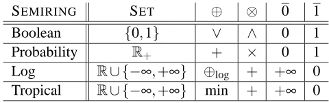
SEMIRING SET ⊕ ⊗ 0 1 Boolean {0,1} ∨ ∧ 0 1 Probability R+ + × 0 1 Log R∪ {−∞,+∞} ⊕log + +∞ 0 Tropical R∪ {−∞,+∞} min + +∞ 0
Table 1: Semiring examples. ⊕log is defined by x⊕logy=−log(e−x+e−y).
show that rational kernels are easy to design and implement and lead to substantial improvements of the classification accuracy.
The paper is organized as follows. In the following section, we introduce the notation and some preliminary algebraic and automata-theoretic definitions used in the remaining sections. Section 3 introduces the definition of rational kernels. In Section 4, we present general algorithms that can be used to compute rational kernels efficiently. Section 5 introduces the classical definitions of positive definite and negative definite kernels and gives a number of novel theoretical results, including the proof of some general closure properties of PDS rational kernels, a general construction of PDS rational kernels starting from an arbitrary weighted transducer, a characterization of acyclic PDS rational kernels, and the proof of the closure properties of a very general class of PDS rational ker-nels. Section 6 studies the relationship between some commonly used kernels and rational kerker-nels. Finally, the results of our experiments in several spoken-dialog classification tasks are reported in Section 7.
2. Preliminaries
In this section, we present the algebraic definitions and notation needed to introduce rational kernels. A system(K,,e)is a monoid if it is closed under: ab∈Kfor all a,b∈K;is associative:
(ab)c=a(bc) for all a,b,c∈K; and e is an identity for: ae=ea=a, for all
a∈K. When additionallyis commutative: ab=ba for all a,b∈K, then(K,,e)is said to be a commutative monoid.
Definition 1 (Kuich and Salomaa (1986)) A system (K,⊕,⊗,0,1) is a semiring if: (K,⊕,0) is
a commutative monoid with identity element 0; (K,⊗,1) is a monoid with identity element 1; ⊗
distributes over⊕; and 0 is an annihilator for⊗: for all a∈K,a⊗0=0⊗a=0.
Thus, a semiring is a ring that may lack negation. Table 1 lists some familiar semirings. In addition to the Boolean semiring and the probability semiring, two semirings often used in applications are the log semiring which is isomorphic to the probability semiring via a log morphism, and the
tropical semiring which is derived from the log semiring using the Viterbi approximation.
Definition 2 A weighted finite-state transducer T over a semiringKis an 8-tuple T= (Σ,∆,Q,I,F,E,λ,ρ)
whereΣis the finite input alphabet of the transducer;∆is the finite output alphabet; Q is a finite set of states; I⊆Q the set of initial states; F⊆Q the set of final states; E⊆Q×(Σ∪ {ε})×(∆∪ {ε})×K×Q a finite set of transitions;λ: I→Kthe initial weight function; andρ: F→Kthe
Weighted automata can be formally defined in a similar way by simply omitting the input or output
labels.
Given a transition e∈E, we denote by p[e]its origin or previous state and n[e]its destination state or next state, and w[e]its weight. A pathπ=e1· · ·ek is an element of E∗ with consecutive transitions: n[ei−1] = p[ei], i=2, . . . ,k. We extend n and p to paths by setting n[π] =n[ek]and
p[π] = p[e1]. A cycleπis a path whose origin and destination coincide: p[π] =n[π]. A weighted automaton or transducer is said to be acyclic if it admits no cycle. A successful path in a weighted automaton or transducer M is a path from an initial state to a final state. The weight function w can also be extended to paths by defining the weight of a path as the⊗-product of the weights of its constituent transitions: w[π] =w[e1]⊗ · · · ⊗w[ek]. We denote by P(q,q0)the set of paths from q to
q0 and by P(q,x,y,q0)the set of paths from q to q0 with input label x∈Σ∗and output label y∈∆∗. These definitions can be extended to subsets R,R0⊆Q, by P(R,x,y,R0) =∪q∈R,q0∈R0P(q,x,y,q0). We denote by w[M]the⊕-sum of the weights of all the successful paths of the automaton or transducer
M, when that sum is well-defined and in K. A transducer T is regulated if the output weight associated by T to any pair of input-output string(x,y)by
[[T]](x,y) = M π∈P(I,x,y,F)
λ(p[π])⊗w[π]⊗ρ[n[π]]
is well-defined and inK.[[T]](x,y) =0 when P(I,x,y,F) =/0. If for all q∈Q, the sumL
π∈P(q,ε,ε,q)w[π]
is inK, then T is regulated. In particular, when T does not have anyε-cycle, that is a cycle labeled withε(both input and output labels), it is regulated. In the following, we will assume that all the transducers considered are regulated. Regulated weighted transducers are closed under the rational operations:⊕-sum,⊗-product and Kleene-closure which are defined as follows for all transducers
T1and T2and(x,y)∈Σ∗×∆∗:
[[T1⊕T2]](x,y) = [[T1]](x,y)⊕[[T2]](x,y),
[[T1⊗T2]](x,y) =
M
x=x1x2,y=y1y2
[[T1]](x1,y1)⊗[[T2]](x2,y2),
[[T∗]](x,y) = ∞ M
n=0
Tn(x,y),
where Tnstands for the(n−1)-⊗-product of T with itself.
For any transducer T , we denote by T−1its inverse, that is the transducer obtained from T by transposing the input and output labels of each transition and the input and output alphabets.
Composition is a fundamental operation on weighted transducers that can be used in many
appli-cations to create complex weighted transducers from simpler ones. Let T1= (Σ,∆,Q1,I1,F1,E1,λ1,ρ1) and T2= (∆,Ω,Q2,I2,F2,E2,λ2,ρ2)be two weighted transducers defined over a commutative semir-ingKsuch that∆, the output alphabet of T1, coincides with the input alphabet of T2. Then, the result of the composition of T1 and T2is a weighted transducer T1◦T2which, when it is regulated, is de-fined for all x,y by (Berstel, 1979; Eilenberg, 1974; Salomaa and Soittola, 1978; Kuich and Salomaa,
1986)2
[[T1◦T2]](x,y) =
M
z∈∆∗
[[T1]](x,z)⊗[[T2]](z,y).
Note that a transducer can be viewed as a matrix over a countable setΣ∗×∆∗and composition as the corresponding matrix-multiplication.
The definition of composition extends naturally to weighted automata since a weighted automa-ton can be viewed as a weighted transducer with identical input and output labels for each transi-tion. The corresponding transducer associates[[A]](x)to a pair(x,x), and 0 to all other pairs. Thus, the composition of a weighted automaton A1= (∆,Q1,I1,F1,E1,λ1,ρ1)and a weighted transducer
T2= (∆,Ω,Q2,I2,F2,E2,λ2,ρ2)is simply defined for all x,y in∆∗×Ω∗by
[[A1◦T2]](x,y) =
M
x∈∆∗
[[A1]](x)⊗[[T2]](x,y)
when these sums are well-defined and inK. Intersection of two weighted automata is the special case of composition where both operands are weighted automata, or equivalently weighted trans-ducers with identical input and output labels for each transition.
3. Definitions
Let X and Y be non-empty sets. A function K : X×Y →R is said to be a kernel over X×Y . This section introduces rational kernels, which are kernels defined over sets of strings or weighted automata.
Definition 3 A kernel K over Σ∗×∆∗ is said to be rational if there exist a weighted transducer
T= (Σ,∆,Q,I,F,E,λ,ρ)over the semiringKand a functionψ:K→Rsuch that for all x∈Σ∗and
y∈∆∗:3
K(x,y) =ψ([[T]](x,y)).
K is then said to be defined by the pair(ψ,T).
This definition and many of the results presented in this paper can be generalized by replacing the free monoidsΣ∗and∆∗with arbitrary monoids M1 and M2. Also, note that we are not making any particular assumption about the functionψin this definition. In general, it is an arbitrary function mappingKtoR.
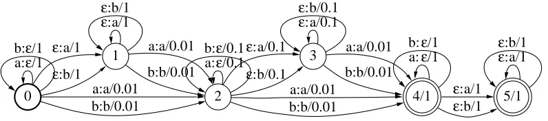
Figure 1 shows an example of a weighted transducer over the probability semiring correspond-ing to the gappy n-gram kernel with decay factorλas defined by (Lodhi et al., 2001). Such gappy
n-gram kernels are rational kernels (Cortes et al., 2003c).
Rational kernels can be naturally extended to kernels over weighted automata. Let A be a weighted automaton defined over the semiringKand the alphabetΣand B a weighted automaton defined over the semiringKand the alphabet∆, K(A,B)is defined by
K(A,B) =ψ
M
(x,y)∈Σ∗×∆∗
[[A]](x)⊗[[T]](x,y)⊗[[B]](y)
(1)
0 a:ε/1 b:ε/1
1 ε:a/1 ε:b/1
2 a:a/0.01
b:b/0.01 ε:a/1 ε:b/1
a:a/0.01
b:b/0.01 a:ε/0.1 b:ε/0.1
3 ε:a/0.1 ε:b/0.1
4/1 a:a/0.01
b:b/0.01 ε:a/0.1 ε:b/0.1
a:a/0.01
b:b/0.01 a:ε/1 b:ε/1
5/1 ε:a/1 ε:b/1
ε:a/1 ε:b/1
Figure 1: Gappy bigram rational kernel with decay factorλ=.1. Bold face circles represent initial states and double circles indicate final states. Inside each circle, the first number indicates the state number, the second, at final states only, the value of the final weight functionρ at that state. Arrows represent transitions. They are labeled with an input and an output symbol separated by a colon and followed by their corresponding weight after the slash symbol.
for all weighted automata A and B such that the⊕-sum
M
(x,y)∈Σ∗×∆∗
[[A]](x)⊗[[T]](x,y)⊗[[B]](y)
is well-defined and inK. This sum is always defined and inKwhen A and B are acyclic weighted automata since the sum then runs over a finite set. It is defined for all weighted automata in all closed
semirings (Kuich and Salomaa, 1986) such as the tropical semiring. In the probability semiring, the
sum is well-defined for all A, B, and T representing probability distributions. When K(A,B) is defined, Equation 1 can be equivalently written as
K(A,B) =ψ
M
(x,y)∈Σ∗×∆∗
[[A◦T◦B]](x,y)
=ψ(w[A◦T◦B]). (2)
The next section presents a general algorithm for computing rational kernels.
4. Algorithms
The algorithm for computing K(x,y), or K(A,B), for any two acyclic weighted automata, or for any two weighted automata such that the sum above is well-defined, is based on two general algorithms that we briefly present: composition of weighted transducers to combine A, T , and B, and a general shortest-distance algorithm in a semiringKto compute the⊕-sum of the weights of all successful paths of the composed transducer.
4.1 Composition of weighted transducers
0
1 a:a/1.61
2 b:b/0.22
a:b/0b:a/0.69
3/0
b:a/0.69 0
a:a/1.2
1 a:b/2.3 b:a/0.51
b:b/0.92
2/0 a:a/0.51
(a) (b)
0
1 a:a/2.81
4 a:b/3.91
2
b:a/0.73
a:a/0.51
a:b/0.92
3/0 b:a/1.2
(c)
Figure 2: (a) Weighted transducer T1over the log semiring. (b) Weighted transducer T2over the log semiring. (c) T1◦T2, result of the composition of T1and T2.
a state of T1and a state of T2. Leaving aside transitions withεinputs or outputs, the following rule specifies how to compute a transition of T1◦T2from appropriate transitions of T1and T2:4
(q1,a,b,w1,q2) and (q01,b,c,w2,q02) =⇒((q1,q01),a,c,w1⊗w2,(q2,q02)).
In the worst case, all transitions of T1leaving a state q1match all those of T2leaving state q01, thus the space and time complexity of composition is quadratic: O((|Q1|+|E1|)(|Q2|+|E2|)). Figure 2 illustrates the algorithm when applied to the transducers of Figure 2 (a)-(b) defined over the log semiring.
4.2 Single-source shortest distance algorithm over a semiring
Given a weighted automaton or transducer M, the shortest-distance from state q to the set of final states F is defined as the⊕-sum of all the paths from q to F,
d[q] = M π∈P(q,F)
w[π]⊗ρ[n[π]], (3)
when this sum is well-defined and in K. This is always the case when the semiring is k-closed or when M is acyclic (Mohri, 2002), the case of interest in our experiments. There exists a gen-eral algorithm for computing the shortest-distance d[q](Mohri, 2002). The algorithm is based on a generalization to k-closed semirings of the relaxation technique used in classical single-source shortest-paths algorithms. When M is acyclic, the complexity of the algorithm is linear: O(|Q|+ (T⊕+T⊗)|E|), where T⊕ denotes the maximum time to compute⊕ and T⊗ the time to compute ⊗ (Mohri, 2002). The algorithm can then be viewed as a generalization of Lawler’s algorithm (Lawler, 1976) to the case of an arbitrary semiringK. It is then based on a generalized relaxation of the outgoing transitions of each state of M visited in reverse topological order (Mohri, 2002).
Let K be a rational kernel and let T be the associated weighted transducer. Let A and B be two acyclic weighted automata or, more generally, two weighted automata such that the sum in Equation 2 is well-defined and inK. A and B may represent just two strings x,y∈Σ∗or may be any complex weighted automata. By definition of rational kernels (Equation 2) and the shortest-distance (Equation 3), K(A,B)can be computed by:
1. Constructing the composed transducer N=A◦T◦B.
2. Computing w[N], by determining the shortest-distance from the initial states of N to its final states using the shortest-distance algorithm just described.
3. Computingψ(w[N]).
When A and B are acyclic, the shortest-distance algorithm is linear and the total complexity of the algorithm is O(|T||A||B|+Φ), where|T|,|A|, and|B|denote respectively the size of T , A and B andΦthe worst case complexity of computingψ(x), x∈K. If we assume thatΦcan be computed in constant time as in many applications, then the complexity of the computation of K(A,B) is quadratic with respect to A and B: O(|T||A||B|).
5. Theory of PDS and NDS Rational Kernels
In learning techniques such as those based on SVMs, we are particularly interested in kernels that are positive definite symmetric (PDS), or, equivalently, kernels verifying Mercer’s condition, which guarantee the existence of a Hilbert space and a dot product associated to the kernel considered. This ensures the convergence of the training algorithm to a unique optimum. Thus, in what follows, we will focus on theoretical results related to the construction of rational kernels that are PDS. Due to the symmetry condition, the input and output alphabetsΣand∆will coincide for the underlying transducers associated to the kernels.
This section reviews a number of results related to general PDS kernels, that is the class of all kernels that have the Mercer property (Berg et al., 1984). It also gives novel proofs and results in the specific case of PDS rational kernels. These results can be used to combine PDS rational kernels to design new PDS rational kernels or to construct a PDS rational kernel. Our proofs and results are original and are not just straightforward extensions of those existing in the case of general PDS kernels. This is because, for example, a closure property for PDS rational kernels must guarantee not just that the PDS property is preserved but also that the rational property is retained. Our original results include a general construction of PDS rational kernels from arbitrary weighted transducers, a number of theorems related to the converse, and a study of the negative definiteness of some rational kernels.
Definition 4 Let X be a non-empty set. A function K : X×X→Ris said to be a PDS kernel if it is
symmetric(K(x,y) =K(y,x)for all x,y∈X)and
n
∑
i,j=1
cicjK(xi,xj)≥0
It is clear from classical results of linear algebra that K is a PDS kernel iff the matrix K(xi,xj)i,j≤n for all n≥1 and all{x1, . . . ,xn} ⊆X is symmetric and all its eigenvalues are non-negative.
PDS kernels can be used to construct other families of kernels that also meet these conditions (Sch¨olkopf and Smola, 2002). Polynomial kernels of degree p are formed from the expression
(K+a)p, and Gaussian kernels can be formed as exp(−d2/σ2)with d2(x,y) =K(x,x) +K(y,y)− 2K(x,y). The following sections will provide other ways of constructing PDS rational kernels.
5.1 General Closure Properties of PDS Kernels
The following theorem summarizes general closure properties of PDS kernels (Berg et al., 1984).
Theorem 5 Let X and Y be two non-empty sets.
1. Closure under sum: Let K1,K2: X×X →Rbe PDS kernels, then K1+K2: X×X →Ris a
PDS kernel.
2. Closure under product: Let K1,K2: X×X →Rbe PDS kernels, then K1·K2: X×X →Ris
a PDS kernel.
3. Closure under tensor product: Let K1: X×X→Rand K2: Y×Y →Rbe PDS kernels, then
their tensor product K1K2:(X×Y)×(X×Y)→R, where K1K2((x1,y1),(x2,y2)) =
K1(x1,x2)·K2(y1,y2)is a PDS kernel.
4. Closure under pointwise limit: Let Kn: X×X→Rbe a PDS kernel for all n∈Nand assume
that limn→∞Kn(x,y)exists for all x,y∈X , then K defined by K(x,y) =limn→∞Kn(x,y) is a
PDS kernel.
5. Closure under composition with a power series: Let K : X×X →Rbe a PDS kernel such
that|K(x,y)|<ρfor all(x,y)∈X×X . Then if the radius of convergence of the power series S=∑∞n=0anxnisρand an≥0 for all n≥0, the composed kernel S◦K is a PDS kernel. In
particular, if K : X×X→Ris a PDS kernel, then so is exp(K).
In particular, these closure properties all apply to PDS kernels that are rational, e.g., the sum or product of two PDS rational kernels is a PDS kernel. However, Theorem 5 does not guarantee the result to be a rational kernel. In the next section, we examine precisely the question of the closure properties of PDS rational kernels (under rational operations).
5.2 Closure Properties of PDS Rational Kernels
In this section, we assume that a fixed functionψis used in the definition of all the rational kernels mentioned. We denote by KT the rational kernel corresponding to the transducer T and defined for all x,y∈Σ∗by K
T(x,y) =ψ([[T]](x,y)).
1. Closure under ⊕-sum: Assume thatψ:(K,⊕,0)→(R,+,0) is a monoid morphism.5 Let KT1,KT2:Σ
∗×Σ∗→Rbe PDS rational kernels, then K
T1⊕T2 :Σ
∗×Σ∗→Ris a PDS rational
kernel and KT1⊕T2=KT1+KT2.
2. Closure under⊗-product: Assume thatψ:(K,⊕,⊗,0,1)→(R,+,×,0,1)is a semiring
mor-phism. Let KT1,KT2 :Σ
∗×Σ∗→Rbe PDS rational kernels, then K
T1⊗T2 :Σ
∗×Σ∗→Ris a
PDS rational kernel.
3. Closure under Kleene-closure: Assume thatψ:(K,⊕,⊗,0,1)→(R,+,×,0,1)is a
continu-ous semiring morphism. Let KT:Σ∗×Σ∗→Rbe a PDS rational kernel, then KT∗:Σ∗×Σ∗→ Ris a PDS rational kernel.
Proof The closure under⊕-sum follows directly from Theorem 5 and the fact that for all x,y∈Σ∗:
ψ([[T1]](x,y)⊕[[T2]](x,y)) =ψ([[T1]](x,y)) +ψ([[T2]](x,y))
whenψ:(K,⊕,0)→(R,+,0)is a monoid morphism. For the closure under⊗-product, whenψis a semiring morphism, for all x,y∈Σ∗:
ψ([[T1⊗T2]](x,y)) =
∑
x1x2=x,y1y2=yψ([[T1]](x1,y1))·ψ([[T2]](x2,y2))
=
∑
x1x2=x,y1y2=y
KT1KT2((x1,x2),(y1,y2)).
By Theorem 5, since KT1 and KT2 are PDS kernels, their tensor product KT1KT2 is a PDS kernel
and there exists a Hilbert space H⊆RΣ∗ and a mapping u→φusuch that KT
1KT2(u,v) =hφu,φvi
(Berg et al., 1984). Thus
ψ([[T1⊗T2]](x,y)) =
∑
x1x2=x,y1y2=yhφ(x1,x2),φ(y1,y2)i
=
*
∑
x1x2=x
φ(x1,x2),
∑
y1y2=y
φ(y1,y2)
+
.
Since a dot product is positive definite, this equality implies that KT1⊗T2 is a PDS kernel. A similar
proof is given by Haussler (1999). The closure under Kleene-closure is a direct consequence of the closure under⊕-sum and⊗-product of PDS rational kernels and the closure under pointwise limit of PDS kernels (Theorem 5).
Theorem 6 provides a general method for constructing complex PDS rational kernels from simpler ones. PDS rational kernels defined to model specific prior knowledge sources can be combined using rational operations to create a more general PDS kernel.
In contrast to Theorem 6, PDS rational kernels are not closed under composition. This is clear since the ordinary matrix multiplication does not preserve positive definiteness in general.
The next section studies a general construction of PDS rational kernels using composition.
5.3 A General Construction of PDS Rational Kernels
In this section, we assume thatψ:(K,⊕,⊗,0,1)→(R,+,×,0,1)is a continuous semiring mor-phism. This limits the choice of the semiring associated to the weighted transducer defining a rational kernel, since it needs in particular to be commutative and non-idempotent.6 Our study of PDS rational kernels in this section is thereby limited to such semirings. This should not leave the reader with the incorrect perception that all PDS rational kernels are defined over non-idempotent semirings though. As already mentioned before, in general, the functionψcan be chosen arbitrarily and needs not impose any algebraic property on the semiring used.
We show that there exists a general way of constructing a PDS rational kernel from any weighted transducer T . The construction is based on composing T with its inverse T−1.
Proposition 7 Let T = (Σ,∆,Q,I,F,E,λ,ρ)be a weighted finite-state transducer defined over the semiring (K,⊕,⊗,0,1). Assume that the weighted transducer T◦T−1 is regulated, then (ψ,T◦
T−1)defines a PDS rational kernel overΣ∗×Σ∗.
Proof Denote by S the composed transducer T◦T−1. Let K be the rational kernel defined by S. By definition of composition,
K(x,y) =ψ([[S]](x,y)) =ψ M
z∈∆∗
[[T]](x,z)⊗[[T]](y,z)
!
,
for all x,y∈Σ∗. Sinceψis a continuous semiring morphism, for all x,y∈Σ∗,
K(x,y) =ψ([[S]](x,y)) =
∑
z∈∆∗
ψ([[T]](x,z))·ψ([[T]](y,z)).
For all n∈Nand x,y∈Σ∗, define Kn(x,y)by
Kn(x,y) =
∑
|z|≤nψ([[T]](x,z))·ψ([[T]](y,z)),
where the sum runs over all strings z∈∆∗of length less than or equal to n. Clearly, K
ndefines a sym-metric kernel. For any l≥1 and any x1, . . . ,xl∈Σ∗, define the matrix Mnby Mn= (Kn(xi,xj))i≤l,j≤l. Let z1,z2, . . . ,zmbe an arbitrary ordering of the strings of length less than or equal to n. Define the matrix A by
A= (ψ([[T]](xi,zj)))i≤l; j≤m.
By definition of Kn, Mn=AAt. The eigenvalues of AAt are non-negative for any rectangular matrix
A, thus Kn is a PDS kernel. Since K is a pointwise limit of Kn, K(x,y) =limn→∞Kn(x,y), by Theorem 5, K is a PDS kernel. This ends the proof of the proposition.
The next propositions provide results related to the converse of Proposition 7. We denote by IdRthe
identity function overR.
Proposition 8 Let S= (Σ,Σ,Q,I,F,E,λ,ρ) be an acyclic weighted finite-state transducer over (K,⊕,⊗,0,1)such that(ψ,S)defines a PDS rational kernel onΣ∗×Σ∗, then there exists a weighted
transducer T over the probability semiring such that(IdR,T◦T−1)defines the same rational kernel.
Proof Let S be an acyclic weighted transducer verifying the hypotheses of the proposition. Let
X ⊂Σ∗ be the finite set of strings accepted by S. Since S is symmetric, X×X is the set of pairs
of strings (x,y) defining the rational relation associated with S. Let x1,x2, . . . ,xn be an arbitrary numbering of the elements of X . Define the matrix M by
M= (ψ([[S]](xi,xj)))1≤i≤n,1≤j≤n.
Since S defines a PDS rational kernel, M is a symmetric matrix with non-negative eigenvalues, i.e.,
M is symmetric positive definite. The Cholesky decomposition extends to the case of
semi-definite matrices (Dongarra et al., 1979): there exists an upper triangular matrix R= (Ri j) with non-negative diagonal elements such that M=RRt. Let Y ={y1, . . . ,yn}be an arbitrary subset of n distinct strings ofΣ∗. Define the weighted transducer T over the X×Y by
[[T]](xi,yj) =Ri j
for all i,j, 1≤i,j≤n. By definition of composition,[[T◦T−1]](xi,xj) =ψ([[S]](xi,xj))for all i,j, 1≤i,j≤n. Thus, T◦T−1=ψ(S), which proves the claim of the proposition.
Note that when the matrix M introduced in the proof is positive definite, that is when the eigenvalues of the matrix associated with S are all positive, then Cholesky’s decomposition and thus the weights associated to the input strings of T are unique.
Assume that the same continuous semiring morphismψis used in the definition of all the ratio-nal kernels.
Proposition 9 LetΘbe the subset of the weighted transducers over(K,⊕,⊗,0,1)such that for any
S∈Θ,(ψ,S)defines a PDS rational kernel and there exists a weighted transducer T= (Σ,∆,Q,I,F,E,λ,ρ) over the probability semiring such that(IdR,T◦T−1) defines the same rational kernel as (ψ,S).
ThenΘis closed under⊕-sum,⊗-product, and Kleene-closure.
Proof Let S1,S2∈Θ, we will show that S1⊕S2∈Θ, S1⊗S2∈Θ, and S∗1∈Θ. By definition, there exist T1= (Σ,∆1,Q1,I1,F1,E1,λ1,ρ1)and T2= (Σ,∆2,Q2,I2,F2,E2,λ2,ρ2)such that
K1=T1◦T1−1 and K2=T2◦T2−1,
where K1(K2) is the PDS rational kernel defined by(ψ,S1)(resp. (ψ,S2)). Let u be an alphabetic morphism mapping∆2to a new alphabet∆02such that∆1∩∆02=/0. u is clearly a rational transduction (Berstel, 1979) and can be represented by a finite-state transducer U . Thus, we can define a new weighted transducer T20 by T20=T2◦U = (Σ,∆02,Q2,I2,F2,E20,λ2,ρ2), which only differs from T2 by some renaming of its output labels. This does not affect the result of the composition with the inverse transducer since U◦U−1is the identity mapping over∆∗2:
T20◦T0−21=T2◦U◦(U−1◦T2−1) =T2◦T2−1=K2. (4) Since, T1and T2have distinct output alphabets, their output labels cannot match; thus
T1◦T0−21=/0 and T20◦T1−1= /0. (5)
Let T =T1+T20, in view of Equation 4 and Equation 5:
T◦T−1= (T1+T20)◦(T1+T20)−1= (T1◦T1−1) + (T02◦T0− 1
Since the same continuous semiring morphismψis used for the definition of all the rational kernels inΘ, by Theorem 6, K1+K2is a PDS rational kernel defined by(ψ,S1⊕S2)and S1⊕S2 is inΘ. Similarly, define T0as T0=T1·T20:
T0◦T0−1= (T1·T20)◦(T1·T20)−1= (T1◦T1−1)·(T2◦T0−21).
Thus, S1⊗S2 is inΘ. Let x be a symbol not in∆1 and let∆01=∆1∪ {x}. Let V be the finite-state transducer accepting as input onlyεand mappingεto x and define T10 by T10=V·T1. Since x does not match any of the output labels of T1, T10◦T10
−1=T
1◦T1−1and(T10◦T10
−1)∗=T0 1
∗◦(T0 1
−1)∗:
(T1◦T1−1)∗= (T10◦T10 −1
)∗=T10∗◦(T10−1)∗.
Thus, by Theorem 6, S∗1is a PDS rational kernel that is inΘ.
Proposition 9 raises the following question: under the same assumptions, are all PDS rational ker-nels defined by a pair of the form(ψ,T◦T−1)? A natural conjecture is that this is the case and that this property provides a characterization of the weighted transducers defining PDS rational kernels. Propositions 8 and 9 both favor that conjecture. Proposition 8 shows that this holds in the acyclic case. Proposition 9 might be useful to extend this to the general case.
In the case of PDS rational kernels defined by (IdR,S)with S a weighted transducer over the probability semiring, the conjecture could be reformulated as: is S of the form S=T◦T−1? If true, this could be viewed as a generalization of Cholesky’s decomposition theorem to the case of infinite matrices given by weighted transducers over the probability semiring.
This ends our discussion of PDS rational kernels. In the next section, we will examine negative
definite kernels and their relationship with PDS rational kernels.
5.4 Negative Definite Kernels
As mentioned before, given a set X and a distance or dissimilarity measure d : X×X →R+, a common method used to define a kernel K is the following. For all x,y∈X ,
K(x,y) =exp(−td2(x,y)),
where t>0 is some constant typically used for normalization. Gaussian kernels are defined in this way. However, such kernels K are not necessarily positive definite, e.g., for X=R, d(x,y) =|x−y|p,
p>1 and t =1, K is not positive definite. The positive definiteness of K depends on t and the properties of the function d. The classical results presented in this section exactly address such questions (Berg et al., 1984). They include a characterization of PDS kernels based on negative
definite kernels which may be viewed as distances with some specific properties.7
The results we are presenting are general, but we are particularly interested in the case where d can be represented by a rational kernel. We will use these results later when dealing with the case of the edit-distance.
Definition 10 Let X be a non-empty set. A function K : X×X→Ris said to be a negative definite symmetric kernel (NDS kernel) if it is symmetric(K(x,y) =K(y,x)for all x,y∈X)and
n
∑
i,j=1
cicjK(xi,xj)≤0
for all n≥1,{x1, . . . ,xn} ⊆X and{c1, . . . ,cn} ⊆Rwith∑ni=1ci=0.
Clearly, if K is a PDS kernel then−K is a NDS kernel, however the converse does not hold in
general. Negative definite kernels often correspond to distances, e.g., K(x,y) = (x−y)α, x,y∈R, with 0<α≤2 is a negative definite kernel.
The next theorem summarizes general closure properties of NDS kernels (Berg et al., 1984).
Theorem 11 Let X be a non-empty set.
1. Closure under sum: Let K1,K2: X×X→Rbe NDS kernels, then K1+K2: X×X→Ris a
NDS kernel.
2. Closure under log and exponentiation: Let K : X×X→Rbe a NDS kernel with K≥0, and
αa real number with 0<α<1, then log(1+K),Kα: X×X→Rare NDS kernels.
3. Closure under pointwise limit: Let Kn: X×X →Rbe a NDS kernel for all n∈N, then K
defined by K(x,y) =limn→∞Kn(x,y)is a NDS kernel.
The following theorem clarifies the relation between NDS and PDS kernels and provides in partic-ular a way of constructing PDS kernels from NDS ones (Berg et al., 1984).
Theorem 12 Let X be a non-empty set, xo∈X , and let K : X×X→Rbe a symmetric kernel.
1. K is negative definite iff exp(−tK)is positive definite for all t>0.
2. Let K0be the function defined by
K0(x,y) =K(x,x0) +K(y,x0)−K(x,y)−K(x0,x0).
Then K is negative definite iff K0is positive definite.
The theorem gives two ways of constructing a positive definite kernel using a negative definite kernel. The first construction is similar to the way Gaussian kernels are defined. The second con-struction has been put forward by (Sch ¨olkopf, 2001).
6. Relationship with some commonly used kernels or similarity measures
0/0 a:a/0 b:b/0 a:b/1 b:a/1ε:a/1
ε:b/1 a:ε/1 b:ε/1
0 a:a/1 a:b/1 b:a/1 b:b/1ε:a/1
ε:b/1 a:ε/1 b:ε/1
1/1 b:ε/1
b:a/1
ε:a/1
ε:b/1 a:ε/1 a:b/1
a:a/1 a:b/1 b:a/1 b:b/1ε:a/1
ε:b/1 a:ε/1 b:ε/1
(a) (b)
Figure 3: (a) Weighted transducer over the tropical semiring representing the edit-distance over the alphabet Σ={a,b}. (b) Weighted transducer over the probability semiring computing the cost of alignments over the alphabetΣ={a,b}.
6.1 Edit-Distance
A common similarity measure in many applications is that of the edit-distance, that is the minimal cost of a series of edit operations (symbol insertions, deletions, or substitutions) transforming one string into the other (Levenshtein, 1966). We denote by de(x,y) the edit-distance between two strings x and y over the alphabetΣwith cost 1 assigned to all edit operations.
Proposition 13 LetΣbe a non-empty finite alphabet and let de be the edit-distance overΣ, then
de is a symmetric rational kernel. Furthermore, (1): de is not a PDS kernel, and (2): de is a NDS
kernel iff|Σ|=1.
Proof The edit-distance between two strings, or weighted automata, can be represented by a simple weighted transducer over the tropical semiring (Mohri, 2003). Since the edit-distance is symmetric,
deis a symmetric rational kernel. Figure 3(a) shows the corresponding transducer when the alphabet isΣ={a,b}. The cost of the alignment between two sequences can also be computed by a weighted transducer over the probability semiring (Mohri, 2003), see Figure 3(b).
Let a∈Σ, then the matrix(de(xi,xj))1≤i,j≤2 with x1=ε and x2=a has a negative eigenvalue (−1), thus deis not a PDS kernel.
When|Σ|=1, the edit-distance simply measures the absolute value of the difference of length between two strings. A string x∈Σ∗can then be viewed as a vector of the Hilbert spaceR∞. Denote byk · kthe corresponding norm. For all x,y∈Σ∗,
*
* *
* * * *
*
all strings of length n
smallest eigenvalue
2 4 6 8
0.0 0.2 0.4 0.6
i 1 2 3 4 5
xi abc bad dab adc bcd
ci 1 1 −23 −23 −23
(a) (b)
Figure 4: (a) Smallest eigenvalue of the matrix Mn= (exp(−de(xi,xj)))1≤i,j,≤2n as a function of n.
(b) Example demonstrating that the edit-distance is not negative definite.
The square distancek · k2is negative definite, thus by Theorem 11, de= (k · k2)1/2is also negative definite.
Assume now that|Σ|>1. We show that exp(−de)is not PDS. By Theorem 12, this implies that
deis not negative definite. Let x1,· · ·,x2nbe any ordering of the strings of length n over the alphabet
{a,b}. Define the matrix Mnby
Mn= (exp(−de(xi,xj)))1≤i,j,≤2n.
Figure 4(a) shows the smallest eigenvalue αn of Mn as a function of n. Clearly, there are values of n for whichαn<0, thus the edit-distance is not negative definite. Table 4(b) provides a simple example with five strings of length 3 over the alphabetΣ={a,b,c,d}showing directly that the edit-distance is not negative definite. Indeed, it is easy to verify that∑5i=1∑5j=1cicjK(xi,xj) =23>0.
To our knowledge, this is the first statement and proof of the fact that de is not NDS for|Σ|>
1. This result has a direct consequence on the design of kernels in computational biology, often based on the edit-distance or other related similarity measures. The edit-distance and other related similarity measures are often used in computational biology. When|Σ|>1, Proposition 13 shows that de is not NDS. Thus, there exists t>0 for which exp(−tde) is not PDS. Similarly, de2 is not NDS since otherwise by Theorem 11, de= (de2)1/2would be NDS.
6.2 Haussler’s Convolution Kernels for Strings
D. Haussler describes a class of kernels for strings built by applying iteratively convolution kernels (Haussler, 1999). We show that these convolution kernels for strings are specific instances of ra-tional kernels. Haussler (1999) defines the convolution of two string kernels K1 and K2 over the alphabetΣas the kernel denoted by K1?K2and defined for all x,y∈Σ∗by
K1?K2(x,y) =
∑
x1x2=x,y1y2=yK1(x1,y1)·K2(x2,y2).
(1999) also introduces for 0≤γ<1 theγ-infinite iteration of a mapping H :Σ∗×Σ∗→Rby
Hγ∗= (1−γ) ∞
∑
n=1
γn−1H(n),
where H(n)=H?H(n−1) is the result of the convolution of H with itself n−1 times. Note that
Hγ∗=0 forγ=0.
Lemma 14 For 0<γ<1, theγ-infinite iteration of a rational transduction H :Σ∗×Σ∗→Rcan
be defined in the following way with respect to the Kleene †-operator:
Hγ∗=1−γ γ (γH)†.
Proof Haussler’s convolution simply corresponds to the product (or concatenation) in the case of rational transductions. Thus, for 0<γ<1, by definition of the †-operator,
(γH)†= ∞
∑
n=1
(γH)n= ∞
∑
n=1
γnHn= γ 1−γ
∞
∑
n=1
(1−γ)γn−1Hn= γ
1−γH ∗
γ .
Given a probability distribution p over all symbols ofΣ, Haussler’s convolution kernels for strings are defined by
KH(x,y) =γK2?(K1?K2)?γ+ (1−γ)K2,
where K1is the specific polynomial PDS rational transduction over the probability semiring defined by K1(x,y) =∑a∈Σp(x|a)p(y|a)p(a)and models substitutions, and K2another specific PDS rational transduction over the probability semiring modeling insertions.
Proposition 15 For any 0≤γ<1, Haussler’s convolution kernels KHcoincide with the following special cases of rational kernels:
KH= (1−γ)[K2(γK1K2)∗].
Proof As mentioned above, Haussler’s convolution simply corresponds to concatenation in this context. When γ=0, by definition, KH is reduced to K2 which is a rational transducer and the proposition’s formula above is satisfied. Assume now that γ6=0. By lemma 14, KH can be re-written as
KH = γK2(K1K2)?γ+ (1−γ)K2=γK2 1−γ
γ (γK1K2)†+ (1−γ)K2
= (1−γ)[K2(γK1K2)†+K2] = (1−γ)[K2(γK1K2)∗].
Since rational transductions are closed under rational operations, KH also defines a rational trans-duction. Since K1and K2are PDS kernels, by Theorem 6, KHdefines a PDS kernel.
0 (1 − γ)K2 1 γK1 2 K2
Figure 5: Haussler’s convolution kernels KH for strings: specific instances of rational kernels. K1, (K2), corresponds to a specific weighted transducer over the probability semiring and modeling substitutions (resp. insertions).
6.3 Other Kernels Used in Computational Biology
In this section we show the relationship between rational kernels and another class of kernels used in computational biology.
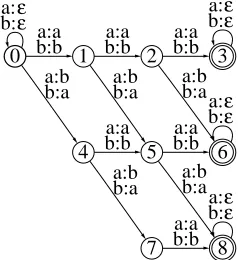
A family of kernels, mismatch string kernels, was introduced by (Leslie et al., 2003) for protein classification using SVMs. Let Σ be a finite alphabet, typically that of amino acids for protein sequences. For any two sequences z1,z2∈Σ∗ of same length (|z1|=|z2|), we denote by d(z1,z2) the total number of mismatching symbols between these sequences. For all m∈N, we define the bounded distance dmbetween two sequences of same length by
dm(z1,z2) =
1 if(d(z1,z2)≤m) 0 otherwise.
and for all k∈N, we denote by Fk(x)the set of all factors of x of length k:
Fk(x) ={z : x∈Σ∗zΣ∗,|z|=k}.
For any k,m∈Nwith m≤k, a(k,m)-mismatch kernel K(k,m):Σ∗×Σ∗→Ris the kernel defined over protein sequences x,y∈Σ∗by
K(k,m)(x,y) =
∑
z1∈Fk(x),z2∈Fk(y),z∈Σk
dm(z1,z)dm(z,z2).
Proposition 16 For any k,m∈Nwith m≤k, the(k,m)-mismatch kernel K(k,m):Σ∗×Σ∗→Ris a
PDS rational kernel.
Proof Let M, S, and D be the weighted transducers over the probability semiring defined by
M=
∑
a∈Σ
(a,a) S=
∑
a6=b
(a,b) D=
∑
a∈Σ
(a,ε).
M associates weight 1 to each pair of identical symbols of the alphabetΣ, S associates 1 to each pair of distinct or mismatching symbols, and D associates 1 to all pairs with second elementε.
For i,k∈Nwith 0≤i≤k, Define the shuffle of Siand Mk−i, denoted by SittMk−i, as the the sum over all products made of factors S and M with exactly i factors S and k−i factors M. As a finite
0 a:ε b:ε 1 a:a b:b 4 a:b b:a 2 a:a b:b 5 a:b b:a a:a b:b 7 a:b b:a 3 a:a b:b 6 a:b b:a a:a b:b 8 a:b b:a a:ε b:ε a:ε b:ε a:a b:b a:ε b:ε
Figure 6: Mismatch kernel K(k,m)=Tk,m◦Tk−1,m(Leslie et al., 2003) with k=3 and m=2 and with Σ={a,b}. The transducer T3,2 defined over the probability semiring is shown. All transition weights and final weights are equal to one. Note that states 3, 6, and 8 of the transducer are equivalent and thus can be merged and similarly that states 2 and 5 can then be merged as well.
any k,m∈Nwith m≤k: Tk,m=D∗RD∗ with R=∑mi
=0SittMk−i. Consider two sequences z1,z2 such that|z1|=|z2|=k. By definition of M and S and the shuffle product, for any i, with 0≤i≤m,
[[SittMk−i]](z1,z2) =
1 if(d(z1,z2) =i) 0 otherwise.
Thus, [[R]](z1,z2) = m
∑
i=0
SittMk−i(z1,z2) =
1 if(d(z1,z2)≤m) 0 otherwise
= dm(z1,z2).
By definition of the product of weighted transducers, for any x∈Σ∗and z∈Σk,
Tk,m(x,z) =
∑
x=uvw,z=u0v0w0[[D∗]](u,u0) [[R]](v,v0) [[D∗]](w,w0)
=
∑
v∈Fk(x),z=v0
[[R]](v,v0) =
∑
v∈Fk(x)
dm(v,z).
It is clear from the definition of Tk,m that Tk,m(x,z) =0 for all x,z∈Σ∗ with |z|>k. Thus, by definition of the composition of weighted transducer, for all x,y∈Σ∗
[[Tk,m◦Tk,m−1]](x,y) =
∑
z1∈Fk(x),z2∈Fk(y),z∈Σ∗
dm(z1,z)dm(z,z2)
=
∑
z1∈Fk(x),z2∈Fk(y),z∈Σk
dm(z1,z)dm(z,z2) =K(k,m)(x,y).
Figure 6 shows T3,2, a simple weighted transducer over the probability semiring that can be
used to compute the mismatch kernel K(3,2)=T3,2◦T3,2−1. Such transducers provide a compact representation of the kernel and are very efficient to use with the composition algorithm already described in (Cortes et al., 2003c). The transitions of these transducers can be defined implicitly and expanded on-demand as needed for the particular input strings or weighted automata. This substantially reduces the space needed for their representation, e.g., a single transition with labels
x : y, x6=y can be used to represent all transitions with similar labels ((a : b), a,b∈Σ, with a6=b).
Similarly, composition can also be performed on-the-fly. Furthermore, the transducer of Figure 6 can be made more compact since it admits several states that are equivalent.
7. Applications and Experiments
Rational kernels can be used in a variety of applications ranging from computational biology to optical character recognition. We have applied them successfully to a number of speech process-ing tasks includprocess-ing the identification from speech of traits, or voice signatures, such as emotion (Shafran et al., 2003). This section describes some of our most recent applications to spoken-dialog classification.
We first introduce a general family of PDS rational kernels relevant to spoken-dialog classifi-cation tasks that we used in our experiments, then discuss the spoken-dialog classificlassifi-cation problem and report our experimental results.
7.1 A General Family of PDS Kernels: n-gram Kernels
A rational kernel can be viewed as a similarity measure between two sequences or weighted au-tomata. One may for example consider two utterances to be similar when they share many common
n-gram subsequences. The exact transcriptions of the utterances are not available but we can use
the word lattices output by the recognizer instead.
A word lattice is a weighted automaton over the log semiring that compactly represents the most likely transcriptions of a speech utterance. Each path of the automaton is labeled with a sequence of words whose weight is obtained by adding the weights of the constituent transitions. The weight assigned by the lattice to a sequence of words can often be interpreted as the log-likelihood of that transcription based on the models used by the recognizer. More generally, the weights are used to rank possible transcriptions, the sequence with the lowest weight being the most favored transcription.
A word lattice A can be viewed as a probability distribution PA over all strings s∈Σ∗. Modulo a normalization constant, the weight assigned by A to a string x is[[A]](x) =−log PA(x). Denote by|s|xthe number of occurrences of a sequence x in the string s. The expected count or number of occurrences of an n-gram sequence x in s for the probability distribution PAis
c(A,x) =
∑
s
PA(s)|s|x.
Two lattices output by a speech recognizer can be viewed as similar when the sum of the product of the expected counts they assign to their common n-gram sequences is sufficiently high. Thus, we define an n-gram kernel knfor two lattices A1and A2by
kn(A1,A2) =
∑
|x|=n0 a:ε/1 b:ε/1
1 a:a/1
b:b/1 2/1
a:a/1 b:b/1
a:ε/1 b:ε/1
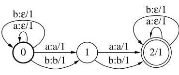
Figure 7: Weighted transducer T computing expected counts of bigram sequences of a word lattice withΣ={a,b}.
The kernel knis a PDS rational kernel of type T◦T−1and it can be computed efficiently.
Indeed, there exists a simple weighted transducer T that can be used to computed c(A1,x)for all
n-gram sequences x∈Σ∗. Figure 7 shows that transducer in the case of bigram sequences (n=2) and for the alphabetΣ={a,b}. The general definition of T is
T = (Σ× {ε})∗(
∑
x∈Σ
{x} × {x})n(Σ× {ε})∗.
kncan be written in terms of the weighted transducer T as
kn(A1,A2) = w[(A1◦T)◦(T−1◦A2)]
= w[(A1◦(T◦T−1)◦A2)],
which shows that it is a rational kernel whose associated weighted transducer is T◦T−1. In view of Proposition 7, knis a PDS rational kernel. Furthermore, the general composition algorithm and shortest-distance algorithm described in Section 4 can be used to compute kn efficiently. The size of the transducer T is O(n|Σ|) but in practice, a lazy implementation can be used to simulate the presence of the transitions of T labeled with all elements ofΣ. This reduces the size of the machine used to O(n). Thus, since the complexity of composition is quadratic (Mohri et al., 1996; Pereira and Riley, 1997) and since the general shortest distance algorithm just mentioned is linear for acyclic graphs such as the lattices output by speech recognizers (Mohri, 2002), the worst case complexity of the algorithm is O(n2|A1| |A2|).
By Theorem 6, the sum of two kernels kn and kmis also a PDS rational kernel. We define an
n-gram rational kernel Kn as the PDS rational kernel obtained by taking the sum of all km, with 1≤m≤n:
Kn= n
∑
m=1
km.
Thus, the feature space associated with Kn is the set of all m-gram sequences with m≤n. n-gram
kernels are used in our experiments in spoken-dialog classification.
7.2 Spoken-Dialog Classification 7.2.1 DEFINITION
Dataset Number of Training Testing Number of ASR word classes size size n-grams accuracy HMIHY 0300 64 35551 5000 24177 72.5%
VoiceTone1 97 29561 5537 22007 70.5% VoiceTone2 82 9093 5172 8689 68.8%
Table 2: Key characteristics of the three datasets used in the experiments. The fifth column displays the total number of unigrams, bigrams, and trigrams found in the one-best output of the ASR for the utterances of the training set, that is the number of features used by BoosTexter or SVMs used with the one-best outputs.
a speech recognizer. The choice of possible categories depends on the dialog context considered. A category may correspond to the type of billing problem in the context of a dialog related to billing, or to the type of problem raised by the speaker in the context of a hot-line service. Categories are used to direct the dialog manager in formulating a response to the speaker’s utterance. Classification is typically based on features such as relevant key words or key sequences used by a machine learning algorithm.
The word error rate of conversational speech recognition systems is still too high in many tasks to rely only on the one-best output of the recognizer (the word error rate in the deployed services we have experimented with is about 70%, as we will see later). However, the word lattices output by speech recognition systems may contain the correct transcription in most cases. Thus, it is preferable to use instead the full word lattices for classification.
The application of classification algorithms to word lattices raises several issues. Even small word lattices may contain billions of paths, thus the algorithms cannot be generalized by simply applying them to each path of the lattice. Additionally, the paths are weighted and these weights must be used to guide appropriately the classification task. The use of rational kernels solves both of these problems since they define kernels between weighted automata and since they can be com-puted efficiently (Section 4).
7.2.2 DESCRIPTION OFTASKS ANDDATASETS
We did a series of experiments in several large-vocabulary spoken-dialog tasks using rational kernels with a twofold objective: to improve classification accuracy in those tasks, and to evaluate the impact on classification accuracy of the use a word lattice rather than the one-best output of the automatic speech recognition (ASR) system.
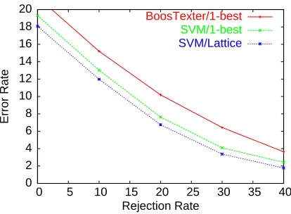
0 2 4 6 8 10 12 14 16 18 20
0 5 10 15 20 25 30 35 40
Error Rate
Rejection Rate BoosTexter/1-best
SVM/1-best SVM/Lattice
Figure 8: Classification error rate as a function of rejection rate in HMIHY 0300.
Table 7.2.2 indicates the size of the HMIHY 0300 datasets we used for training and testing. The training set is relatively large with more than 35,000 utterances, this is an extension of the one we used in our previous classification experiments with HMIHY 0300 (Cortes et al., 2003c). In our experiments, we used the n-gram rational kernels described in the previous section with n=3. Thus, the feature set we used was that of all n-grams with n≤3. Table 7.2.2 indicates the total number of distinct features of this type found in the datasets. The word accuracy of the system based on the best hypothesis of the speech recognizer is 72.5%. This motivated our use of the word lattices, which may contain the correct transcription in most cases. The average number of transitions of a word lattice in this task was about 260.
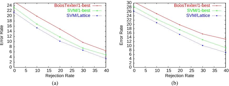
Table 7.2.2 reports similar information for two other datasets, VoiceTone1, and VoiceTone2. These are more recently deployed spoken-dialog systems in different areas, e.g., VoiceTone1 is a task where users interact with a system related to health-care with a larger set of categories (97). The size of the VoiceTone1 datasets we used and the word accuracy of the recognizer (70.5%) make this task otherwise similar to HMIHY 0300. The datasets provided for VoiceTone2 are significantly smaller with a higher word error rate. The word error rate is indicative of the difficulty of classifi-cation task since a higher error rate implies a more noisy input. The average number of transitions of a word lattice in VoiceTone1 was about 210 and in VoiceTone2 about 360.
Each utterance of the dataset may be labeled with several classes. The evaluation is based on the following criterion: it is considered an error if the highest scoring class given by the classifier is none of these labels.
7.2.3 IMPLEMENTATION ANDRESULTS