High Dimensional Inverse Covariance Matrix Estimation
via Linear Programming
Ming Yuan [email protected]
School of Industrial and Systems Engineering Georgia Institute of Technology
Atlanta, GA 30332-0205, USA
Editor: John Lafferty
Abstract
This paper considers the problem of estimating a high dimensional inverse covariance matrix that can be well approximated by “sparse” matrices. Taking advantage of the connection between mul-tivariate linear regression and entries of the inverse covariance matrix, we propose an estimating procedure that can effectively exploit such “sparsity”. The proposed method can be computed using linear programming and therefore has the potential to be used in very high dimensional prob-lems. Oracle inequalities are established for the estimation error in terms of several operator norms, showing that the method is adaptive to different types of sparsity of the problem.
Keywords: covariance selection, Dantzig selector, Gaussian graphical model, inverse covariance matrix, Lasso, linear programming, oracle inequality, sparsity
1. Introduction
One of the classical problems in multivariate statistics is to estimate the covariance matrix or its inverse. Let X = (X1, . . . ,Xp)′ be a p-dimensional random vector with an unknown covariance
matrixΣ0. The goal is to estimateΣ0or its inverseΩ0:=Σ−01based on n independent copies of X , X(1), . . . ,X(n). The usual sample covariance matrix is most often adopted for this purpose:
S=1 n
n
∑
i=1
(X(i)−X¯)(X(i)−X¯)′,
and Yu (2008), Rocha, Zhao and Yu (2008), Lam and Fan (2009), and Rothman, Levina and Zhu (2009) among others.
Bickel and Levina (2008a) pioneered the theoretical study of high dimensional sparse covariance matrices. They consider the case where the magnitude of the entries ofΣ0 decays at a polynomial rate of their distance from the diagonal; and show that banding the sample covariance matrix or S leads to well-behaved estimates. More recently, Cai, Zhang and Zhou (2010) established min-imax convergence rates for estimating this type of covariance matrices. A more general class of covariance matrix model is investigated in Bickel and Levina (2008b) where the rows or columns ofΣ0 is assumed to come from an ℓαball with 0<α<1. They suggest thresholding the entries of S and study its theoretical behavior when p is large. In addition to the aforementioned methods, sparse models have also been proposed for the modified Cholesky factor of the covariance matrix in a series of papers by Pourahmadi and co-authors (Pourahmadi, 1999; Pourahmadi, 2000; Wu and Pourahmadi, 2003; Huang et al., 2006).
In this paper, we focus on another type of sparsity—sparsity in terms of the entries of the inverse covariance matrix. This type of sparsity naturally connects with the problem of covariance selection (Dempster, 1972) and Gaussian graphical models (see, e.g., Whittaker, 1990; Lauritzen, 1996; Ed-wards, 2000), which makes it particularly appealing in a number of applications. Methods to exploit such sparsity have been proposed recently. Inspired by the nonnegative garrote (Breiman, 1995) and Lasso (Tibshirani, 1996) for the linear regression, Yuan and Lin (2007) propose to imposeℓ1type of penalty on the entries of the inverse covariance matrix when maximizing the normal log-likelihood and therefore encourages some of the entries of the estimated inverse covariance matrix to be exact zero. Similar approaches are also taken by Banerjee, El Ghaoui and d’Aspremont (2008). One of the main challenges for this type of methods is computation which has been recently addressed by d’Aspremont, Banerjee and El Ghaoui (2008), Friedman, Hastie and Tibshirani (2008), Rocha, Zhao and Yu (2008), Rothman et al. (2008) and Yuan (2008). Some theoretical properties of this type of methods have also been developed by Yuan and Lin (2007), Ravikumar et al. (2008), Roth-man et al. (2008) and Lam and Fan (2009) among others. In particular, the results from Ravikumar et al. (2008) and Rothman et al. (2008) suggest that, although better than the sample covariance matrix, these methods may not perform well when p is larger than the sample size n. It remains unclear to what extent the sparsity of inverse covariance matrix entails well-behaved covariance matrix estimates.
Through the study of a new estimating procedure, we show here that the estimability of a high dimensional inverse covariance matrix is related to how well it can be approximated by a graphical model with a relatively low degree. The revelation that the degree of a graph dictates the diffi-culty of estimating a high dimensional covariance matrix suggests that the proposed method may be more appropriate to harness sparsity in the inverse covariance matrix than those mentioned earlier in which theℓ1penalty serves as a proxy to control the total number of edges in the graph as opposed to its degree. The proposed method proceeds in two steps. A preliminary estimate is first con-structed using a well known relationship between inverse covariance matrix and multivariate linear regression. We show that the preliminary estimate, although often dismissed as an estimate of the inverse covariance matrix, can be easily modified to produce a satisfactory estimate for the inverse covariance matrix. We show that the resulting estimate enjoys very good theoretical properties by establishing oracle inequalities for the estimation error.
in-equalities are demonstrated on a couple of popular covariance matrix models. WhenΩ0corresponds to a Gaussian graphical model of degree d, we show that the proposed method can achieve conver-gence rate of the order Op[d(n−1log p)−1/2]in terms of several matrix operator norms. We also
examine the more general case where the rows or columns ofΩ0belong to anℓαball (0<α<1), the family of positive definite matrices introduced by Bickel and Levina (2008b). We show that the proposed method achieves the convergence rate of Op[(n−1log p)(1−α)/2], the same as that obtained
by Bickel and Levina (2008b) when assuming thatΣ0rather thanΩ0belongs to the same family of matrices. For both examples, we also show that the obtained rates are optimal in a minimax sense when considering estimation error in terms of matrixℓ1orℓ∞norms.
The proposed method shares similar spirits with the neighborhood selection approach proposed by Meinshausen and B¨uhlmann (2006). However, the two techniques are developed for different purposes. Neighborhood selection aims at identifying the correct graphical model whereas our goal is to estimate the covariance matrix. The distinction is clear when the inverse covariance matrix is only “approximately” sparse and does not have many zero entries. Even when the inverse covariance matrix is indeed sparse, the two tasks of estimation and selection can be different. In particular, our results suggest that good estimation can be achieved under conditions weaker than those often assumed to ensure good selection.
The rest of the paper is organized as follows. In the next section, we describe in details the estimating procedure. Theoretical properties of the method are established in Section 3. All detailed proofs are relegated to Section 6. Numerical experiments are presented in Section 4 to illustrate the merits of the proposed method before concluding with some remarks in Section 5.
2. Methodology
In what follows, we shall write X−i= (X1, . . . ,Xi−1,Xi+1, . . . ,Xp)′. Similarly, denote byΣ−i,−j the
submatrix ofΣwith its ith row and jth column removed. Other notation can also be interpreted in the same fashion. For example,Σi,−jorΣ−i,jrepresents the ith row ofΣwith its j entry removed or
the jth column with its ith entry removed respectively.
2.1 Regression and Inverse Covariance Matrix
It is well known that if X follows a multivariate normal distribution
N
(µ,Σ), then the conditional distribution of Xigiven X−i remains normally distributed (Anderson, 2003), that is,Xi|X−i∼
N
µi+Σi,−iΣ−−1i,−i(X−i−µ−i),Σii−Σi,−iΣ−−1i,−iΣ−i,i
.
This can be equivalently expressed as the following regression equation:
Xi=αi+X−′iθ(i)+εi, (1)
whereαi=µi−Σi,−iΣ−−1i,−iµ−iis a scalar,θ(i)=Σ−−1i,−iΣ−i,iis a p−1 dimensional vector andεi∼
N
(0,Σii−Σi,−iΣ−−i,1−iΣ−i,i) is independent of X−i. When X follows a more general distribution,similar relationship holds in that αi+X−′iθ(i) is the best linear unbiased estimate of Xi given X−i
Now by the inverse formula for block matrices,Ω:=Σ−1is given by
Σ
11 Σ1,−1
Σ−1,1 Σ−1,−1
−1
=
Ω11
z }| {
Σ11−Σ1,−1Σ−−11,−1Σ−1,1
−1
−Ω11Σ1,−1Σ−−11,−1 −Σ−1
−1,−1Σ−1,1Ω11 ∗
.
More generally, the ith column ofΩcan be written as
Ωii = Σii−Σi,−iΣ−−1i,−iΣ−i,i
−1
;
Ω−i,i = −
Σii−Σi,−iΣ−−1i,−iΣ−i,i
−1
Σ−1
−i,−iΣ−i,i.
This immediately connects with (1):
Ωii = (Var(εi))−1;
Ω−i,i = −(Var(εi))−1θ(i).
Therefore, an estimate ofΩcan potentially be obtained by regressing Xi over X−i for i=1, . . . ,p.
Furthermore, the sparsity in the entries ofΩcan be translated into sparsity in regression coefficients
θ(i)s.
2.2 Initial Estimate
From the aforementioned relationship, a zero entry on the ith column of the inverse covariance matrix implies a zero entry in the regression coefficientθ(i)and vice versa. This property is exploited by Meinshausen and B¨uhlmann (2006) to identify the zero pattern of the inverse covariance matrix. Specifically, in the so-called neighborhood selection method, the zero entries of the ith column of
Ω0are identified by doing variable selection when regressing Xi over X−i. More specifically, they
suggest to use Lasso (Tibshirani, 1996) for the purpose of variable selection.
Our goal here, however, is rather different. Instead of identifying which entries ofΩ0are zero, our focus is on estimating it. The distinction is apparent whenΩ0is only “approximately” sparse instead of having a lot of zero entries. Even ifΩ0indeed has lot of zeros, the two tasks can still be quite different in high dimensional problems. For example, in identifying the nonzero entries of
Ω0, it is necessary to assume that all nonzero entries are sufficiently different from zero (see, e.g., Meinshausen and B¨uhlmann, 2006). Such assumptions may be unrealistic and can be relaxed if the purpose is to estimate the covariance matrix. With such a distinction in mind, the question now is whether or not similar strategies of applying sparse multivariate linear regression to recover the inverse covariance matrix remains useful. The answer is affirmative.
To this end, we consider estimatingΩ0as follows: ˜
Ωii = Var(c εi)−1; ˜
Ω−i,i = −
c
Var(εi)−1θˆ(i),
whereVar(c εi) and ˆθ(i)are estimated from regressing Xi over X−i. In particular, we suggest to use
begin by centering each variable Xito eliminate the interceptαiin (1). Denote by Zi=Xi−X¯iwhere
¯
Xiis the sample average of Xi. The Dantzig selector estimate ofθ(i)is the solution to
min β∈Rp−1,β
0∈R
kβkℓ1 subject to
En Zi−Z−′iβ
Z−iℓ∞≤δ,
whereEnrepresents the sample average, andδ>0 is a tuning parameter. Recall thatEnZiZj=Si j.
The above problem can also be written in terms of S:
min β∈Rp−1,β
0∈R
kβkℓ1 subject to
S−i,i−S−i,−iβ
ℓ∞ ≤δ. (2)
The minimization of theℓ1norm of the regression coefficient reflects our preference towards sparse models which is particularly important when dealing with high dimensional problems. Once an estimate ofθ(i)is obtained, we can then estimate the variance ofεiby the mean squared error of the residuals:
c
Var(εi) =En Xi−X−′iθˆ(i)
2
=Sii−2 ˆθ′(i)S−i,i+θˆ′(i)S−i,−iθˆ(i).
We obtain ˜Ωby repeating this procedure for i=1, . . . ,p.
We emphasize that for practical purposes, one can also use the Lasso in place of the Dantzig selector for constructing ˜Ω. The choice of Dantzig selector is made for the sake of our further technical developments. In the light of the results of Bickel, Ritov and Tsybakov (2009), similar performance can be expected with either the Lasso or the Dantzig selector although a more rigorous proof when using the Lasso is beyond the scope of the current paper.
2.3 Symmetrization
˜
Ωis is usually dismissed as an estimate ofΩfor it is not even symmetric. In fact, it is not obvi-ous that ˜Ωis in any sense a reasonable estimate ofΩ0. But a more careful examination suggests otherwise. It reveals that ˜Ωcould be a good estimate in a certain matrix operator norm.
The matrix operator norm is a class of matrix norms induced by vector norms. Letkxkℓq be the
ℓqnorm of an p dimensional vector x= (x1, . . . ,xp)′, that is,
kxkℓq= (|x1|
q+. . .+|x p|q)1/q.
Then the matrixℓqnorm for an p×p square matrix A= (ai j)1≤i,j≤pis given by
kAkℓq=sup
x6=0 kAxkℓq
kxkℓq
.
In the case of q=1 and q=∞, the matrix norm can be given more explicitly as
kAkℓ1 = max
1≤j≤p p
∑
i=1
ai j
;
kAkℓ∞ = max
1≤i≤p p
∑
j=1
ai j
.
A careful study shows that ˜Ωcan be a good estimate ofΩin terms of the matrixℓ1 norm in sparse circumstances. It is therefore of interest to consider improved estimates from ˜Ωthat inherits this property. To this end, we propose to adjust ˜Ωby seeking a symmetric matrix ˆΩthat is the the closest to ˜Ωin the sense of the matrixℓ1norm, that is, it solves the following problem:
min
Ωis symmetrickΩ− ˜
Ωkℓ1. (3)
Recall that
kΩ−Ω˜kℓ1 = max
1≤j≤p p
∑
i=1
Ωi j−Ωi j˜ .
Problem (3) can therefore be re-formulated as a linear program just like the computation of ˜Ω. To sum up, our estimate of the inverse covariance matrix is obtained in the following steps:
ALGORITHM FORCOMPUTINGΩˆ
Input: Sample covariance matrix – S, tuning parameter –δ.
Output: An estimate of the inverse covariance matrix – ˆΩ.
• Construct ˜Ω for i=1 to p
– Estimateθ(i)by ˆθ(i), the solution to
min
β∈Rp−1kβkℓ1 subject to
S−i,i−S−i,−iβ
ℓ∞ ≤δ.
– Set
˜
Ωii=Sii−2 ˆθ(′i)S−i,i+θˆ′(i)S−i,−iθˆ(i)
−1
.
– Set
˜
Ω−i,i=−Ωii˜ θˆ(i).
end
• Construct ˆΩ
– Set ˆΩas the solution to
min
Ωis symmetrickΩ− ˜
Ωkℓ1.
3. Theory
In what follows, we shall assume that the components of X are uniformly sub-gaussian, that is, there exist constants c0≥0, and T >0 such that for any|t| ≤T
EetXi2 ≤c0, i=1,2, . . . ,p.
This condition is clearly satisfied when X follows a multivariate normal distribution. It also holds true when Xis are bounded.
3.1 Oracle Inequality
Our main tool to study the theoretical properties of ˆΩ is an oracle type of inequality regarding the estimation error kΩˆ −Ω0kℓ1. To this end, we introduce the following set of “oracle” inverse
covariance matrices:
O
(ν,η,τ) =
Ω≻0 :
ν−1≤λmin(Ω)≤λmax(Ω)≤ν (Bounded Eigenvalues)
kΣ0Ω−Ikmax≤η (“Good” Approximation)
kΩkℓ1 ≤τ (Sparsity)
,
where A≻0 indicates that a matrix A is symmetric and positive definite;ν>1,τ>0, andη≥0 are parameters; λmin andλmaxrepresent the smallest and largest eigenvalue respectively; andk · kmax represents the entry-wiseℓ∞norm, that is,
kAkmax= max 1≤i,j≤p|ai j|.
We refer to
O
(ν,η,τ)as an “oracle” set because its definition requires the knowledge of the true covariance matrixΣ0. Every member ofO
(ν,η,τ)is symmetric, positive definite with eigenvalues bounded away from 0 and∞, and belongs to anℓ1ball. Moreover,O
(ν,η,τ)consists of matrices that approximateΩ0well. It is worth noting that different from the usual vector case, the choice of metric is critical when evaluating approximating error for matrices. In particular for our purpose, the approximation error is measured bykΣ0Ω−Ikmax, which vanishes if and only ifΩ=Ω0. We are now in position to state our main result.Theorem 1 There exist constants C1,C2 depending only on ν,τ, λmin(Ω0) andλmax(Ω0), and C3 depending only on c0such that, for any A>0, with probability at least 1−p−A,
Ωˆ −Ω0
ℓ1≤C1Ω∈Oinf(ν,η,τ)
Ω−Ω0
ℓ1+deg(Ω)δ
, (4)
provided that
inf Ω∈O(ν,η,τ)
Ω−Ω0
ℓ1+deg(Ω)δ
≤C2, (5)
and
We remark that the oracle inequality given in Theorem 1 is of probabilistic nature and non-asymptotic. However, (4) holds with overwhelming probability as we are interested in the case when p is very large. The requirement (5) is in place to ensure that the true inverse covariance matrix is indeed “approximately” sparse. Another note is on the choice of the tuning parameter
δ. To ensure an tight upper bound in (4), smallerδs are preferred. On the other hand, Condition (6) specifies how small they can be. For simplicity, we have used the same tuning parameterδfor estimating allθ(i)s. In practice, it may be beneficial to use differentδs for differentθ(i)s. Following the same argument, it can be shown that the statement of Theorem 1 continue to hold if all tuning parameters used satisfy Condition (6).
Recall that for a symmetric matrix A,kAkℓ∞=kAkℓ1 and
kAkℓ2≤(kAkℓ1kAkℓ∞)
1/2
=kAkℓ1.
A direct consequence of Theorem 1 is that the same upper bound holds true under matrixℓ∞andℓ2 norms.
Corollary 2 There exist constants C1,C2 depending only onν,τ, λmin(Ω0)andλmax(Ω0), and C3 depending only on c0such that, for any A>0, with probability at least 1−p−A,
Ωˆ −Ω0
ℓ∞,
Ωˆ −Ω0
ℓ2 ≤C1Ω∈Oinf(ν,η,τ)
Ω−Ω0
ℓ1+deg(Ω)δ
,
provided that
inf Ω∈O(ν,η,τ)
Ω−Ω0
ℓ1+deg(Ω)δ
≤C2, and
δ≥νη+C3ντλ−min1(Ω0)((A+1)n−1log p)1/2.
The bound on the matrixℓ2has great practical implications when we are interested in estimating the covariance matrix or need to a positive definite estimate of Ω. The proposed estimate ˆΩ is symmetric but not guaranteed to be positive definite. However, Corollary 2 suggests that with overwhelming probability, it is indeed positive definite provided that the upper bound is sufficiently small because
λmin(Ωˆ)≥λmin(Ω0)−
Ωˆ −Ω0
ℓ2.
Moreover, a positive definite estimate of Ω can always be constructed by replacing its negative eigenvalues withδ. Denote the resulting estimate byΩˆˆ. By Corollary 2, it can be shown that
Corollary 3 There exist constants C1,C2 depending only onν,τ, λmin(Ω0)andλmax(Ω0), and C3 depending only on c0such that, for any A>0, with probability at least 1−p−A,
Ωˆˆ−1−Σ 0
ℓ2,
Ωˆˆ −Ω0
ℓ2≤C1Ω∈Oinf(ν,η,τ)
Ω−Ω0
ℓ1+deg(Ω)δ
,
provided that
inf Ω∈O(ν,η,τ)
Ω−Ω0
ℓ1+deg(Ω)δ
≤C2, and
When considering a particular class of inverse covariance matrices, we can use the oracle in-equalities established here with a proper choice of the oracle set
O
. Typically in choosing a good oracle setO
, we takeνandτto be of finite magnitude whereas the approximation errorηsufficiently small. To further illustrate their practical implications, we now turn to a couple of more concrete examples.3.2 Sparse Models
We begin with a class of matrix models that are closely connected with graphical models. When X follows a multivariate normal distribution, the sparsity of the entries of the inverse covariance matrix relates to the notion of conditional independence: the(i,j)entry ofΩ0being zero implies that Xi is independent of Xjconditional on the remaining variables and vice versa. The conditional
independence relationships among the coordinates of the Gaussian random vector X can be repre-sented by an undirected graph G= (V,E), often referred to as a Gaussian graphical model, where V contains p vertices corresponding to the p coordinates and the edge between Xi and Xjis present if
and only if Xiand Xj are not independent conditional on the others. The complexity of a graphical
model is commonly measured by its degree:
deg(G) = max 1≤i≤p
∑
j ei j,where ei j =1 if there is an edge between Xi and Xj and 0 otherwise. Gaussian graphical models
are an indispensable statistical tool in studying communication networks and gene pathways among many other subjects. The readers are referred to Whittaker (1990), Lauritzen (1996) and Edwards (2000) for further details.
Motivated by this connection, we consider the following class of inverse covariance matrices:
M
1(τ0,ν0,d) =
A≻0 :kAkℓ1<τ0,ν
−1
0 <λmin(A)<λmax(A)<ν0,deg(A)<d ,
where τ0,ν0>1, and deg(A) =maxi∑jI(Ai j 6=0). In this case, taking an oracle set such that Ω0∈
O
yields the following result:Theorem 4 Assume that d(n−1log p)1/2=o(1). Then sup
Ω0∈M1(τ0,ν0,d)
Ωˆ −Ω0
ℓq =Op d
r
log p n
!
, (7)
provided thatδ=C(n−1log p)1/2and C is large enough.
Theorem 4 follows immediately from Theorem 1 and Corollary 2 by takingη=0,τ=kΩ0kℓ1,
andν=max{λ−min1(Ω0),λmax(Ω0)}, which ensures thatΩ0∈
O
(ν,η,τ). We note that the rate of convergence given by (7) is also optimal in the minimax sense when considering matrixℓ1norm.Theorem 5 Assume that d(n−1log p)1/2=o(1). Then there exists a constant C>0 depending only onτ0, andν0such that
inf ¯
Ω Ω0∈Msup1(τ0,ν0,d)
P
(
Ω¯ −Ω0
ℓ1 ≥Cd
r
log p n
)
>0,
Theorem 5 indicates that the estimability of a sparse inverse covariance matrix is dictated by its degree as opposed to the total number of nonzero entries. This observation gives a plausible expla-nation on why the usualℓ1penalized likelihood estimate (see, e.g., Yuan and Lin, 2007; Banarjee, El Ghaoui and d’Aspremont, 2008) may not be the best to exploit this type of sparsity because the penalty employed by these methods is convex relaxations of the constraint on total number of edges in a graphical model instead of its degree.
It is also of interest to compare our results with those from Meinshausen and B¨uhlmann (2006). As mentioned before, the goal of the neighborhood selection from Meinshausen and B¨uhlmann (2006) is to select the correct graphical model whereas our focus here is on estimating the covariance matrix. However, the neighborhood selection method can be followed by the maximum likelihood estimation based on the selected graphical model to yield a covariance matrix estimate. Clearly the success of this method hinges upon the ability of the neighborhood selection to choose a correct graphical model. It turns out that selecting the graphical model can be more difficult than estimating the covariance matrix as reflected by the more restrictive assumptions made in Meinshausen and B¨uhlmann (2006). In particular, to be able to identify the nonzero entries of the inverse covariance matrix, it is necessary that they are sufficiently large in magnitude whereas such requirement is generally not needed for the purpose of estimation. Moreover, Meinshausen and B¨uhlmann (2006) only deals with the case when the dimensionality is of a polynomial order of the sample size, that is, p=O(nγ)for someγ>0.
3.3 Approximately Sparse Models
In many applications, the inverse covariance matrix is only approximately sparse. A popular way to model this class of covariance matrix is to assume that its rows or columns belong to anℓαball (0<α<1):
M
2(τ0,ν0,α,M) =
A≻0 :kA−1kℓ1 <τ0,ν
−1
0 ≤λmin(A)≤λmax(A)≤ν0,
p
∑
j=1
Ai j
α≤M
,
where τ0,ν0>1 and 0<α<1.
M
2 can be viewed as a natural extension of the sparse modelM
1. In particular,M
1can be viewed as the limiting case ofM
2whenαapproaches 0. By relaxingα,
M
2 includes matrices that are less sparse than those included inM
1. The particular class of matrices were first introduced by Bickel and Levina (2008b) who investigate the case whenΣ0∈M
2(τ0,ν0,α,M). We note that their setting is different from ours asM
2is not closed with respect to inversion. An application of Theorem 1 and Corollary 2 yields:Theorem 6 Assume that M n−1log p
1−α
2 =o(1). Then
sup Ω0∈M2(τ0,ν0,α,M)
kΩˆ −Ω0kℓq=Op M
log p n
1−α
2 !
, (8)
provided thatδ=C(n−1log p)1/2and C is sufficiently large.
however interesting to note that Bickel and Levina (2008b) show that thresholding the sample co-variance matrix S at an appropriate level can achieve the same rate given by right hand side of (8). The coincidence should not come as a surprise despite the difference in problem setting because the size of the parameter space in both problems are the same. Moreover, the following theorem shows that in both settings, the rate is optimal in the minimax sense.
Theorem 7 Assume that M n−1log p
1−α
2 =o(1). Then there exists a constant C>0 depending
only onτ0, andν0such that
inf ¯
Ω Ω0∈M2sup(τ0,ν0,α,M)
P
(
Ω¯ −Ω0
ℓ1≥CM
log p n
1−α
2
)
>0, (9)
and
inf ¯
Σ Σ0∈M2sup(τ0,ν0,α,M)
P
(
Σ¯−Σ0
ℓ1≥CM
log p n
1−α
2
)
>0, (10)
where the infimum is taken over all estimate, ¯Ωor ¯Σ, based on observations X(1), . . . ,X(n).
4. Numerical Experiments
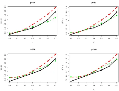
To illustrate the merits of the proposed method and compare it with other popular alternatives, we now conduct a set of numerical studies. Specifically, we generated n=50 observations from a multivariate normal distribution with mean 0 and variance covariance matrix given byΣ0i j =ρ|i−j|
for someρ6=0. Such covariance structure corresponds to an AR(1) model. Its inverse covariance matrix is banded with the magnitude of ρdetermining the strength of the dependence among the coordinates. We consider combinations of seven different values ofρ, 0.1, 0.2,. . . , 0.7 and four val-ues of the dimensionality, p=25, 50, 100 or 200. Two hundred data sets were simulated for each combination. For each simulated data set, we ran the proposed method to construct estimate of the inverse covariance matrix. As suggested by the theoretical developments, we setδ= (2n−1log p)−1 throughout all simulation studies. For comparison purposes, we included a couple of popular alter-native covariance matrix estimates in the study. The first is theℓ1penalized likelihood estimate of Yuan and Lin (2007). As suggested by Yuan and Lin (2007), the BIC criterion was used to choose the tuning parameter among a total of 20 pre-specified values. The second is a variant of the neigh-borhood selection approach of Meinshausen and B¨uhlmann (2006). As pointed out earlier, the goal of the neighborhood selection is to identify the underlying graphical model rather than estimating the covariance matrix. We consider here a simple two-step procedure where the maximum likeli-hood estimate based on the selected graphical model is employed. As advocated by Meinshausen and B¨uhlmann (2006), the level of significance is set atα=0.05 in identifying the graphical model. Figure 1 summarizes the estimation error measured by the spectral norm, that is,kCˆ−Ckℓ2, for the
three methods, averaged over two hundred runs.
0.1 0.2 0.3 0.4 0.5 0.6 0.7
0.8
1.0
1.2
1.4
1.6
1.8
2.0
p=25
ρ
||C
^−C||
0.1 0.2 0.3 0.4 0.5 0.6 0.7
0.8
1.0
1.2
1.4
1.6
1.8
2.0
p=50
ρ
||C
^−C||
0.1 0.2 0.3 0.4 0.5 0.6 0.7
0.8
1.0
1.2
1.4
1.6
1.8
2.0
p=100
ρ
||C
^−C||
0.1 0.2 0.3 0.4 0.5 0.6 0.7
0.8
1.0
1.2
1.4
1.6
1.8
2.0
p=200
ρ
||C
^−C||
Figure 1: Estimation error of the proposed method (black solid lines), theℓ1penalized likelihood estimate (red dashed lines) and the maximum likelihood estimate based on the graphical model selected through neighborhood selection (green dotted lines). Each panel corre-sponds to a different value of the dimensionality. X-axes represent the value ofρ. The estimation errors are averaged over two hundred runs.
of the graphical model. Recall that the inverse covariance matrix is banded with nonzero entries increasing in magnitude withρ. For large values ofρ, the task of identifying the correct graphical model is relatively easier. With a good graphical model chosen, refitting it with the maximum likelihood estimator could reduce biases often associated with regularization approaches. Such benefit diminishes for small values of ρas identifying nonzero entries in the inverse covariance matrix becomes more difficult.
and available in theglassopackage in R. The proposed method is implemented inMATLABusing its general purpose interior-point algorithm based linear programming solver and could be further improved using more specialized algorithms (see, e.g., Asif, 2008).
5. Discussions
High dimensional (inverse) covariance matrix estimation is becoming more and more common in various scientific and technological areas. Most of the existing methods are designed to benefit from sparsity of the covariance matrix, and based on banding or thresholding the sample covari-ance matrix. Sparse models for the inverse covaricovari-ance matrix, despite its practical appeal and close connection to graphical modeling, are more difficult to be taken advantage of due to heavy computa-tional cost as well as the lack of a coherent theory on how such sparsity can be effectively exploited. In this paper, we propose an estimating procedure that addresses both challenges. The proposed method can be formulated using linear programming and therefore computed very efficiently. We also show that the resulting estimate enjoys nice probabilistic properties, which translates to sharp convergence rates in terms of matrix operator norms under a couple of common settings.
The choice of the tuning parameter δis of great practical importance. Our theoretical devel-opments have suggested reasonable choices of the tuning parameter and it seems to work well in the well-controlled simulation settings. In practice, however, a data-driven choice such as those determined by multi-fold cross-validation may yield improved performance.
We also note that the method can be easily extended to handle prior information regarding the sparsity patterns of the inverse covariance matrices. Such situations often arise in the context of, for example, genomics. In a typical gene expression experiment, tens of thousands of genes are often studied simultaneously. Among these genes, there are often known pathways which corresponding to conditional (in)dependence among a subset of the genes, or in our notation, variables. This can be naturally interpreted as some of the entries ofΩ0being known to be nonzero or zero. Such prior information can be easily incorporated in our procedure. In particular, it suffices to set some of the entries ofβto be exact zero apriori in (2). Likewise, if a particular entry of βis known to be nonzero, we can also opt to minimize theℓ1norm of only the remaining entries.
6. Proofs
We now present the proofs to Theorems 1, 5, 6 and 7.
6.1 Proof of Theorem 1
We begin by comparing ˆθ(i) withθ(i). For brevity, we shall abbreviate the subscript (i) in what follows when no confusion occurs. Recall thatθ=−Ω0
−i,i/Ω0iiand
ˆ
θ=argmin β∈F
kβkℓ1,
where
F
={β:kS−i,i−S−i,−iβkℓ∞≤δ}. For a givenΩ∈O
(ν,η,τ), letΩ∈O
andγ=−Ω−i,i/Ωii.We first show thatγ∈
F
.provided that
δ≥ην+C0τνλmax(Σ0)((A+1)n−1log p)1/2.
Proof By the definition of
O
(ν,η,τ), for any j6=i,Σ0
j·Ω·i
=ΩiiΣ0ji−Σ0j,−iγ≤ kΣ0Ω−Ikmax≤η, which implies that
Σ0
−i,i−Σ0−i,−iγ
ℓ∞=maxj6=i Σ0
ji−Σ0j,−iγ
≤Ω−1
ii η≤λ−min1(Ω)η≤ην. An application of the triangular inequality now yields
kS−i,i−S−i,−iγkℓ∞ ≤
S−i,i−Σ0−i,i
ℓ∞+
S−i,−i−Σ0−i,−i
γ
ℓ∞+ Σ0
−i,i−Σ0−i,−iγ
ℓ∞
≤ kS−Σ0kmax+kS−Σ0kmaxkγkℓ1+ην
= kS−Σ0kmaxkΩ·ikℓ1/Ωii+ην
≤ τνkS−Σ0kmax+ην. The claim now follows.
Now thatγ∈
F
, by the definition of ˆθ,kθˆkℓ1 ≤ kγkℓ1 ≤Ω
−1
ii kΩ·ikℓ1−1≤λ
−1
min(Ω)kΩkℓ1−1≤ντ−1. (11)
Write
J
={j :γj6=0}. Denote by dJ =card(J
). It is clear that dJ ≤deg(Ω). From (11),0≤ kγkℓ1− kθˆkℓ1≤ kθˆJ −γJkℓ1− kθˆJckℓ1.
Thus,
kθˆ−γkℓ1 = kθˆJ −γJkℓ1+kθˆJckℓ1
≤ 2kθˆJ −γJkℓ
1
≤ 2dJ1/2kθˆJ−γJkℓ2
≤ 2dJ1/2kθˆ−γkℓ2
≤ 2dJ1/2λ−min1(Σ0−i,−i)h θˆ−γ′Σ0−i,−i θˆ−γi1/2 ≤ 2λ−min1(Σ0)dJ1/2
h
ˆ
θ−γ′Σ0−i,−i θˆ−γi1/2 = 2λmax(Ω0)dJ1/2
h
ˆ
θ−γ′Σ0
−i,−i θˆ−γ
i1/2
.
Observe that
ˆ
θ−γ′Σ0−i,−i θˆ−γ≤ kθˆ−γkℓ1
Σ0
−i,−i θˆ−γℓ∞.
Therefore,
kθˆ−γkℓ
1 ≤2λmax(Ω0)d
1/2
J kθˆ−γk
1/2
ℓ1
Σ0
−i,−i θˆ−γ
1/2
which implies that
kθˆ−γkℓ1≤4λ
2
max(Ω0)dJ
Σ0
−i,−i θˆ−γℓ∞. (12)
We now set up to further bound the last term on the right hand side. We appeal to the following result.
Lemma 9 Under the event thatkS−Σ0kmax<C0λmax(Σ0)((A+1)n−1log p)1/2, we have
Σ0
−i,−i θˆ−γℓ∞ ≤2δ,
provided that
δ≥ην+C0τνλmax(Σ0)((A+1)n−1log p)1/2.
Proof By triangular inequality,
Σ0
−i,−i θˆ−γℓ∞≤
Σ0
−i,−i(θ−γ)
ℓ∞+ Σ0
−i,−i θˆ−θℓ∞. (13)
We begin with the first term on the right hand side. Recall that
Σ0
−i,iΩ0ii+Σ0−i,−iΩ0−i,−i=0,
which implies that
Σ0
−i,−iθ=Σ0−i,i. (14)
Hence,
Σ0
−i,−i(θ−γ)
ℓ∞ = Σ0
−i,i−Σ0−i,−iγ
ℓ∞ =Ω −1
ii
Σ0
−i,iΩii+Σ0−i,−iΩ−i,i
ℓ∞≤νη.
We now turn to the second term on the right hand side of (13). Again by triangular inequality
Σ0
−i,−i θˆ−θℓ∞≤
S−i,−i−Σ0−i,−i
θˆ
ℓ∞+
S−i,−iθˆ−Σ0−i,−iθ
ℓ∞.
To bound the first term on the right hand side, note that
S−i,−i−Σ0−i,−i
θˆ
ℓ∞≤
S−i,−i−Σ0−i,−i
maxkθˆkℓ1≤ kS−Σ0kmaxkθˆkℓ1.
Also recall that
S−i,i−S−i,−iθˆ
ℓ∞ ≤δ,
andΣ0−i,−iθ=Σ0
−i,i. Therefore, by triangular inequality and (14),
S−i,−iθˆ−Σ0−i,−iθ
ℓ∞ ≤δ+kΣ
0
−i,i−S−i,ikℓ∞ ≤δ+kS−Σ0kmax. To sum up,
Σ0
−i,−i θˆ−γℓ∞ ≤ δ+νη+kS−Σ0kmax+kS−Σ0kmaxkθˆkℓ1
≤ δ+νη+kS−Σ0kmax(1+kγkℓ1)
≤ δ+νη+kS−Σ0kmaxkΩkℓ1/Ωii
≤ δ+νη+kS−Σ0kmaxkΩkℓ1λ
which, under the event thatkS−Σ0kmax<C0λmax(Σ0)((A+1)n−1log p)1/2, can be further bounded by 2δby Lemma 8.
Together with (12), Lemma 9 implies that for all i=1, . . . ,p
kθˆ−γkℓ1 ≤8λ
2
max(Ω0)dJδ,
ifkS−Σ0kmax<C0λmax(Σ0)((A+1)n−1log p)1/2. We are now in position to bound kΩ˜ −Ω0kℓ1.
We begin with the diagonal elements|Ωii˜ −Ω0
ii|.
Lemma 10 Assume thatkS−Σ0kmax<C0λmax(Σ0)((A+1)n−1log p)1/2and
δλmax(Ω0) ντ+8λ2max(Ω0)λ−min1(Ω0)dJ
+ντλmax(Ω0)λ−min2(Ω0)kΩ−Ω0kℓ1≤c0
for some numerical constant 0<c0<1. Then
Ω0
ii−Ωii˜
≤ 1
1−c0
δλ2
max(Ω0) ντ+8λ2max(Ω0)dJλ−min1(Ω0)
+ντλ−min2(Ω0)λ2max(Ω0)kΩ−Ω0kℓ1
,
provided that
δ≥ην+C0τνλmax(Σ0)((A+1)n−1log p)1/2.
Proof Recall thatΣ0−i,i=Σ0
−i,−iθ. Therefore
Ω0
ii= Σ0ii−2Σ0i,−iθ+θ′Σ0−i,−iθ
−1
= Σ0
ii−Σ0i,−iθ
−1
.
Because
˜
Ωii= Sii−2Si,−iθˆ+θˆ′S−i,−iθˆ
−1
,
we have
Ω˜−ii1− Ω0ii
−1
≤ |Sii−Σ0ii|+
θˆ′S
−i,−iθˆ−Si,−iθˆ
+Si,−iθˆ−Σ0i,−iθ
. (15)
We now bound the three terms on the right hand side separately. It is clear that the first term can be bounded bykS−Σ0kmax. Recall that ˆθ∈
F
. Hence the second term can be bounded as follows:θˆ′S
−i,−iθˆ−Si,−iθˆ
≤S−i,−iθˆ−S−i,i
ℓ∞kθˆkℓ1≤δkθˆkℓ1.
The last term on the right hand side of (15) can also be bounded similarly.
Si,−iθˆ−Σ0i,−iθ
≤ Si,−i−Σ0i,−i
ˆ
θ+Σ0i,−i θˆ−θ ≤ kS−Σ0kmaxkθˆkℓ1+kΣ
0
i,−ikℓ∞kθˆ−θkℓ1
≤ kS−Σ0kmaxkθˆkℓ1+λmax(Σ0) kθˆ−γkℓ1+kγ−θkℓ1
= kS−Σ0kmaxkθˆkℓ1+λ
−1
min(Ω0) kθˆ−γkℓ1+kγ−θkℓ1
.
In summary, we have
Ω˜−ii1− Ω0ii
−1
≤ kS−Σ0kmax+δkθˆkℓ1+kS−Σ0kmaxkθˆkℓ1
+λ−min1(Ω0) kθˆ−γkℓ1+kγ−θkℓ1
≤ ντkS−Σ0kmax+δkθˆkℓ1+λ
−1
min(Ω0) 8λ 2
max(Ω0)dJδ+kγ−θkℓ1
≤ δ ντ+8λ2max(Ω0)λ−min1(Ω0)dJ
provided that kS−Σ0kmax<C0λmax(Σ0)((A+1)n−1log p)1/2. Together with the fact that Ω0ii≤ λmax(Ω0), this yields
Ω
0
ii
˜
Ωii−1
≤δλmax(Ω0) ντ+8λ2max(Ω0)λ−min1(Ω0)dJ
+λmax(Ω0)λ−min1(Ω0)kγ−θkℓ1.
Moreover, observe that
kγ−θkℓ1 ≤ Ω
0
ii
−1
kΩ−i,i−Ω0−i,ikℓ1+Ω
−1
ii Ω0ii
−1
|Ωii−Ω0
ii|kΩ−i,ikℓ1
≤ λ−min1(Ω0)kΩ−Ω0kℓ1+λ
−1
min(Ω0)kΩ−Ω0kℓ1(ντ−1)
≤ ντλ−1
min(Ω0)kΩ−Ω0kℓ1.
Therefore,
Ω
0
ii
˜
Ωii−1
≤δλmax(Ω0) ντ+8λmax2 (Ω0)λ−min1(Ω0)dJ+ντλmax(Ω0)λ−min2(Ω0)kΩ−Ω0kℓ1, (16)
which implies that
Ω0
ii
˜
Ωii≥1−c0. Subsequently,
˜
Ωii≤ 1
1−c0
Ω0
ii≤
1 1−c0
λmax(Ω0).
Together with (16), this implies
Ω0
ii−Ωii˜
≤ Ωii˜
Ω
0
ii
˜
Ωii−1
≤ 1
1−c0
δλ2
max(Ω0) ντ+8λ2max(Ω0)λ−min1(Ω0)dJ
+ 1
1−c0
ντλ−2
min(Ω0)λ2max(Ω0)kΩ−Ω0kℓ1.
We now turn to the off-diagonal entries of ˜Ω−Ω0.
Lemma 11 Under the assumptions of Lemma 10, there exist positive constants C1,C2 and C3 de-pending only onν,τ,λmin(Ω0)andλmax(Ω0)such that
Proof Note that
kΩ˜−i,i−Ω0−i,ikℓ1 =
Ωii˜ θˆ−Ω0
iiθ
ℓ1
≤ Ω0iikθˆ−θkℓ1+
Ωii˜ −Ω0
ii
kθˆkℓ1
≤ λ−min1(Ω0) kθˆ−γkℓ1+kγ−θkℓ1
+ντ−1
1−c0
δλ2
max(Ω0) ντ+8λ2max(Ω0)dJλ−min1(Ω0)
+ντ−1
1−c0
ντλ−2
min(Ω0)λ2max(Ω0)kΩ−Ω0kℓ1
≤ 8ν2dJλ−min1(Ω0)δ+ντλ−min2(Ω0)kΩ−Ω0kℓ1
+ντ−1
1−c0
δλ2
max(Ω0) ντ+8λ2max(Ω0)dJλ−min1(Ω0)
+ντ−1
1−c0
ντλ−2 min(Ω0)λ
2
max(Ω0)kΩ−Ω0kℓ1.
Therefore,
kΩ˜−i,·−Ω0
−i,·kℓ1 =
Ω0
ii−Ωii˜
+kΩ˜−i,i−Ω0
−i,ikℓ1
≤ δ
1 1−c0
ν2τ2λ2
max(Ω0) +8
1+ ντ 1−c0
λ2
max(Ω0)dJλ−min1(Ω0)
+
1+ ντ 1−c0
λ2 max(Ω0)
ντλ−2
min(Ω0)kΩ−Ω0kℓ1.
From Lemma 11, it is clear that under the assumptions of Lemma 10,
kΩ˜ −Ω0kℓ1 ≤C inf
Ω∈O(ν,η,τ)(kΩ−Ω0kℓ1+deg(Ω)δ), (17) where C=max{C1,C2,C3}is a positive constant depending only onν,τ,λmin(Ω0)andλmax(Ω0). By the definition of ˆΩ,
kΩˆ −Ω˜kℓ1≤ kΩ˜ −Ω0kℓ1 ≤C inf
Ω∈O(ν,η,τ)(kΩ−Ω0kℓ1+deg(Ω)δ). An application of triangular inequality immediately gives
kΩˆ −Ω0kℓ1 ≤ kΩˆ −Ω˜kℓ1+kΩ˜ −Ω0kℓ1
≤ 2C inf
Ω∈O(ν,η,τ)(kΩ−Ω0kℓ1+deg(Ω)δ). To complete the proof, we appeal to the following lemma showing that
kS−Σ0kmax≤C0λmax(Σ0)
r
t+log p
n ,
for a numerical constant C0>0, with probability at least 1−e−t. Taking t=A log p yields
PnkS−Σ0kmax<C0λmax(Σ0)((A+1)n−1log p)1/2
o
Lemma 12 Assume that there exist constants c0≥0, and T>0 such that for any|t| ≤T
EetXi2 ≤c
0, i=1,2, . . . ,p. Then there exists a constant C>0 depending on c0and T such that
kS−Σ0kmax≤C
r
t+log p n
with probability at least 1−e−t for all t>0.
Proof Observe that S is invariant toEX . We shall assume thatEX=0 without loss of generality.
Note that Si j=EnXiXj−EnXiEnXj. We have
|Si j−Σ0i j| ≤ |EnXiXj−EXiXj|+|EnXi||EnXj|=:∆1+∆2. We begin by bounding∆1.
(En−E)XiXj
= 1
4
(En−E) (Xi+Xj)2−(Xi−Xj)2
≤ 1
4
(En−E)(Xi+Xj)2
+1
4
(En−E)(Xi−Xj)2
.
The two terms in the upper bound can be bounded similarly and we focus only on the first term. By the sub-Gaussianity of Xiand Xj, for any|t| ≤T/4,
Eet(Xi+Xj)2 ≤Ee2tXi2e2tXj2 ≤E1/2e4tXi2E1/2e4tX2j ≤c 0. In other words,{Xi+Xj: 1≤i,j≤p}are also sub-Gaussian. Observe that
ln
Eet[(Xi+Xj)2−E(Xi+Xj)2]
= lnEet(Xi+Xj)2−tE(X
i+Xj)2
≤ Ehet(Xi+Xj)2−t(X
i+Xj)2−1
i
,
where we used the fact that ln u≤u−1 for all u>0. An application of the Taylor expansion now yields that there exist constants c1,T1>0 such that
lnEet[(Xi+Xj)2−E(Xi+Xj)2]≤c 1t2 for all|t|<T1. In other words,
Eet[(Xi+Xj)2−E(Xi+Xj)2]≤ec1t2
for any|t|<T1. Therefore,
Eet[(En−E)(Xi+Xj)2]≤ec1t2/n.
By Markov inequality
P(En−E)(Xi+Xj)2≥x ≤e−txEet[(En−E)(Xi+Xj)
2]
≤exp c1t2/n−tx
Taking t=nx/2c1yields
P(En−E)(Xi+Xj)2≥x ≤exp
−nx 2 4c1
.
Similarly,
P(En−E)(Xi+Xj)2≤ −x ≤exp
−nx 2 4c1
.
Therefore,
P(En−E)(Xi+Xj)2
≥x ≤2 exp
−nx 2 4c1
.
Following the same argument, one can show that
P(En−E)(Xi−Xj)2
≥x ≤2 exp
−nx 2 4c1
.
Note also that this inequality holds trivially when i= j. In summary, we have
P{∆1≥x} ≤ P(En−E)(Xi+Xj)2
≥2x +P(En−E)(Xi−Xj)2
≥2x
≤ 4 exp−c−11nx2 .
Now consider∆2.
EetEnXiEnXj ≤E1/2e2tEnXiE1/2e2tEnXj ≤ max 1≤i≤pEe
2tEnXi.
Following a similar argument as before, we can show that there exist constants c2,T2>0 such that
Ee2tEnXi ≤ec2t2/n
for all|t|<T2. This further leads to, similar to before,
P{∆1≥x} ≤2 exp
−c−21nx2 .
To sum up,
P{kS−Σ0kmax≥x} ≤ p2 max 1≤i,j≤pP
|Si j−Σ0i jk ≥x
≤ p2[P(∆1≥x/2) +P(∆2≥x/2)] ≤ 4p2exp−c3nx2 .
6.2 Proof of Theorem 5
First note that the claim follows from
inf ¯
Ω Ω0∈Msup1(τ0,ν0,d)
EΩ¯ −Ω0
ℓ1 ≥C
′d r
log p
n (18)
for some constant C′>0. We establish the minimax lower bound (18) using the tools from Ko-rostelev and Tsybakov (1993), which is based upon testing many hypotheses as well as statistical applications of Fano’s lemma and the Varshamov-Gilbert bound. More specifically, it suffices to find a collection of inverse covariance matrices
M
′={Ω1, . . . ,ΩK+1} ⊂M
1(τ0,ν0,d)such that(a) for any two distinct membersΩj,Ωk∈
M
′,kΩj−Ωkkℓ1>Ad(n
−1log p)1/2for some constant A>0;
(b) there exists a numerical constant 0<c0<1/8 such that 1
K
K
∑
k=1
K
(P
(Ωk),P
(ΩK+1))≤c0log K,where
K
stands for the Kullback-Leibler divergence andP
(Ω) is the probability measureN
(0,Ω).To construct
M
′, we assume that d(n−1log p)1/2<1/2,τ0,ν0>2 without loss of generality. As shown by Birg´e and Massart (1998), from the Varshamov-Gilbert bound, there is a set of binary vectors of length p−1,
B
={b1, . . . ,bK} ⊂ {0,1}p−1such that (i) there are d ones in a vector bjforany j=1, . . . ,p−1; (ii) the Hamming distance between bj and bk is at least d/2 for any j6=k; (iii)
log K>0.233d log(p/d). We now takeΩk for k=1, . . . ,K as follows. It differs from the identity matrix only by its first row and column. More specifically, Ωk11=1, Ωk−1,1= (Ωk
1,−1)′ =anbk,
Ωk
−1,−1=Ip−1, that is,
Ωk=
1 anb′k
anbk I
,
where an=a0(n−1log p)1/2 with a constant 0<a0<1 to be determined later. Finally, we take
ΩK+1=I. It is clear that Condition (a) is satisfied with this choice of
M
′and A=a0/2. It remains to verify Condition (b). Simple algebraic manipulations yield that for any 1≤k≤K,K
(P
(Ωk),P
(ΩK+1)) =−n2log det(Ωk) =− n
2log(1−a 2
nb′kbk).
Recall that a2nb′kbk=da2n<d2a2n<1/4. Together with the fact that−log(1−x)≤log(1+2x)≤2x
for 0<x<1/2, we have
K
(P
(Ωk),P
(ΩK+1))≤nda2n.6.3 Proof of Theorem 6
We prove the theorem by applying the oracle inequality from Theorem 1. To this end, we need to find an “oracle” inverse covariance matrixΩ. Let
Ωi j=Ω0
i j1
Ω0
i j
≥ζ,
whereζ>0 is to be specified later. We now verify thatΩ∈
O
(ν,η,τ)with appropriate choices of the three parameters.First observe that
kΩ−Ω0kℓ1 ≤ max
1≤i≤p p
∑
j=1
Ω0
i j
1 Ω0i j≤ζ
≤ ζ1−α max 1≤i≤p
p
∑
j=1
Ω0
i j
α1 Ω0i j≤ζ ≤ Mζ1−α.
Thus,
ν−1
0 −Mζ1−α≤λmin(Ω)≤λmax(Ω)≤ν0+Mζ1−α. In particular, settingζsmall enough such that Mζ1−α<(2ν0)−1yields
(2ν0)−1≤λmin(Ω)≤λmax(Ω)≤2ν0. We can therefore takeν=2ν0.
Now consider the approximation errorkΣ0Ω−Ikmax. Note that the(i,j)entry ofΣ0Ω−I=
Σ0(Ω−Ω0)can be bounded as follows
p
∑
k=1
Σ0
ikΩ
0
k j1
Ω0 k j ≤ζ ≤ p
∑
k=1
Σ0 ik Ω0 k j
1 Ω0k j≤ζ
≤ ζ max
1≤k≤p p
∑
k=1
Σ0
ik
= ζkΣ0kℓ1.
This implies that
kΣ0Ω−Ikmax≤ζkΣ0kℓ1.
In other words, we can takeη=ζkΣ0kℓ1.
Furthermore, it is clear that we can takekΩkℓ1≤ kΩ0kℓ1. Therefore, by Theorem 1, there exist
constants C1,C2>0 depending only onkΩ0kℓ1,kΣ0kℓ1, andν0such that for any
δ≥C1 ζ+
r
(A+1)log p n
!
(i=1,2, . . . ,p),
we have
kΩˆ −Ω0kℓ1≤C2 Mζ
with probability at least 1−p−A. Now note that
deg(Ω) = max 1≤i≤p
p
∑
j=1
1 Ω0i j≥ζ≤Mζ−α.
The claimed the results then follows by taking ζ=C3((A+1)n−1log p)1/2 for a small enough constant C3>0 such that Mζ1−α<(2ν0)−1.
6.4 Proof of Theorem 7
Assume that M(n−1log p)(1−α)/2<1/2,τ
0,ν0>2 without loss of generality. Similar to Theorem 5, there eixs a collection of inverse covariance matrices
M
′={Ω1, . . . ,ΩK+1} ⊂M
2such that(a) for any two distinct membersΩj,Ωk∈
M
′, kΩj−Ωkkℓ1 >AM(n
−1log p)(1−α)/2 for some constant A>0;
(b) there exists a numerical constant 0<c0<1/8 such that 1
K
K
∑
k=1
K
(P
(Ωk),P
(ΩK+1))≤c0log K.To this end, we follow the same construction as in the proof of Theorem 5 by taking
d=
$
M
log p n
−α
2
%
,
and ⌊x⌋ stands for the integer part of x. First, we need to show that
M
′ ⊂M
2. Because d(n−1log p)1/2<1/2, it is clear that the bounded eigenvalue condition and kΩkk
ℓ1 <τ0 can
en-sured by setting a0small enough. It is also obvious that
max 1≤j≤p
p
∑
i=1
|Ωki j|α≤M.
It remains to check thatkΣkkℓ1 is bounded. By the block matrix inversion formula
Σk=
1 1−a2
nb′kbk −
an 1−a2
nb′kbkb
′
k
− an 1−a2
nb′kbkbk I+
a2
n 1−a2
nb′kbkbkb
′
k
!
.
It can then be readily checked that kΣkkℓ1 can also be bounded from above by setting a0 small
enough.
Next we verify Conditions (a) and (b). It is clear that Condition (a) is satisfied with this choice of
M
′and A=a0/2. It remains to verify Condition (b). Simple algebraic manipulations yield that for any 1≤k≤K,K
(P
(Ωk),P
(ΩK+1)) =−n
2log det(Ωk) =− n
2log(1−a 2
nb′kbk).
Recall that a2
nb′kbk=da2n<d2an2<1/4. Together with the fact that−log(1−x)≤log(1+2x)≤2x
for 0<x<1/2, we have
By setting a0 small enough, this can be further bounded by 0.233c0d log(p/d)and subsequently c0log K. The proof of (9) is now completed.
The proof of (10) follows from a similar argument. We essentially construct the same subset
M
′but withΣk=
1 anb′k
anbk I
.
The only difference from before is the calculation of Kullback-Leibler divergence, which in this case is
K
(P
(Σk),P
(ΣK+1)) =n
2(trace(Ωk) +log det(Σk)−p) where
Ωk=
1 1−a2
nb′kbk −
an 1−a2
nb′kbkb
′
k
− an 1−a2
nb′kbkbk I+
a2
n 1−a2
nb′kbkbkb
′
k
!
.
Therefore, trace(Ωk) = p+2da2n/(1−da2n). Together with the fact that det(Σk) =1−da2n, we conclude that
K
(P
(Σk),P
(ΣK+1)) =n 2
2da2n (1−da2
n)
+log(1−da2n)
≤1 2nda
2
n.
where we used the fact that log(1−x)≤ −x. The rest of the argument proceeds in the same fashion as before.
Acknowledgments
This was supported in part by NSF grant DMS-0846234 (CAREER) and a grant from Georgia Can-cer Coalition. The author wish to thank the editor and three anonymous referees for their comments that help greatly improve the manuscript.
References
T.W. Anderson. An Introduction to Multivariate Statistical Analysis. Wiley-Interscience, London, 2003.
M. Asif. Primal dual pursuit: a homotopy based algorithm for the Dantzig selector. Master Thesis, School of Electrical and Computer Enginnering, Georgia Institute of Technology, 2008.
O. Banerjee, L. El Ghaoui and A. d’Aspremont. Model selection through sparse maximum likeli-hood estimation for multivariate Gaussian or binary data. Journal of Machine Learning Research, 9:485-516, 2008.
P. Bickel and E. Levina. Regularized estimation of large covariance matrices. Annals of Statistics, 36:199-227, 2008a.
P. Bickel, Y. Ritov and A. Tsybakov. Simultaneous analysis of Lasso and Dantzig selector. Annals of Statistics, 37:1705-1732, 2009.
L. Birg´e and P. Massart. Minimum contrast estimators on sieves: exponential bounds and rates of convergence. Bernoulli, 4(3):329-375, 1998.
L. Breiman. Better subset regression using the nonnegative garrote. Technometrics, 37:373-384, 1995.
T.T. Cai, C. Zhang, and H. Zhou. Optimal rates of convergence for covariance matrix estimation. Annals of Statistics, 38:2118-2144, 2010.
E.J. Cand´es and T. Tao. The Dantzig selector: statistical estimation when p is much larger than n. Annals of Statistics, 35:2313-2351, 2007.
A. d’Aspremont, O. Banerjee and L. El Ghaoui. First-order methods for sparse covariance selection. SIAM Journal on Matrix Analysis and it Applications, 30:56-66, 2008.
A. Dempster. Covariance selection. Biometrika, 32:95-108, 1972.
X. Deng and M. Yuan. Large Gaussian covariance matrix estimation with Markov structures. Jour-nal of ComputatioJour-nal and Graphical Statistics, 18:640-657, 2008.
D.M. Edwards. Introduction to Graphical Modelling, Springer, New York, 2000.
B. Efron, T. Hastie, I. Johnstone and R. Tibshirani. Least angle regression. Annals of Statistics, 32(2):407-499, 2004.
N. El Karoui. Operator norm consistent estimation of large dimensional sparse covariance matrices. Annals of Statistics, 36:2717-2756, 2008.
J. Fan, Y. Fan and J. Lv. High dimensional covariance matrix estimation using a factor model. Journal of Econometrics, 147:186-197, 2008.
J. Friedman, T. Hastie and T. Tibshirani. Sparse inverse covariance estimation with the graphical lasso. Biostatistics, 9:432-441, 2008.
J. Huang, N. Liu, M. Pourahmadi and L. Liu. Covariance matrix selection and estimation via pe-nalised normal likelihood. Biometrika, 93:85-98, 2006.
A. Korostelev and A. Tsybakov. Minimax Theory of Image Reconstruction. Springer, New York, 1993.
C. Lam and J. Fan. Sparsistency and rates of convergence in large covariance matrices estimation. Annals of Statistics, 37:4254-4278, 2009.
S.L. Lauritzen. Graphical Models. Clarendon Press, Oxford, 1996.
E. Levina, A.J. Rothman and J. Zhu. Sparse estimation of large covariance matrices via a nested lasso penalty. Annals of Applied Statistics, 2:245-263, 2007.
N. Meinshausen and P. B¨uhlmann. High dimensional graphs and variable selection with the Lasso. Annals of Statistics, 34:1436-1462, 2006.
R. Muirhead. Aspects of Multivariate Statistical Theory. Wiley, London, 2005.
M. Pourahmadi. Joint mean-covariance models with applications to longitudinal data: uncon-strained parameterisation. Biometrika, 86:677-690, 1999.
M. Pourahmadi. Maximum likelihood estimation of generalized linear models for multivariate nor-mal covariance matrix. Biometrika, 87:425-435, 2000.
P. Ravikumar, G. Raskutti, M. Wainwright and B. Yu. Model selection in Gaussian graphical mod-els: high-dimensional consistency of ℓ1-regularized MLE. In Advances in Neural Information Processing Systems (NIPS) 21, 2008.
P. Ravikumar, M. Wainwright, G. Raskutti and B. Yu. High-dimensional covariance estimation by minimizingℓ1-penalized log-determinant divergence. Technical Report, 2008.
G. Rocha, P. Zhao and B. Yu. A path following algorithm for sparse pseudo-likelihood inverse covariance estimation. Technical Report, 2008.
A. Rothman, P. Bickel, E. Levina and J. Zhu. Sparse permutation invariant covariance estimation. Electronic Journal of Statistics, 2:494-515, 2008.
A. Rothman, E. Levina and J. Zhu. Generalized thresholding of large covariance matrices. Journal of the American Statistical Association, 104:177-186, 2009.
R. Tibshirani. Regression shrinkage and selection via the lasso. Journal of the Royal Statistical Society, Series B, 58:267-288, 1996.
J. Whittaker. Graphical Models in Applied Multivariate Statistics, John Wiley and Sons, Chichester, 1990.
W. Wu and M. Pourahmadi. Nonparametric estimation of large covariance matrices of longitudinal data. Biometrika, 90:831-844, 2003.
M. Yuan. Efficient computation of theℓ1 regularized solution path in Gaussian graphical models. Journal of Computational and Graphical Statistics, 17:809-826, 2008.