Clustering Multiple Hydrographs Using Mathematical Optimization

Clustering multiple hydrographs using

mathematical optimization

Kazuhiro Matsumoto

and Mamoru Miyamoto

1 _{Fujitsu Laboratories Ltd., 4-1-1 Kamikodanaka, Nakahara-ku, Kawasaki-shi, Kanagawa-ken}

211-8588, Japan

2

International Centre for Water Hazard and Risk Management (ICHARM), Public Works Research Institute (PWRI), 1-6, Minamihara, Tsukuba-shi, Ibaraki-ken 305-8516, Japan

[email protected], [email protected]

Abstract

A mathematical optimization procedure is presented to group multiple hydrographs into a small number of clusters for the purpose of helping to understand various runoff behaviors observed in flood events in a basin. In grouping, the hydrographs belonging to each cluster can be estimated within the specified accuracy by the corresponding parameter set. The effectiveness is demonstrated using twenty-seven hydrographs observed in nine flood events and at three water level stations in the Abe River basin in Japan. The optimization results illustrate that eight sets of parameters are necessary to estimate such hydrographs within the specified accuracy. One parameter set commonly estimates as many as seven out of twenty-seven hydrographs while some other parameter sets estimate the other hydrographs with different characteristics specific to flood events or water level stations. Most of the previous research is based on continuous optimization; however, a presenting procedure such as clustering is based on combinatorial optimization. Thus, new insight into understanding the runoff behaviors is brought by combinatorial optimization which is not often used in previous research.

1

Introduction

This paper presents a mathematical optimization procedure to group hydrographs into clusters and demonstrates some optimization results using the data observed in the Abe River basin in Japan. Parameter estimation is one of the crucial issues to simulate the runoff behaviors in a basin accurately; therefore, much research has been conducted. Classifying the types of optimization, in single objective optimization, the shuffled complex evolution (SCE-UA) method is introduced to find the global optimal among multiple optima in the case of a conceptual rainfall-runoff model in [1]. In multiple objective optimization, the multi-objective complex evolution (MOCOM-UA) method is also introduced to produce Pareto optimal solutions in the hydrologic model calibration study where there

Engineering

Volume 3, 2018, Pages 1358–1365

are several watershed output fluxes in [2]. In data assimilation, MPI-OHyMos, a hydrological modelling framework for data assimilation, is developed and parameter updating is examined to be effective to improve performance in both synthetic and real experimental cases in [3]. In addition to the optimization methods, the error assessment methods are also important. Such a measure of mean squared error is generally used in error assessment of a hydrological model, however, underestimation sometimes occurs in the rising and the maximum part of simulated discharge and may provide dangerous information for flood fighting activities. In consideration of the practical use during flood events, such an error assessment method is proposed to avoid the underestimation in [4]. Here, most of the previous research is based on continuous optimization. On the other hand, recent achievements are outstanding in combinatorial optimization. Clustering is one of the typical applications of combinatorial optimization and may produce valuable information in hydrological modelling. Hence, this paper focuses on clustering the multiple hydrographs using mathematical optimization to enhance the understanding of distributed hydrological modelling from a different viewpoint to the previous research. Regarding error assessment, a far safer error assessment method is adopted which provides appropriate information for flood fighting activities.

2

Problem settings

2.1

Target basin and target flood events

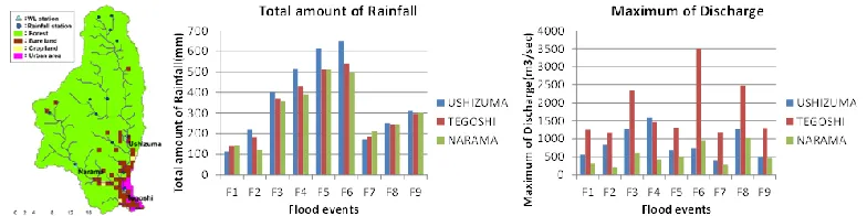
The target basin of this study is the Abe River basin in Japan, with a basin area of 567.0 km2. The left of Figure 1 shows a map of the target basin which includes the configuration of thirteen rainfall stations and three water level stations and the land usage information. The Abe River and the Warashina River converge and flow to the sea. Ushizuma and Narama water level stations are on the upper side of the Abe River and the Warashina River, respectively. Tegoshi water level station is below the convergence point of the two rivers. Table 1 compiles the information of the water level stations. Standby discharge for flood fighting corps and designed high discharge are used in mathematical optimization. Nine flood events are selected as the target flood events that occurred from 2005 to 2012 where the maximum of discharges exceeded 1,000 m3/s at Tegoshi.

Figure 1: The Abe River basin, total amount of rainfall and maximum of discharge

Table 1: Information of water level stations

Water level station

Basin area (m2)

Standby water level for flood fighting corps

(m)

Standby discharge for flood fighting corps (m3/s)

Designed high water level

(m)

Designed high discharge

(m3/s)

Ushizuma 288.00 2.20 355.64 5.51 4550.00

Tegoshi 537.00 1.50 138.65 4.82 5500.00

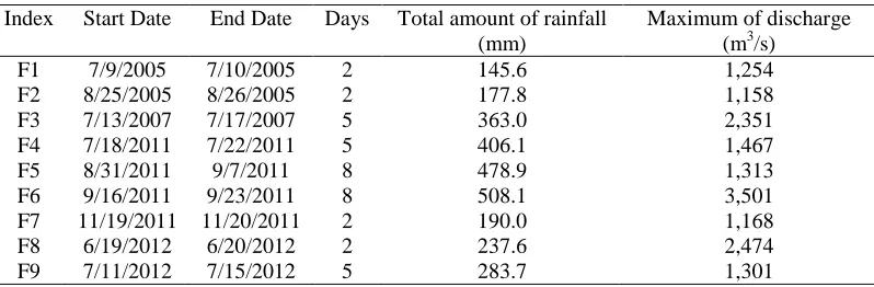
Table 2: Information of flood events

Index Start Date End Date Days Total amount of rainfall (mm)

Maximum of discharge (m3/s)

F1 7/9/2005 7/10/2005 2 145.6 1,254

F2 8/25/2005 8/26/2005 2 177.8 1,158

F3 7/13/2007 7/17/2007 5 363.0 2,351

F4 7/18/2011 7/22/2011 5 406.1 1,467

F5 8/31/2011 9/7/2011 8 478.9 1,313

F6 9/16/2011 9/23/2011 8 508.1 3,501

F7 11/19/2011 11/20/2011 2 190.0 1,168

F8 6/19/2012 6/20/2012 2 237.6 2,474

F9 7/11/2012 7/15/2012 5 283.7 1,301

The center and right of Figure 1 show the total amount of rainfall and the maximum of discharge observed at three water level stations. Statistical information of the target flood events are listed in Table 2. The characteristics of the flood events are widely different regarding when and how long the flood events occur, how much rain falls and how much discharge flows.

2.2

PWRI distributed hydrological model

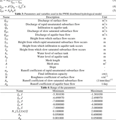
Discharge is calculated using the PWRI distributed hydrological model incorporated in an Integrated Flood Analysis System IFAS which has been developed and made publicly available by ICHARM. Figure 2 shows a schematic illustration of the PWRI distributed hydrological model. Discharge is divided and calculated as from (1) to (5). The parameters and variables used in the PWRI distributed hydrological model are presented in Table 3. To calculate the discharge, the basin is divided into 500m × 500m meshes. Two layered tanks, surface and aquifer tanks, are set up on each mesh. Four kinds of hydrological parameters are investigated as final infiltration capacity, roughness coefficient of surface flow, runoff coefficient of slow saturated subsurface flow and runoff coefficient of aquifer base flow. Five kinds of parameters are allocated depending on the land usages for final infiltration capacity and roughness coefficient of surface flow. Hence, there are twelve parameters in total. In order to investigate the relationship between parameter settings and the fitting of the discharge, 10,001 combinations of parameter sets are uniformly calculated using simplified Latin hypercube sampling in the range noted in Table 4. Thus, discharges are calculated for 10,001 combinations of parameter sets, nine flood events and three water level stations.

Figure 2: PWRI distributed hydrological model

𝑄𝑠𝑓 = 𝐿

1

𝑁(ℎ𝑠− ℎ𝑓2)

5

3_{√𝑖 (1)}

𝑄𝑟𝑖 = 𝛼𝑛𝐴𝑓0

ℎ𝑠− 𝑆𝑓1

𝑄0= 𝐴𝑓0

ℎ𝑠− 𝑆𝑓0

𝑆𝑓2− 𝑆𝑓0 (3)

𝑄𝑔1= 𝐴2(ℎ𝑔− 𝑆𝑔)

2

𝐴 (4)

𝑄𝑔2= 𝐴𝑔ℎ𝑔𝐴 (5)

Table 3: Parameters and variables used in the PWRI distributed hydrological model

Name Description Unit

𝑄𝑠𝑓 Discharge of surface flow m3/s

𝑄𝑟𝑖 Discharge of rapid unsaturated subsurface flow m3/s

𝑄0 Infiltration to aquifer tank m3/s

𝑄𝑔1 Discharge of slow saturated subsurface flow m3/s

𝑄𝑔2 Discharge of aquifer base flow m3/s

𝑆𝑓2 Height from which surface flow occurs m

𝑆𝑓1 Height from which rapid unsaturated subsurface flow occurs m

𝑆𝑓0 Height from which infiltration to aquifer tank occurs m

𝑆𝑔 Height from which slow saturated subsurface flow occurs m

ℎ𝑠 Water level of surface tank m

ℎ𝑔 Water level of aquifer tank m

𝐿 Mesh length m

𝐴 Mesh area m2

𝑖 Slope -

𝛼𝑛 Runoff coefficient of rapid unsaturated subsurface flow -

𝑓0 Final infiltration capacity cm/s

𝑁 Roughness coefficient of surface flow s/m1/3

𝐴𝑢 Runoff coefficient of slow saturated subsurface flow (1/mm/day)1/2

𝐴𝑔 Runoff coefficient of aquifer base flow 1/day

Table 4: Range of the parameters

Name Minimum Maximum

𝑓0_1 -5.301030 -1.301030

𝑓0_2 -6.698970 -2.698970

𝑓0_3 -7.000000 -3.000000

𝑓0_4 -8.000000 -4.000000

𝑓0_5 -7.000000 -3.000000

𝑁_{1,2,3,4,5} 0.100000 2.000000

𝐴𝑢 0.050000 0.600000

𝐴𝑔 0.001000 0.050000

3

Optimization method

3.1

Evaluation index score

𝑠𝑐𝑜𝑟𝑒 indicates how well observed and simulated hydrographs match. 𝑠𝑐𝑜𝑟𝑒 is calculated as the

sum of 𝑓𝑖𝑡𝑡𝑖𝑛𝑔 and 𝑝𝑒𝑛𝑎𝑙𝑡𝑦 for each parameter set, flood event and water level station. 𝑓𝑖𝑡𝑡𝑖𝑛𝑔 is calculated based on the mean squared errors normalized by the designed high discharge at the water level station and 𝑝𝑒𝑛𝑎𝑙𝑡𝑦 is calculated in order not to underestimate the duration of the flood events.

𝑓𝑖𝑡𝑡𝑖𝑛𝑔(𝑖, 𝑗, 𝑚) = 1

𝑁𝑡𝑖𝑚𝑒(𝑖)×

1

𝐷𝑒𝑠𝑖𝑔𝑛(𝑗)2× ∑ (𝑄𝑠𝑖𝑚(𝑖, 𝑗, 𝑘, 𝑚) − 𝑄𝑜𝑏𝑠(𝑖, 𝑗, 𝑘))

2 𝑁_{𝑡𝑖𝑚𝑒}(𝑖)

𝑘=1

(7)

𝑝𝑒𝑛𝑎𝑙𝑡𝑦(𝑖, 𝑗, 𝑚)

= 𝑚𝑎𝑥(𝑁𝑡𝑖𝑚𝑒_𝑜𝑏𝑠(𝑖, 𝑗) − 𝑁𝑡𝑖𝑚𝑒_𝑠𝑖𝑚(𝑖, 𝑗, 𝑚), 0) ×_𝑁 1

𝑡𝑖𝑚𝑒(𝑖)×

1

𝐷𝑒𝑠𝑖𝑔𝑛(𝑗)2

× ∑ 𝑄𝑜𝑏𝑠(𝑖, 𝑗, 𝑘)2

𝑁𝑡𝑖𝑚𝑒(𝑖)

𝑘=1

(8)

𝑁𝑡𝑖𝑚𝑒_𝑜𝑏𝑠(𝑖, 𝑗) = ∑ 1

𝑁_{𝑡𝑖𝑚𝑒}(𝑖)

𝑘=1 𝑄_𝑜𝑏𝑠(𝑖,𝑗,𝑘)≥𝑆𝑡𝑎𝑛𝑑𝑏𝑦(𝑗)

(9)

𝑁𝑡𝑖𝑚𝑒_𝑠𝑖𝑚(𝑖, 𝑗, 𝑚) = ∑ 1

𝑁𝑡𝑖𝑚𝑒(𝑖)

𝑘=1

𝑄_𝑠𝑖𝑚(𝑖,𝑗,𝑘,𝑚)≥𝑆𝑡𝑎𝑛𝑑𝑏𝑦(𝑗)

(10)

3.2

Constraint index over

𝑜𝑣𝑒𝑟 distinguishes whether each parameter set is appropriate to use for fitting and is calculated for each flood event, water level station and parameter set. Two constraint conditions are introduced to decide which simulated discharges are useful for flood fighting activities. They are 1) the maximum of the observed discharge ≤ the maximum of the simulated discharge ≤ the maximum of the observed discharge × the allowance for overestimation 𝛽 before the time for the observed discharge to reach the maximum and 2) the observed discharge ≤ the simulated discharge while the observed discharge is more or equal to the standby discharge for flood fighting corps and increases.

𝑚𝑎𝑥(𝑄𝑜𝑏𝑠(𝑖, 𝑗, 𝑘))

≤ 𝑚𝑎𝑥(𝑄𝑠𝑖𝑚(𝑖, 𝑗, 𝑘, 𝑚))

≤ 𝑚𝑎𝑥(𝑄𝑜𝑏𝑠(𝑖, 𝑗, 𝑘)) × 𝛽

𝑖 ∈ {1, … , 𝑁𝑓𝑙𝑜𝑜𝑑}

𝑗 ∈ {1, … , 𝑁𝑠𝑖𝑡𝑒}

𝑘 ∈ {1, … , 𝑇𝑚𝑎𝑥_𝑜𝑏𝑠(𝑖, 𝑗)}

𝑚 ∈ {1, … , 𝑁𝑐𝑎𝑠𝑒}

(11)

𝑄𝑜𝑏𝑠(𝑖, 𝑗, 𝑘) ≤ 𝑄𝑠𝑖𝑚(𝑖, 𝑗, 𝑘, 𝑚)

𝑖 ∈ {1, … , 𝑁𝑓𝑙𝑜𝑜𝑑}

𝑗 ∈ {1, … , 𝑁𝑠𝑖𝑡𝑒}

𝑘 ∈ {2, … , 𝑇𝑚𝑎𝑥_𝑜𝑏𝑠(𝑖, 𝑗) − 1}

𝑚 ∈ {1, … , 𝑁𝑐𝑎𝑠𝑒}

𝑄𝑜𝑏𝑠(𝑖, 𝑗, 𝑘) ≥ 𝑆𝑡𝑎𝑛𝑑𝑏𝑦(𝑗)

𝑄𝑜𝑏𝑠(𝑖, 𝑗, 𝑘 − 1) ≤ 𝑄𝑜𝑏𝑠(𝑖, 𝑗, 𝑘) ≤ 𝑄𝑜𝑏𝑠(𝑖, 𝑗, 𝑘 + 1)

(12)

3.3

Mathematical optimization

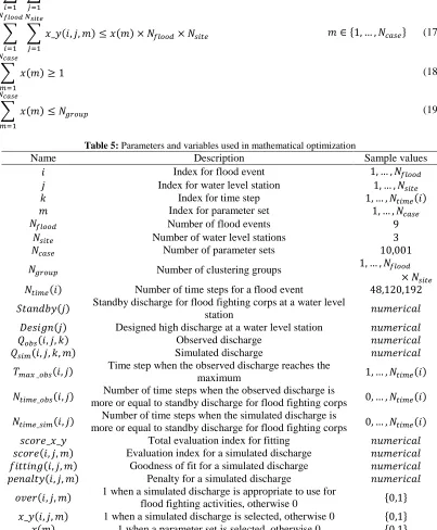
Mathematical optimization is performed to minimize the objective function (13) under the constraint conditions from (14) to (19). Table 5 describes the parameters and variables used from (13) to (19).

𝑠𝑐𝑜𝑟𝑒_𝑥_𝑦 = ∑ ∑ ∑ 𝑥_𝑦(𝑖, 𝑗, 𝑚) × 𝑠𝑐𝑜𝑟𝑒(𝑖, 𝑗, 𝑚)

𝑁𝑐𝑎𝑠𝑒

𝑚=1 𝑁_{𝑠𝑖𝑡𝑒}

𝑗=1 𝑁𝑓𝑙𝑜𝑜𝑑

𝑖=1

(13)

𝑥_𝑦(𝑖, 𝑗, 𝑚) = 𝑥_𝑦(𝑖, 𝑗, 𝑚) × 𝑜𝑣𝑒𝑟(𝑖, 𝑗, 𝑚) 𝑖 ∈ {1, … , 𝑁𝑗 ∈ {1, … , 𝑁𝑓𝑙𝑜𝑜𝑑𝑠𝑖𝑡𝑒} }

𝑚 ∈ {1, … , 𝑁𝑐𝑎𝑠𝑒}

∑ 𝑥_𝑦(𝑖, 𝑗, 𝑚) = 1

𝑁𝑐𝑎𝑠𝑒

𝑚=1

𝑖 ∈ {1, … , 𝑁𝑓𝑙𝑜𝑜𝑑}

𝑗 ∈ {1, … , 𝑁𝑠𝑖𝑡𝑒}

(15)

∑ ∑ 𝑥_𝑦(𝑖, 𝑗, 𝑚) ≥ 𝑥(𝑚)

𝑁_{𝑠𝑖𝑡𝑒}

𝑗=1 𝑁_{𝑓𝑙𝑜𝑜𝑑}

𝑖=1

𝑚 ∈ {1, … , 𝑁𝑐𝑎𝑠𝑒} (16)

∑ ∑ 𝑥_𝑦(𝑖, 𝑗, 𝑚) ≤ 𝑥(𝑚)

𝑁_{𝑠𝑖𝑡𝑒}

𝑗=1

× 𝑁𝑓𝑙𝑜𝑜𝑑× 𝑁𝑠𝑖𝑡𝑒 𝑁_{𝑓𝑙𝑜𝑜𝑑}

𝑖=1

𝑚 ∈ {1, … , 𝑁𝑐𝑎𝑠𝑒} (17)

∑ 𝑥(𝑚) ≥ 1

𝑁𝑐𝑎𝑠𝑒

𝑚=1

(18)

∑ 𝑥(𝑚)

𝑁_{𝑐𝑎𝑠𝑒}

𝑚=1

≤ 𝑁𝑔𝑟𝑜𝑢𝑝 (19)

Table 5: Parameters and variables used in mathematical optimization

Name Description Sample values

𝑖 Index for flood event 1, … , 𝑁𝑓𝑙𝑜𝑜𝑑

𝑗 Index for water level station 1, … , 𝑁𝑠𝑖𝑡𝑒

𝑘 Index for time step 1, … , 𝑁_{𝑡𝑖𝑚𝑒}(𝑖)

𝑚 Index for parameter set 1, … , 𝑁_{𝑐𝑎𝑠𝑒}

𝑁𝑓𝑙𝑜𝑜𝑑 Number of flood events 9

𝑁𝑠𝑖𝑡𝑒 Number of water level stations 3

𝑁𝑐𝑎𝑠𝑒 Number of parameter sets 10,001

𝑁𝑔𝑟𝑜𝑢𝑝 Number of clustering groups 1, … , 𝑁𝑓𝑙𝑜𝑜𝑑

× 𝑁𝑠𝑖𝑡𝑒

𝑁𝑡𝑖𝑚𝑒(𝑖) Number of time steps for a flood event 48,120,192

𝑆𝑡𝑎𝑛𝑑𝑏𝑦(𝑗) Standby discharge for flood fighting corps at a water level

station 𝑛𝑢𝑚𝑒𝑟𝑖𝑐𝑎𝑙

𝐷𝑒𝑠𝑖𝑔𝑛(𝑗) Designed high discharge at a water level station 𝑛𝑢𝑚𝑒𝑟𝑖𝑐𝑎𝑙

𝑄𝑜𝑏𝑠(𝑖, 𝑗, 𝑘) Observed discharge 𝑛𝑢𝑚𝑒𝑟𝑖𝑐𝑎𝑙

𝑄𝑠𝑖𝑚(𝑖, 𝑗, 𝑘, 𝑚) Simulated discharge 𝑛𝑢𝑚𝑒𝑟𝑖𝑐𝑎𝑙

𝑇𝑚𝑎𝑥⁡_𝑜𝑏𝑠(𝑖, 𝑗) Time step when the observed discharge reaches the _maximum 1, … , 𝑁𝑡𝑖𝑚𝑒(𝑖)

𝑁𝑡𝑖𝑚𝑒_𝑜𝑏𝑠(𝑖, 𝑗) _{more or equal to standby discharge for flood fighting corps}Number of time steps when the observed discharge is 0, … , 𝑁𝑡𝑖𝑚𝑒(𝑖)

𝑁𝑡𝑖𝑚𝑒_𝑠𝑖𝑚(𝑖, 𝑗) _{more or equal to standby discharge for flood fighting corps} Number of time steps when the simulated discharge is 0, … , 𝑁𝑡𝑖𝑚𝑒(𝑖)

𝑠𝑐𝑜𝑟𝑒_𝑥_𝑦 Total evaluation index for fitting 𝑛𝑢𝑚𝑒𝑟𝑖𝑐𝑎𝑙

𝑠𝑐𝑜𝑟𝑒(𝑖, 𝑗, 𝑚) Evaluation index for a simulated discharge 𝑛𝑢𝑚𝑒𝑟𝑖𝑐𝑎𝑙

𝑓𝑖𝑡𝑡𝑖𝑛𝑔(𝑖, 𝑗, 𝑚) Goodness of fit for a simulated discharge 𝑛𝑢𝑚𝑒𝑟𝑖𝑐𝑎𝑙

𝑝𝑒𝑛𝑎𝑙𝑡𝑦(𝑖, 𝑗, 𝑚) Penalty for a simulated discharge 𝑛𝑢𝑚𝑒𝑟𝑖𝑐𝑎𝑙

𝑜𝑣𝑒𝑟(𝑖, 𝑗, 𝑚) 1 when a simulated discharge is appropriate to use for

flood fighting activities, otherwise 0 {0,1}

𝑥_𝑦(𝑖, 𝑗, 𝑚) 1 when a simulated discharge is selected, otherwise 0 {0,1}

4

Optimization results and discussion

4.1

Number of samples which satisfy the constraint conditions

The left of Figure 3 shows the number of samples which satisfy the constraint conditions of (11) and (12). Unfortunately, no samples exist which satisfy them in the cases of the observations for F4 at Ushizuma, for F5 at all the water level stations and for F6 at Narama. For these cases, 1 is set to the constraint index 𝑜𝑣𝑒𝑟(𝑖, 𝑗, 𝑚) and mathematical optimization is performed to minimize the objective function regardless of the constraint conditions.

Figure 3: Number of satisfactory samples and number of necessary clustering groups

4.2

Relationship between the allowance of overestimation and the

number of clusters

The right of Figure 3 shows the relationship between the allowance of overestimation 𝛽 and the number of clustering groups 𝑁𝑔𝑟𝑜𝑢𝑝. 𝛽 and 𝑁𝑔𝑟𝑜𝑢𝑝 are arranged in horizontal and vertical directions, respectively. Red and blue cells correspond to whether the combinations of parameter sets satisfy all the constraint conditions. A natural result is shown that the decrease of 𝛽 causes the increase of

𝑁𝑔𝑟𝑜𝑢𝑝. Although accuracy to estimate the discharge is required for appropriate flood fighting activities, it is difficult to simulate the discharge accurately. For example, 1.2 is selected for 𝛽 in consideration of the balance of the requirement and difficulty, which is a twenty percent overestimation of the maximum discharge allowed. The optimization result reveals that eight combinations of parameter sets are necessary to estimate twenty-seven hydrographs to minimize the objective function under the constraint conditions.

4.3

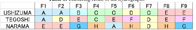
Clustering of the hydrographs

Table 6 shows the optimization result. Eight combinations of parameter sets are selected by mathematical optimization, which are noted from A to H. Flood events and water level stations are arranged in columns and rows, respectively. Each of the twenty-seven cells corresponds to each of the twenty-seven hydrographs. Parameter set E estimates seven out of twenty-seven hydrographs and is recognized as the most common among 10,001 candidates. Parameter set B only appears in the cell of F3 and Ushizuma, which is selected to describe specific characteristics of the water level station and the flood event. Parameter set F only appears in Tegoshi and parameter sets G and H only appear in Narama, which are selected to describe the specific characteristics of the water level stations.

4.4

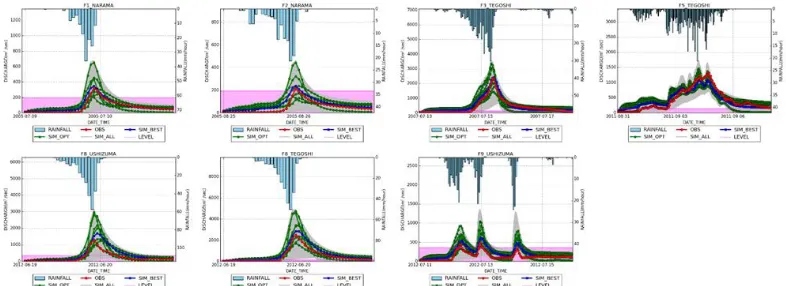
Fitting of hydrographs

Figure 4 shows the fitting of the hydrographs in the case of the most common parameter set E. RAINFALL, OBS, SIM_BEST, SIM_OPT, SIM_ALL and LEVEL show rainfall, the observed discharge, the simulated discharge estimated with the parameter set E which minimize the objective function, the simulated discharges estimated with eight combinations of parameter sets from A to H, which indicates the range of the discharges that are supposed based on nine flood events, the simulated discharge estimated with 10,001 combinations of parameter sets which indicate the range of the discharges that the PWRI distributed hydrological model may simulate, and the standby discharge for flood fighting corps.

Figure 4: Fitting of the hydrographs for the parameter set E.

5

Conclusion

A mathematical optimization procedure was presented to make clusters of multiple hydrographs simulated with a distributed hydrological model, where a different parameter set is selected for each cluster and the hydrographs belonging to each cluster are estimated with the corresponding parameter set. An optimization result demonstrates that eight parameter sets are necessary to describe twenty-seven hydrographs observed in nine flood events and at three water level stations in the Abe River basin in Japan. Thus, the parameter sets obtained by mathematical optimization help the comprehensive understanding of various flood events in the basin.

References

[1] Qingyun Duan, Soroosh Sorooshian, Vijai Gupta, Effective and efficient global optimization for conceptual rainfall-runoff models, Water Resources Research, Vol.28, No.4 (1992) 1015-1031. [2] Patrice Ogou Yapo, Hoshin Vijai Gupta, Soroosh Sorooshian, Multi-objective global

optimization for hydrologic models, Journal of Hydrology, Vol.204 (1998) 83-97.

[3] Seong Jin Noh, Yasuto Tachikawa, Michiharu Shiiba, Kazuaki Yorozu, Sunmin Kim, Development of a hydrological modeling framework for data assimilation with particle filters, Journal of JSCE, Vol.1 (2013) 69-81.