Volume 7, 2018, Pages 50–67
PROOFS 2018. 7th International Workshop on Security Proofs for Embedded Systems
A Non-Reversible Insertion Method for Hardware Trojans
Based on Path Delay Faults
Akira Ito, Rei Ueno, Naofumi Homma, and Takafumi Aoki
Tohoku University, Sendai, Miyagi, Japan
{ito, ueno, homma}@riec.tohoku.ac.jp, [email protected]
Abstract
This paper presents a non-reversible method for stealthily inserting hardware Tro-jan (HT) based on a path delay fault called Path Delay HT (PDHT). While PDHT is hardly detected by the conventional methods including Monte-Carlo tests, its practicality is still unclear because a rarely sensitized path used for PDHT is selected and exploited in a deterministic manner. Such deterministic method indicates that we can find possible PDHT-inserted paths by its reversed method. In addition, the conventional method uses a genetic algorithm to add extra delays onto the selected path for inducing a path delay fault, and therefore, we have a difficulty in evaluating the resistance/vulnerability of a circuit to PDHT. This paper first presents a new method for selecting sufficiently rare paths to insert PDHT at random. We then show that the detectability/stealthiness of PDHT is related to switching activity (i.e., glitch effect), and present a new systematic method for inducing a path delay fault instead of GA. We demonstrate through an experimental PDHT-insertion and a Monte-Carlo test that the PDHT inserted by our method is sufficiently undetectable in comparison with the conventional method.
1
Introduction
Threats from hardware Trojans (HTs), which behave as hardware-oriented backdoors intro-ducing faults or leaking out secret information, have gained increasing attention in academia, industry, and government agencies. HTs can be inserted by many involved companies (e.g. fabless companies, design houses, IP vendors, and semiconductor foundries) throughout the production process. In particular, malicious parties can introduce an HT into cryptographic hardware in order to retrieve secret information from the chip users and/or their clients.
There are many previous works related to HT detection mechanisms and countermeasures. Conventional HTs usually modify the functionality of target circuits at the register transfer level (RTL), net-list level, layout-level, or dopant-level in order to obtain secret information directly, to induce a fault for differential fault analysis (DFA), or to disable/degrade an embedded (pseudo) random number generator [1, 2, 3, 4]. Because these approaches should necessarily change the physical characteristics and/or the structures of the circuit, many countermeasures have been reported to detect such HTs. For example, we can examine side-channel information (e.g., power consumption) or compare a scanning electronic microscope (SEM) image of a chip layout with the reference.
In recent years, however, a new type of HT, called path delay HT (PDHT), was proposed at CHES 2016 [5]. A PDHT is inserted to a multiplier used for public key cryptographic hardware (e.g., RSA and ECC) to retrieve a secret key using the bug attack [6]. Such PDHT is inserted only by increasing the delay of a rarely sensitized path called rare path (RP). The PDHT can be triggered by applying a specific input sensitizing the RP to the HT-inserted multiplier. The propagation delay along the RP is larger than the original clock period, and therefore a setup time violation occurs when the RP is sensitized, which results in a buggy output. Only one buggy output of the multiplier is enough for the bug attack to retrieve the secret key of ECC and RSA. A PDHT is inserted without modifying the circuit function (i.e., input-output relation), datapath, nor structure in contrast to the conventional HTs. Furthermore, according to [5], the increase of a logic gate delay can be done with minor change in appearance or physical characteristics (e.g., cell size and power consumption), even in comparison with a dopant-level HT. As a result, it is very difficult to detect the PDHT using the conventional detection methods such as reverse-engineering, visual inspection, side-channel profiling, and SEM scanning.
However, the generality and practicality of PDHT are still unclear because of some questions about the resistance (i.e., stealthiness/detectability) of PDHTs in multipliers. The PDHT-insertion consists of two phases: (a) RP selection and (b) delay addition. The RP selection phase finds an RP in a multiplier in accordance with two features of each gate: controllability and observability. The delay addition phase determines the amount of extra delay for each gate along the selected RP in order to minimize the probability of setup time violation (i.e., the possibility of PDHT detection) during chip test via the Monte Carlo method. Here, the RP selection method in [5] selects only one RP in a deterministic manner. This means that we can reversely find the RP using the same selection method. In addition, the delay addition is performed using a genetic algorithm (GA). This indicates that we encounter a difficulty in evaluating its stealthiness and effectiveness in an analytic manner because of the irreproducibility and large processing time of GA. In particular, a time-consuming Monte-Carlo-based method would be required to determine the fitness function in GA, which has a significant impact on the resulting stealthiness/detectability in the context of PDHD.
This paper presents the possibility of inserting PDHTs in a non-reversible manner and ana-lyzing the PDHT stealthiness and effectiveness. We first formulate the sensitization probability of a path using switching activity (i.e., glitches), while the previous paper did not mention the relation between the sensitization probability and glitches. Thereafter, we define a new metric, which is called gate switching detectability, to derive the sensitization probability of a path according to path features including glitches effects. Our approach makes it possible to discuss how much a path is undetectable if a PDHT is inserted. In addition, we present a system-atic delay addition method that offers comparable stealthiness to the conventional GA-based method. In an example of an experimentally PDHT-inserted multiplier, the proposed method achieves an equivalent detection probability against the Monte-Carlo test. The result shows that the PDHT inserted by the proposed method is hardly detected by its reversed method and can be a practical threat to public key cryptographic hardware.
2
Previous work
to be hardly sensitized, only attacker who knows how to activate the path can obtain the faulty output available for the bug attack owing to the setup time violation. Therefore, reducing the sensitization probability of HT-inserted path is quite important. If the sensitization probability is high, the PDHT can be detected via a typical Monte-Carlo test in quality check after chip fabrication. In practice, it is not simple to reduce the detection probability of PDHT because a path delay fault can be detected even when the path is partially sensitized. This indicates that the extra delay for PDHT should be added to each gate along RP such that its influence on other paths is minimum. To address the purpose, the PDHT-insertion method in [5] consists of RP selection and delay addition phases to reduce the detection probability. We briefly describe the two phases below.
2.1
Rare path selection
This phase selects the most rarely sensitized path in a multiplier in accordance with two features of gates: controllability and observability. Controllability is a probability of the gate output (i.e., a wire) for “1” when a random vector is applied to the multiplier. Observability is a probability that the value of gate output can be observed from the primary output of the circuit. A low observability of a gate indicates that its output value is unlikely to propagate to the primary output. Therefore, from the viewpoint of detectability, it is better to insert PDHT to a path with low controllability and observability. Controllability and observability are the metrics focusing on the static state of a circuit, which indicates that all gate switchings are completed after applying an input vector. In other words, they are calculated without considering glitch effects, and can be calculated from a logical expression (or gate-level netlist) of the multiplier. However, it is infeasible to calculate the exact controllability of each gate for practical multipliers even with the state-of-the-art SAT solvers. Therefore, in practice, controllability and observability are asymptotically calculated using a Monte-Carlo test.
In the path selection presented in [5], we first find a gate with the lowest controllability. We then extend a path from the gate to a primary input wire and output wire according to controllability and observability. This method selects gates such that its output is the most uncontrollable and unobservable among candidates. Finally, the SAT solver is used for examining whether the path is logically sensitizable. Thus, the attacker can select a rarely sensitized path and determine the input vectors to sensitize it.
However, the above method selects only one path in a deterministic manner. This means that we can reversibly find the path for PDHT using the same method and eventually detect the PDHT, while the path is usually not detected with Monte-Carlo tests. This implies the impracticality of PDHT. To show that PDHT can be a practical threat to cryptographic hard-ware, we should show a possibility of a non-reversible method that can randomly insert PDHT with a low detectability. Note here that it is still not sufficient to randomly select an initial gate with a low controllability under a threshold though it increases RP candidates by only the number of candidates for initial gates. In other words, we should randomly select a path with a low sensitizability rather than initial gates. However, it should be noted that if we select a path in a completely random manner, we can detect PDHT by Monte-Carlo tests [8].
2.2
Delay addition
determine the increase of RP delay. GA is an optimization technique that (locally) minimizes a cost function called the fitness function. We need to give some constraints on gate delays and determine the fitness function in order to apply GA to inserting extra delays on the RP. In [5], the fitness function is given by Monte Carlo tests, and the constraints on delays for each gate is given by
t0RP = n
X
i=0
t0ζ, (1)
tζ+υζ−c≤tζ0 ≤tζ +υζ+c, (2)
wheret0RP is the resulting RP delay,υζ is a slack of theζthgate, andcis a constant. The slack represents a possible range of delay, and the constantclocalizes the solution of GA for efficient computation. In addition,tζ andt0ζ are the delays of the original and resultingithgate on RP, respectively. The first equation indicates that the resulting RP delay should be equal to the target delayt0RP which exceeds the original critical delay (i.e., clock period), while the second equation helps the GA to discover reasonable delays for each gate. The slack for each gate is determined according to the delay of the gate, data dependency, and the clock period [9].
There are several issues involved in using GA in the context of PDHT. One is that GA usually takes a huge computation time. To make the resolution of detectability sufficiently low, a large number of random vectors are required for the fitness function, which implies a significant amount of time to evaluate the fitness function. In addition, large numbers of generations and individuals (each of which requires an evaluation of the fitness function) are necessary to obtain a good solution in GA. Thus, delay addition for a PDHT is quite time-consuming, which means that it is quite difficult to analyze the detectability/stealthiness of PDHT with a statistical means. Furthermore, the usage of GA also has a problem contradicting the definition of PDHT. In evaluating the fitness function, we should apply a sufficient number of input vectors required to guarantee a low detectability. In other words, because we should detect PDHT to evaluate the fitness function, the number of input vectors should be never enough to ensure that the PDHT is significantly undetectable. This problem originates from the difficulty in evaluating the quality of a solution in GA in a quantitative manner. Thus, it is difficult to evaluate and compare the detectability/stealthiness of PDHT in many multipliers in an analytical and quantitative manner because of the usage of GA, which makes difficult to develop multipliers robust to PDHT. To develop countermeasures, a more systematic/analytical method for delay addition is desirable.
3
Gate Switching Detectability (GSD)
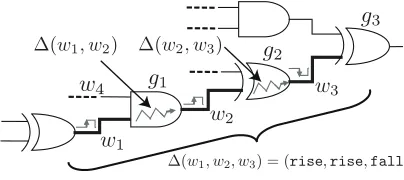
Figure 1: Circuit example.
3.1
Notations for path sensitization probability
This subsection introduces mathematical notations to represent the path sensitization proba-bility in a formal manner. Figure1 shows an example of circuit. We model a circuit as sets of Wires. Gates, and paths are then represented with wires. The notations for wire, gate, and path are as follows.
3.1.1 Wire
A circuit represented with wires w1, w2, . . . , wu, . . . , we, where e is the number of wires. We call the signal transition of 0→1 and 1→0 on a wirerise andfall, respectively. Let ∆wu be the signal transition on wirewu. The transitions of rise andfall on wu are denoted by ∆wu=riseand ∆wu=fall, respectively. The notations for wires and their signal transitions are listed below.
• w1, w2, . . . , wu, . . . , we: a wire in the circuit, whereeis the number of wires in the circuit.
• rise: the transition from 0 to 1. • fall: the transition from 1 to 0.
• null: no transition (i.e., transitions from 0 to 0 and from 1 to 1).
• ∆wu: Transition of a signal on wirewu. A rising and falling transition ofwuare denoted by ∆wu = rise and ∆wu = fall, respectively. No transition of wu is denoted by ∆wu=null
• W: the set of all wires in the circuit.
• WPI: the set of all wires connected directly from the primary input(s).
• WPO: the set of all wires connected directly to the primary output(s).
• Srfn={rise,fall,null}: the set of signal transitions. • Srf={rise,fall}: the set of signal switching.
• su∈ Srfn: variable of signal transitions for ∆wu.
• σu∈ Srf: variable of signal switchings for ∆wu
3.1.2 Gate
Gatesg1, g2, . . . , gi, . . . , gm are given as the pairs of the set of input wires and a output wire, wheremis the number of gates.
• gi = (Wgi, wi): a logic gate, where Wgi denotes the set of input wires connected to gi,
and wi denotes the output wire of gi. For a d-input gate gi, Wgi consists of d wires
wi1, wi2, . . . , wih, . . . , wid. Note that a gategicorresponds to the output wirewi because
we assume here that every logic gate has only one output, without loss of generality1.
• G: the set of all gates in the circuit.
• WPRE(wi) = {wt | gi = (Wgi, wi) ∈ G, wt ∈ Wgi}: the set of wires given from the
predecessor ofwi.
• WSUC(wi) ={wf |gf = (Wgf, wf)∈ G, wi∈ Wgf}: set of wires of successor ofwi.
For example, in Fig. 1, g1 is given as (Wg1, w2), where Wg1 ={w1, w4} and w2 is an output
wire.
3.1.3 Path
Paths are given as tuples of wires connected via gates from an input to an output. A series of signal transitions throughout a path is calledpath sensitization (state). The notations for path and path sensitization are listed below.
• p= (wv1, wv2, . . . , wvj, . . . , wvl): a path through l wires wv1, wv2, . . . , wvl, wherevj is an
integer in the range of 1 ≤ vj ≤ e. In addition, wv1 and wvl are the startpoint and
endpoint wires, respectively.
• |p|: the length (i.e., the number of wires) ofp. Note here that a wirewv1 corresponds to
a path with|(wv1)|= 1.
• Head(p): the startpoint wire ofp(i.e.,wv1).
• Tail(p): the endpoint closest ofp(i.e.,wvl).
• P: the set of all paths in the circuit.
• PWH,WT ={p|p∈ P,Head(p)∈ WH,Tail(p)∈ WT}: the set of paths from Head(p)∈
WHto Tail(p)∈ WT, where WHandWTare an arbitrary subset ofW.
• ∆p= ∆(wv1, wv2, . . . , wvl) = (σv1, σv2, . . . , σvl): path sensitization state (i.e., propagation
of signal transitions).
• ∆Psub = [
px∈Psub
{∆px = (σx1, σx2, . . . , σx|px|) |(σx1, σx2, . . . , σx|px|) ∈ S
|px|
rf }: the set of
possible sensitization states of all paths in Psub excluding ones containing null wires, wherePsub denotes a subset ofP. Note that elements of ∆Psub are given in the form of ∆px= (σx1, σx2, . . . , σx|px|).
1We can discuss multi-output gates (e.g., full adder cell) as plural gates with only one output. For example,
For example, in Fig. 1, pex = (w1, w2, w3) is a path, and ∆pex = ∆(w1, w2, w3) = (rise,rise,fall) indicates the path sensitization state that the rise transition of the sig-nal onw1 causes therisetransition of the signal onw2and finally causes thefalltransition of the signal onw3.
3.2
Formula for path sensitization probability between inputs and
output of each gate
We now focus on the sensitization probability of a path. Let Pr(A) be the probability of event (i.e., occuring transition(s))A. From the above notation, given a path p= (wv1, . . . , wvl), its
transition is represented by ∆p= (∆wv1, . . . ,∆wvl). Hence, the sensitization probability ofpis
represented by Pr(∆p= (σv1, . . . , σvl)). However, we cannot compute the sensitization
proba-bility because the relation between the switching probaproba-bility of each wire and the sensitization probability of a path is unclear. Therefore, let us consider the simplest case where a signal switching of an input wire propagates to the output of a gate. Letgi= (Wgi, wi) be ad-input
gate, wherewi1, . . . wih, . . . wid ∈ WPRE(wi). Using the probability marginalization, the signal
transition probability ofwi is given by
Pr(∆wi=σi) =
X
(si1,...,sid)∈Srfnd
Pr(∆wi=σi,∆wi1 =si1, . . . ,∆wid=sid). (3)
Here, we assume that two (or more) input signals never propagate to the gate output simulta-neously, because it is physically impossible for two (or more) events to occur at completely at the same time in the real world2. In other words, at most only one input signal is either rising or falling at a moment. Hence, Eq.3 is simplified as follows:
Pr(∆wi=σi) = Pr(∆wi=σi,∆wi1 =rise,∆wi2 =null, . . . ,∆wid=null)
+ Pr(∆wi=σi,∆wi1 =fall,∆wi2 =null, . . . ,∆wid=null)
+ Pr(∆wi=σi,∆wi1 =null,∆wi2 =rise, . . . ,∆wid=null)
+ Pr(∆wi=σi,∆wi1 =null,∆wi2 =fall, . . . ,∆wid=null)
.. .
+ Pr(∆wi=σi,∆wi1 =null,∆wi2 =null, . . . ,∆wid=rise)
+ Pr(∆wi=σi,∆wi1=null,∆wi2 =null, . . . ,∆wid=fall). (4)
In Eq.4, each term on the right side can be considered as the sensitization probability of a path consisting of an input and output wire of the gate. Therefore, we can confirm the relation:
Pr(∆wi=σi,∆wih =σih,∆wi1 =null, . . . ,∆wih−1 =null,
∆wih+1=null, . . . ,∆wid=null) = Pr(∆(wih, wi) = (σih, σi)). (5)
Using Eq.5, we can derive
Pr(∆wi=σi) =
X
wih∈Wgi
X
σih∈Srf
Pr(∆(wih, wi) = (σih, σi)). (6)
2 In fact, modern EDA tools for generating SAIF assume that signals of two or more input wires never
Eq. 6 indicates the relation between the switching probability of the gate output and the sensitization probability of each path from an input to the output of the gate.
Now let us consider the probability of a specific transition propagating through the gate represented by Pr(∆wi =σi,∆wih =σih). Using a probability marginalization similar to the
above, the sensitization probability Pr(∆wi=σi,∆wih =σih) is transformed to
Pr(∆wi=σi,∆wih=σih)
= X
(si1,...,sih−1,sih+1,...sid)∈S d−1
rfn
Pr(∆wi =σi,∆wih =σih,∆wi1 =si1, . . . ,∆wih−1 =sih−1,
∆wih+1=sih+1, . . . ,∆wid=sid)
= Pr(∆wi=σi,∆wih=σih,∆wi1=null, . . . ,∆wih−1 =null,
∆wih+1=null, . . . ,∆wid=null).
= Pr(∆(wih, wi) = (σih, σi)) (7)
Eq. 7 indicates the sensitization probability of a path from input to output of the gate is equal to the simultaneous probability of a signal switchings of input and output wires. In next subsection, we consider the sensitization probability of a path of which length is more than 2 using the above relation.
3.3
Calculation of path sensitization probability
This subsection formulates the sensitization probability of a path of which length is more than 2. The switching activity of each wire and each gate is derived from gate-level timing simulation because modern EDA tools (e.g., VCS and NcVerilog) can record transitions of wires and paths from an input to the output of each gate as switching activity information file (SAIF). For example, when the number ofrisetransitions of a wiren∆wi=rise is recorded as the switching
activity in SAIF, the rise transition probability of the wire is given as ∆t/T ×n∆wi=rise,
where ∆tis therise transition delay of the wire andT is simulation time that elapses in the timing simulation to obtain the switching activities. Since in this paper we assume that ∆t
of all wires are same, the transition probability of each wire has a factor of ∆t/T. Therefore, GSD mentioned later must have the same factor, too. However, it doesn’t matter whether the exact value of ∆t/T can be obtained because only the magnitude relationship between GSDs of gates plays an important role in the PDHT-insertion. Thus, when we calculate the transition probability of each wire, the ∆t/T can be practically ignored.
conditional probability of path sensitization as follows:
Pr(∆pex= (rise,rise,fall))≈Pr(∆w3=fall|∆w2=rise)Pr(∆w1=rise,∆w2=rise) = Pr(∆w2=rise,∆w3=fall)
Pr(∆w2=rise)
Pr(∆w1=rise,∆w2=rise). (8)
Note that Pr(A|B) = Pr(A, B)/Pr(B). Because Pr(∆w2=fall,∆w3=rise) and Pr(∆w1=
rise,∆w2=rise) and Pr(∆w2=rise) are derived from SAIF, we can calculate the sensiti-zation probability Pr(∆pex= (rise,rise,fall)). Using Eq.7, we derive
Pr(∆pex= (rise,rise,fall))≈
Pr(∆(w1, w2) = (rise,rise))Pr(∆(w2, w3) = (rise,fall)) Pr(∆w2=rise)
.
(9) Eq. 9 indicates that the sensitization probability with length of more than 2 is approximated by the sensitization probabilities of paths with length of up to 2.
We then generalize Eq. 8 to arbitrary path p = (wv1, . . . , wvl) with length of more than
3. Along with Eq. 8, the path sensitizability Pr(∆p = (σv1, . . . , σvl)) is decomposed to the
products of conditional and simultaneous probabilities as follows:
Pr(∆p= (σv1, . . . , σvl))≈Pr(∆wv1=σv1)
|p|
Y
j=2
Pr(∆wvj =σvj|∆wvj−1 =σvj−1)
= Pr(∆wv1=σv1)
|p|
Y
j=2
Pr(∆wvj =σvj,∆wvj−1 =σvj−1)
Pr(∆wvj−1 =σvj−1)
. (10)
Because the terms at the right hand side of Eq.10are given only by switching activity of each wire and each gate on pathp(i.e., Pr(∆wvj−1 =σvj−1) and Pr(∆wvj =σvj,∆wvj−1 =σvj−1))
we can calculate a path sensitization probability from an SAIF according to Eq.10. In addition, we can efficiently compute the sum of the sensitization probabilities of paths required for GSD using Eq. 10, as described in Sect. 3.4.
3.4
Formulation and efficient computation of GSD
Using the notation in Sect. 3.1, we define GSD (denoted byγ) as a sum of sensitization prob-abilities of all paths between a primary input and output through gi, which represents the influence ofgi on PDHT detection.
Definition 1. γgi,wih(σih, σi), which is the GSD ofgi= (Wgi, wi)on an input wirewih ∈ Wgi
forσih andσi, is defined as
γgi,wih(σih, σi)
= X
∆py∈∆PWPI,PPRE (wih)
X
∆pz∈∆PWSUC (wi),WPO
Pr(∆(wy1, . . . , wy|py|, wih, wi,
wz1, . . . , wz|pz|) = (σy1, . . . , σy|py|, σih, σi, σz1, . . . , σz|pz|)), (11)
wherepy= (wy1, wy2, . . . , wy|py|)andpz= (wz1, wz2, . . . , wz|pz|). Note here thatwy1 andwz|pz|
should be a wire of respectively primary input and output, and(wy1, . . . wy|py|, wih, wi, wz1, . . . ,
Note also that a d-input gate has 4d GSDs on input wires wi0, wi1, . . . , wih, . . . , wid for
σih∈ {rise,fall}andσi∈ {rise,fall}. This definition originates the fact that the modern
EDA tools define gate switching as a propagation of signal transition from an input wire to the output wire.
In the following, according to Eq.10, we transform the GSD in Eq.11into a form that can be efficiently computed. Using Eq.10, we can rewrite the above GSD as follows:
γgi,wih(σih, σi) =
Pr(∆(wih, wi) = (σih, σi))
Pr(∆wih=σih)
× X
∆py∈∆PWPI,WPRE (wi
h)
Pr(∆(wy1, . . . , wy|py|, wih) = (σy1, . . . , σy|py|, σih))
× X
∆pz∈∆PWSUC (wi),WPO
Pr(∆(wi, wz1, . . . , wz|pz|) = (σi, σz1, . . . , σz|pz|))
Pr(∆wi=σi)
. (12)
On the right hand side of Eq.12, the termP
∆pyPr(∆(wy1, . . . , wy|py|, wih) = (σy1, . . . , σy|py|,
σih)) represents the sum of the sensitization probabilities of all paths from the primary input
to wih, and the term Pr(∆(wi, wz1, . . . , wz|pz|) = (σi, σz1, . . . , σz|pz|)) represents that of paths
fromwi to primary output. In other words, the former and later terms are the controllability and observability, considering dynamic hazard (i.e., glitch effect), respectively. We name them dynamic controllabilityonwih forσih anddynamic observabilityonwiforσi, which are denoted
by DyConw
ih(σih) and DyObwi(σi), respectively.
Using Eq.12, we introduce Lemma 1 for efficient computation of dynamic controllability.
Lemma 1. Given a wire wih, the dynamic controllability is computed as the switching
proba-bility of signal onwih as follows:
DyConw
ih(σih) = Pr(∆wih =σih). (13)
Similarly, for the dynamic controllability, we then introduce Lemma 2 below on the efficient computation of dynamic observability.
Lemma 2. Given a wire wi, DyObwi(σi) can be computed from the dynamic observability of
its successive wirewi0 recursively as follows:
DyObw
i(σi) =
X
wi0∈WSUC(wi)
X
σi0∈Srf
Pr(∆wi0 =σi0)×DyObw
i0(σi
0)
Pr(∆wi=σi)
. (14)
Ifwi∈ WPO, thenDyObwi(σi) = 1.
Lemma 2 indicates that the dynamic observabilities can be computed iteratively from the primary output towi. See Appendices for the proofs of Lemmas 1 and 2.
Finally, GSD is represented by
γgi,wih(σih, σi) = Pr(∆(wih, wi) = (σih, σi))×DyObwi(σi). (15)
Because Pr(∆(wih, wi) = (σih, σi)), and DyOb can be computed from only SAIF according to
Algorithm 1Path Selection
Input: Circuit description (W,G,P)
Output: Rarely sensitized pathpand its sensitization state ∆p= (σv1, . . . , σvl)∈ S
|p| rf
1: parameterα; .Number of candidates (initial path seeds) for random selection
2: functionSelectRP(W,G,P)
3: setΓ ={};
4: for allgi= (Wgi, wi)∈ Gdo 5: for allwih ∈ Wgi do 6: for all(σi, σih)∈ S
2
rfdo
7: Γ←Γ ∪ {γgi,wih(σih, σi)};
8: end for
9: end for
10: end for
11: setΓα←Threshold(Γ, α); .ExtractαGSDs in order from the lowest one
12: γgini,wiini(σiini, σini)←Pick(Γα); .Determine initial path randomly 13: pathp←(wiini, wini); ∆p←(σiini, σini);
14: while Head(p)∈ W/ PI do .Extend path backward to primary input
15: setΓcand← {γgc,wic(σic, σi)|wc= Head(p), wic∈ WPRE(wc), σic∈ Srf};
16: [p,∆p]←ExtendPath(p,∆p,Γcand);
17: end while
18: while Tail(p)∈ W/ PO do .Extend path forward to primary output
19: setΓcand← {γgc,wic(σic, σc)|wic= Tail(p), wc∈ WSUC(wic), σc∈ Srf};
20: [p,∆p]←ExtendPath(p,∆p,Γcand);
21: end while
22: return[p,∆p];
23: end function
4
Proposed PDHT-insertion method
The proposed PDHT-insertion method consists of two phases: path selection and delay addition, similarly to the conventional method. Each phase of the proposed method has the following features for making PDHTs more practical and stealthy. The proposed path selection algorithm selects a path from a sufficient number of possible paths at random, which make it difficult to find the selected path by reversing the algorithm. The proposed delay addition imposes extra delay throughout the path according to the GSD values.
4.1
Path selection
Algorithm 2Path Extension
Input: Pathp, sensitization state ∆p, Set of GSDs for extension direction Γcand Output: Extended pathp0, extended sensitization state ∆p0
1: parameterρ;
2: functionExtendPath(p,∆p,Γcand)
3: floatr←rand(0,1); 4: whileΓcand6={} do
5: if r≤ρthen
6: γgc,wic(σc, σic)←MinGammaIn(Γcand); .Get lowestγ
7: else
8: γgc,wic(σc, σic)←Pick(Γcand); .Getγrandomly
9: end if
10: wirewc0 ←wcorwic;σc0←σcorσic; .Determine a wire to primary input or output
11: pathp0←ConcatPath(p, wc0); ∆p0←ConcatPathSensiState(∆p, σc0);
12: if IsSensitizable(p0, σ0) = true then
13: return[p0,∆p0];
14: else
15: Γcand←Γcand− {γgc,wic(σic, σc)}; 16: end if
17: end while
18: pathp0←RemoveGate(p); ∆p0←RemoveSensiState(∆p) .Remove the startpoint or endpoint gate
19: return[p0,∆p0]. 20: end function
Line 15, we obtain a set of candidate GSDs (i.e., wires) for extending pto a primary input. Note thatgc andσc are determined in the previous loop (or Lines 12–13 initially). At Line 16, we extend the path by choosing a candidate from Γcand using the algorithm “ExtendPath.” At Line 19, we obtain a set of candidate GSDs (i.e., wires) for extendingpto a primary output. In contrast to Line 15,gic andσic are determined in the previous loop (or Lines 12–13 initially).
At Line 20, we extend the path by choosing a candidate according to “ExtendPath” as at Line 16. Finally, at Line 22, we return a rarely sensitized path from a primary input to output and its sensitization state.
Algorithm 2 shows a function for extending a path used at Lines 16 and 20 in Alg. 1. Algorithm 2 utilizes a parameterρ∈[0,1] for randomness, in order not to detect the selected path reversely. At Line 3, we also obtain a random valuer∈[0,1]. At Lines 4–17, we determine an extension direction (i.e., a gate) for the path. Note here that we avoid simply selecting the gate with lowestγ because such PDHT is easily detected by its reverse algorithm. At Line 6, we select a candidate gate having the lowest γ ifris smaller than ρ; otherwise, at Line 8, we select a candidate gate randomly. Hence, ifρis closer to 1, we extend the path mainly based on GSD. Conversely, ifρis closer to 0, we extend the path mainly at random. Thereafter, at Line 11, we derive an extended path ofpby concatenatingpwithwc0 (i.e.,wc orwi
c), and also
derive an extended path sensitization state of ∆p. At Line 13, we return the extended path and its sensitization state after checking its sensitizability by a SAT solver becausep0 may not be sensitizable. If not sensitizable, we repeat the above process after deleting the candidate at Line 15.
Thus, we can select a rarely sensitized path with a randomness induced by αand ρ. The entropy induced byαandρis evaluated in Sect. 5.
4.2
Delay addition
detectability. Note that this delay addition can be performed in a deterministic manner in contrast to the above path selection. The delay increase of a gategj along the selected path p (denoted byτ(gj)) given by
τ(gj) =d
log2|γgj,wij(σij, σj) +|
λ
P|p|
η=1
log2|γgη,wiη(σiη, ση) +|
λ, (16)
wheredis the total delay increase of the PDHT-inserted path andwij is the input coming from
the predecessor gate on the path, and is the very small value to avoid log2(0). is needed because γgj,wij(σij, σj) becomes 0 when the transition probability of wij is recorded as 0 in
SAIF due to not enough number of applied vectors to estimate the switching activity. Because
γ varies in the exponential range (e.g.,10−12≤γ≤0.25) empirically, we use the logarithm of
γ for delay addition. In addition, because the optimal weight based on GSD depends on the structure of the multiplier, we introduce a natural numberλto optimize delay addition. The effect ofλis evaluated in the next section.
5
Experimental results
In this section, we evaluate the validity of the proposed PDHT-insertion method by an experi-mental insertion of PDHTs into a typical multiplier consisting of a partial product generator, a multiple-input adder, and a final stage adder. The target multiplier employs an AND gate array and a Wallace Tree as typical partial product generation and accumulator, respectively. On the other hand, two typical 2-input adders are used for the final stage adder: one is Ripple Carry Adder (RCA) which is the smallest and simplest, and another is Kogge Stone Adder (KSA) which is the fastest. The input bit length of the multiplier is set to 32×2 bits, which makes it difficult for functional verification and chip test in an exhaustive manner. The total delays of each selected paths varies from 1.8 to 1.2 times the critical path delay. In the evaluation,ρ
andλchange while αis set to 5.
The detection rate of the inserted PDHTs is evaluated by the Monte Carlo test, which judges the case where the operation of the multiplier was not completed within the delay of the critical path as a fault when a random vector is input. For comparison, we also evaluate the detection rate of PDHTs given from the conventional method by the same experimental setting. The
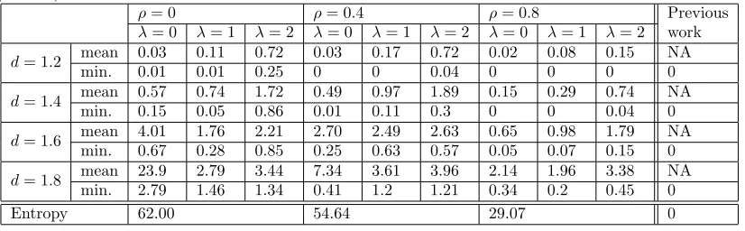
Table 1: Detectability and path entropy of PDHTs inserted into multiplier based on RCA (×10−4)
ρ= 0 ρ= 0.4 ρ= 0.8 Previous
work
λ= 0 λ= 1 λ= 2 λ= 0 λ= 1 λ= 2 λ= 0 λ= 1 λ= 2
d= 1.2 mean 0.03 0.11 0.72 0.03 0.17 0.72 0.02 0.08 0.15 NA
min. 0.01 0.01 0.25 0 0 0.04 0 0 0 0
d= 1.4 mean 0.57 0.74 1.72 0.49 0.97 1.89 0.15 0.29 0.74 NA
min. 0.15 0.05 0.86 0.01 0.11 0.3 0 0 0.04 0
d= 1.6 mean 4.01 1.76 2.21 2.70 2.49 2.63 0.65 0.98 1.79 NA
min. 0.67 0.28 0.85 0.25 0.63 0.57 0.05 0.07 0.15 0
d= 1.8 mean 23.9 2.79 3.44 7.34 3.61 3.96 2.14 1.96 3.38 NA
min. 2.79 1.46 1.34 0.41 1.2 1.21 0.34 0.2 0.45 0
parametercof the conventional method is 0.2 times the delay of the RP, or twice the minimum
cthat satisfies the constraints (1) and (2). The numbers of individuals and generations of GA are 10.
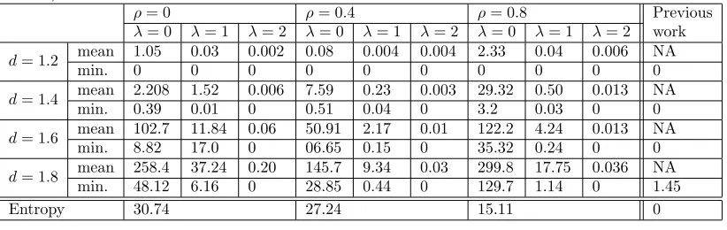
Table 1 and 2 show the detection rate of PDHTs and the entropy for the number of path candidates by the proposed method and the conventional method when RCA and KSA are used as the final stage adder, respectively. The detection rate was calculated by a Monte Carlo test with one million vectors, and it was set to 0 when detection was impossible. The first column of Tables 1 and 2 represents the magnification ratio of the added delay to the original one. Since the proposed method randomly selects a path for each trial, we performed 10 trials in the case of each condition and evaluated the detection rate of the 10 paths. Table 1 shows the lowest detection rate among the 10 paths as “min.” and the logarithmic average of the detection rates of the 10 paths as “mean”. When calculating the logarithm average, we assumed that the minimum detection rate is 10−7 in order to prevent the detection rate from being undefined.
One goal is that the detection rate required for PDHT is less than 10−6. This is because the failure rate of an large scale integration (LSI) is assumed to be about 10−6 or so. If the PDHT detection rate is less than 10−6 or less, it becomes difficult to distinguish between LSI failure and PDHT. Therefore, it is desirable that the detection rate is less than 10−6, that is “0”, in Tables 1 and 2.
In the case of a multiplier based on KSA, we can confirm that the detection rate of the proposed method decreases clearly as the value of λ is larger. Also, the detection rate is lower asρis smaller. In the case of RCA, we can find that it becomes easy to detect PDHTs by increasing the value of λ. The major reason would be that glitch is more likely to occur structurally in RCA than KSA. On the other hand, the detection rate is lower asρis larger.
Comparing the proposed method with the conventional method, we can see that the pro-posed method is better or comparable for the cases of KSA and the conventional method is better for the cases of RCA. Note however that since the conventional method select only one path in a deterministic manner, the path can be easily detected by the same method as the insertion. On the other hand, the proposed method can prevent the inserted PDHT from being detected by the same method due to the random selection of the path.
In the proposed method, the entropy of the path candidate is determined by the values of
αandρ. The entropy in Tables 1 and 2 are calculated as follows. First, let the average number of gates included in the selected path beE[|p|]−1. Here, assuming 2 input gates, we select
gates on the basis of GSD preferentially with probabilityρand randomly select with probability
Table 2: Detectability and path entropy of PDHTs inserted into multiplier based on KSA (×10−4)
ρ= 0 ρ= 0.4 ρ= 0.8 Previous
work
λ= 0 λ= 1 λ= 2 λ= 0 λ= 1 λ= 2 λ= 0 λ= 1 λ= 2
d= 1.2 mean 1.05 0.03 0.002 0.08 0.004 0.004 2.33 0.04 0.006 NA
min. 0 0 0 0 0 0 0 0 0 0
d= 1.4 mean 2.208 1.52 0.006 7.59 0.23 0.003 29.32 0.50 0.013 NA
min. 0.39 0.01 0 0.51 0.04 0 3.2 0.03 0 0
d= 1.6 mean 102.7 11.84 0.06 50.91 2.17 0.01 122.2 4.24 0.013 NA
min. 8.82 17.0 0 06.65 0.15 0 35.32 0.24 0 0
d= 1.8 mean 258.4 37.24 0.20 145.7 9.34 0.03 299.8 17.75 0.036 NA
min. 48.12 6.16 0 28.85 0.44 0 129.7 1.14 0 1.45
1−ρ. This is equivalent to selecting a gate of the lower GSD with probability (1 +ρ)/2, and selecting another gate with probability (1−ρ)/2. In the path selection, this gate selection can be considered to repeat by the average number of gates. Therefore, the average entropyH(ρ)
is given as
H(ρ) =E[|p| −1]
2
(1 +ρ) log2 1 +ρ
2 + (1−ρ) log2 1−ρ
2
. (17)
Whenρis 0, the entropy for the number of candidates is equal to the exponent part to represent the number of possible paths. In this experiment, the numbers of possible paths from a selected gate in KSA and RCA are about 230 and 260, respectively. The values of
E[|p| −1] are then
estimated to be roughly 30 and 60 for KSA and RCA, respectively. In addition, if the number of candidate paths does not heavily change depending on the selected gate, we can simply add log2(α) to Eq.17for calculating the entropy which increases by the number of seeds for the path selectionα. In fact, we confirmed that the number of candidate paths did not change much depending on experimentally selected gates. The results of Tables 1 and 2 were given by the above calculation. At a first glance, it seems that the entropy of the number of path candidates is small. However, for all these candidate paths, it is necessary to investigate a possible input to sensitize the path with a SAT solver. Since the time taken by a SAT solver was about from 0.5 seconds to several ten minutes experimentally, it is difficult to examine all the candidate paths with a realistic time if the entropy becomes about 20. Therefore, the PDHT inserted by the proposed method can be a threat when the detection rate by the Monte Carlo test is less than 10−6 and the entropy is about 20. We can say that the proposed method can be a sufficiently possible threat because the above conditions are satisfied by both KSA and RCA by adjusting the parameters.
6
Conclusion
This paper presented a non-reversible insertion method of PDHTs. First, we theoretically analyzed the relation between switching activity and path sensitization probability, and derive a new metric named Gate Switching Detectability (GSD) in order to evaluate the effect of the delay added to a logic gate on the whole circuit. Then, we proposed a new PDHT-insertion method consisting of a non-reversible path selection method and a delay addition method based on GSD. Unlike the conventional method based on the deterministic method, the proposed method has the feature that makes it difficult to detect PDHTs by tracing the insertion method. Furthermore, through the Monte Carlo test on multipliers with PDHT inserted by the proposed method and the conventional inserted, we confirmed that the proposed PDHT-insertion method could be a threat in practice.
In the future, a more detailed evaluation of PDHT detection rates would be required, and effective countermeasure/detection method for PDHTs should be studied.
Acknowledgment
References
[1] Matthew Hicks, Murph Finnicum, Samuel T King, Milo MK Martin, and Jonathan M Smith. Over-coming an untrusted computing base: Detecting and removing malicious hardware automatically. InSecurity and Privacy (SP), 2010 IEEE Symposium on, pages 159–172. IEEE, 2010.
[2] Eli Biham and Adi Shamir. Differential fault analysis of secret key cryptosystems. Advances in Cryptology—CRYPTO, pages 513–525, 1997.
[3] Raghavan Kumar, Philipp Jovanovic, Wayne Burleson, and Ilia Polian. Parametric trojans for fault-injection attacks on cryptographic hardware. In Fault Diagnosis and Tolerance in Cryptography (FDTC), 2014 Workshop on, pages 18–28. IEEE, 2014.
[4] Georg T Becker, Francesco Regazzoni, Christof Paar, and Wayne P Burleson. Stealthy dopant-level hardware trojans. InInternational Workshop on Cryptographic Hardware and Embedded Systems, pages 197–214. Springer, 2013.
[5] Samaneh Ghandali, Georg T Becker, Daniel Holcomb, and Christof Paar. A design methodology for stealthy parametric trojans and its application to bug attacks. InInternational Conference on Cryptographic Hardware and Embedded Systems, pages 625–647. Springer, 2016.
[6] Eli Biham, Yaniv Carmeli, and Adi Shamir. Bug attacks. In Annual International Cryptology Conference, pages 221–240. Springer, 2008.
[7] Mohammad Reza Kakoee, Valeria Bertacco, and Luca Benini. At-speed distributed functional testing to detect logic and delay faults in nocs. IEEE Transactions on Computers, 63(3):703–717, 2014.
[8] Akira Ito, Rei Ueno, Naofumi Homma, and Takafumi Aoki. On the detectability of hardware trojans embedded in parallel multipliers. In IEEE International Symposium on Multiple-Valued Logic (ISMVL), Linz, Austria, 2018.
[9] Xiaoyong Tang, Hai Zhou, and Prith Banerjee. Leakage power optimization with dual-v th library in high-level synthesis. InProceedings of the 42nd annual Design Automation Conference, pages 202–207. ACM, 2005.
A
Proof of Lemma 1
Lemma 1. Given a wire wih, the dynamic controllability is computed as the switching
proba-bility of signal onwih as follows:
DyConw
ih(σih) = Pr(∆wih =σih). (18)
Proof. Let ξ(wih) be the longest path length among paths from the primary input to wih,
namely,
ξ(wih) =p max y∈PWPI,WPRE (wi
h)
|py|. (19)
Prove Lemma 1 using mathematical induction. Let Q(k) be the statement of Lemma 1 where
k=ξ(wih).
We observe that Q(2) is true from Eq.6.
have
DyConw
ih(σih)
= X
∆py∈∆PWPI,WPRE (wih)
Pr(∆(wy1, . . . , wy|py|, wih) = (σy1, . . . , σy|py|, σih))
= X
∆py∈∆PWPI,WPRE (wih)
Pr(∆py= (σy1, . . . , σy|py|))
Pr(∆wy|py| =σy|py|)
×Pr(∆(wy|py|, wih) = (σy|py|, σih))
= X
wi0
h0
∈WPRE(wih)
X
σi0
h0
∈Srf
Pr(∆(wi0
h0, wih) = (σi
0
h0, σih))
Pr(∆wi0
h0 =σi0h0)
× X
∆py0∈∆PWPI,WPRE (wi0
h0)
Pr(∆(wy0
1, . . . , wy0|py0 |, wi 0
h0) = (σy
0
1, . . . , σy|0py0 |, σi 0
h0))
! .
(20)
Here, ifξ(wi0
h0)≤n, then Q(χ) (i.e.,
P ∆p0
yPr(∆(wy
0
1, . . . , wy
0 |py0 |, wi
0
h0) = (σy01, . . . , σy
0 |py0 |, σi
0
h0))
= Pr(∆wi0
h0 = σi
0
h0)) is true for 2 ≤ χ ≤ n. Because py
0 should be shorter than py (i.e.,
|py0|< n), we have
X
wi0
h0∈WPRE(wih)
X
σi0
h0
∈Srf
Pr(∆(wi0
h0, wih) = (σi
0
h0, σih))
Pr(∆wi0
h0 =σi0h0)
×Pr(∆wi0
h0 =σi
0
h0)
= X
wi0
h0∈WPRE(wih)
X
σi0
h0
∈Srf
Pr(∆(wi0
h0, wih) = (σi
0
h0, σih))
= Pr(∆wih =σih), (21)
according to Eq.6.
B
Proof of Lemma 2
Lemma 2. Given a wire wi, DyObwi(σi) can be computed from the dynamic observability of
its successive wirewi0 recursively as follows:
DyObwi(σi) =
X
wi0∈WSUC(wi)
X
σi0∈Srf
Pr(∆wi0 =σi0)×DyObw
i0(σi
0)
Pr(∆wi=σi)
. (22)
Ifwi∈ WPO, thenDyObwi(σi) = 1.
have
DyObwi(σi)
= X
∆pz∈∆PWSUC (wi),WPO
Pr(∆(wi, wz1, . . . , wz|pz|) = (σi, σz1, . . . , σz|pz|))
Pr(∆wi=σi)
= X
∆pz∈∆PWSUC (wi),WPO
Pr(∆pz= (σz1, σz2, . . . , σz|pz|))×
Pr(∆(wi, wz1) = (σi, σz1))
Pr(∆wi =σi)Pr(∆wz1 =σz1)
= X
wi0∈WSUC(wi)
X
σi0∈Srf
Pr(∆(wi, wi0) = (σi, σi0))
Pr(∆wi=σi)
× X
∆pz0∈∆PWSUC (wi0)WPO
Pr(∆(wi0, wz0
1, . . . , wz
0
|pz0 |) = (σi 0, σz0
1, . . . , σz
0 |pz0 |))
Pr(∆wi0 =σi0)
!
. (23)
Because the summation forpz0 corresponds to the dynamic observability of wi0, we substitute
DyObw