Analytical approximations for short rate models

Analytical approximations for short rate models

Alexandre Antonov and Michael Spector

Numerix Quantitative Research

October 1, 2010

Abstract

In this article, we present the analytical approximation of zero-coupon bonds and swaption prices for general short rate models. The approximation is based on regular and singular expansions with respect to the small volatility and contains a low-dimensional integration. The model in hand assumes the short rate is an arbitrary function of a multi-dimensional Gaussian underlying process. The high approximation accuracy is confirmed by numerical experiments. We have treated two special classes of the model. The first one is a Generalized multi-factor Black-Karasinski (BK) model. The second one is a new Bounded short rate model where the rates evolve between certain user-defined limits. This model is particularly attractive for scenario generation and, due to the proposed swaption approximation, can be easily calibrated to the implied market.

1

Introduction

Short rate models underlie the first steps of quantitative finance development. The main feature of such models consists of postulating the short rate process. Vasicek [7] and Hull and White [3] pioneered a Gaussian short rate model still popular among practitioners due its analytical tractability and trans-parency. Black and Karasinski [1] have proposed a log-normal short rate model. Both models share the same Gaussian mean-reverting process but with different interpretations in terms of the short rate. Later, there appeared multi-factor generalizations (see, for example, [4]) as well as functional generalizations, for example, generalized Black-Karasinski (BK) [5] and quadratic short rate model [6]. One can also mention the exactly solvable Cox-Ingersoll-Ross (CIR) short rate model [2].

In this article, we consider a multi-factor mean-reverting Gaussian underlying process and view the short rate as being an arbitrary function of it. We refer to such models as generalized short rate models with Gaussian underlying (GSRG). Note that the CIR model remains slightly apart from the GSRG framework because its short rate cannot be represented as a deterministic function of a Gaussian process. In general, the GSRG models do not permit exact analytical interpretation for both zero-coupon bonds and swaption prices1 _{but have attractive features of implied volatility skew control. Note that the classic}

HW model has a fixed normal skew and the BK model possesses the almost-flat implied volatility form due its quasi log-normality.

The current post-crisis market favors simple models having, however, several essential elements such as the presence of a multi-factor underlying (to treat correlations) and the implied volatility skew control. A usage of the arbitrage free models was recently extended to economic scenario generation, especially in

∗_{Numerix LLC 150 East 42nd Street, 15th Floor, New York, NY 10017}

1

the insurance industry. However, the standard models lead to undesirably extreme rates. Thus, a short rate model with bounded evolution of the rates can be attractive for practitioners.

The GSRG models can satisfy these properties and thus become adequate for the current market environment. What has been lacking is analytical tractability. Indeed, in spite of the simplicity of the lattice implementation for the GSRG model, analytical expressions for swaption prices necessary for efficient calibration remain obscure. A step forward in this direction is the analytical expression for zero-coupon bonds for the generalized BK model. Tourrucˆoo, Hagan and Schleiniger [5] have derived the analytical approximation for the one-factor case.

In this article, we go further and come up with the multi-dimensional case analytical formulas forboth

zero-coupon bond and European swaption prices. Differences with the Tourrucˆoo, Hagan and Schleiniger approach, such as the underlying process drift adaptation to the yield curve, will be explained in the main body.

We illustrate the method on two examples. The first one is our version of the Generalized multi-factor Black-Karasinski (BK) model allowing for skew control. The second example is a new Bounded short rate model where the rates evolve between certain user-defined limits.

The paper is organized as follows. In Section 2, we introduce notations, present swaption pricing logic, and derive the main PDE’s. Section 3 contains the main results—quadrature formulas for the zero-coupon bond and the Arrow-Debreu (AD) price. In Section 4, we give two examples of the short rate models: our version of the Generalized multi-factor Black-Karasinski (BK) model and the Bounded short rate model. Finally, Section 5 contains a numerical confirmation of the approximation accuracy, followed by conclusions in Section 6.

2

Preliminary remarks

In this section, we introduce the main notations, derive the PDEs and determine the expansion strategy. Denote an underlyingF-factor mean-reverting process as

dxi(t) = (φi(t)−ai(t)xi(t))dt+λi(t)·dW(t) fori= 1,· · ·, F (1)

for the vector volatilitiesλi(t), vector uncorrelated Brownian motionsdW(t), mean-reversionsai(t), and

driftsφi(t), serving to link the short rate process to a given yield curve. The dot operation·defines the

inner vector product.

An equivalent, alternative form of the underlying can contain correlated scalar Brownian motions dWi(t) and scalar volatilitiesγi(t), i.e.,dxi(t) = (φi(t)−ai(t)xi(t))dt+γi(t)dWi(t).

We postulate the short rate process as an arbitrary function of the underlying processes,

r(t) =f(t, x). (2)

Having sufficient freedom, we choose the zero initial values xi(0) = 0.

Now we define the numeraire process, a savings account,

Nt=e Rt

0dsr(s).

A zero-coupon bond with maturityT equals

P(t, T) =NtE

₁

NT

|Ft

=Ehe−R_tTds r(s)_|F

t

i

.

The discount factor D(T) ≡P(0, T) is a zero-coupon bond maturing at T as seen from the origin. Denote today’s forward rate as R(t),

D(T) =e−RT

0 ds R(s).

Then, without loss of generality, we can always represent2_{the short rate “moving” around today’s forward}

rate,

f(t,0) =R(t). (3)

The discount factor is considered as a model input and the drift parametersφi(t) should be chosen to fit

it,

D(T) =Ehe−RT

0 ds f(s,x(s)) i

. (4)

Note that the drifts will have the second order in volatilities due to (3). Indeed, one should expand the short rate in the underlying variables,

f(t, x) =R(t) +X

i

∂f(t,0) ∂xi

xi+· · ·,

substitute it into (4), and use the fact that the average does not change with the sign of the volatility. It is convenient to remove the mean-reverting term from the underlying x’s using an appropriate multiplier,

yi(t) =xi(t)Ai(t) for Ai(t) =e Rt

0ds ai(s).

Normal processy’s satisfy an SDE,

dyi(t) =θi(t)dt+σi(t)·dW(t), (5)

where

θi(t) =φi(t)Ai(t) and σi(t) =λi(t)Ai(t).

Obviously, the processy’s start with zero values,yi(0) = 0.

The short rate (2) in terms of the Gaussiany’s will look as follows,

r(t) =r(t, y)≡f t,

Ai(t)−1yi(t) . (6)

To calculate a generalized option price with pay-off at timeT,

X

n

πnP(T, Tn)

!+

,

one should be able to evaluate the expectation

V =E

"

(P

nπnP(T, Tn))+

NT

#

.

Note that the payment coefficientsπn could have opposite signs for non-trivial optionality.

After some experiments with the measure choices, we have concluded that the most efficient way is to proceed in the risk-neutral measure. We use the Arrow-Debreu priceq(t, u),

q(t, u)≡Ehδ(y(t)−u)e−Rt

0ds r(s) i

=Ehe−Rt

0ds r(s)|y(t) =u i

E[δ(y(t)−u)],

2

One can use a proper shift, xi(t)→xi(t) +R

t

where u is a vector and the multi-dimensional delta function is defined by the product δ(y(t)−u) =

QF

i=1δ(yi(t)−ui). It permits us to present the option price as a multi-dimensional integral,

V =

Z

du X

n

πnP(T, Tn;u)

!+

q(T, u). (7)

Thus, our goal is to approximate the zero-coupon bond priceP(t, T;u) and the Arrow-Debreu price q(t, u) as functions of arbitraryu. Then, the integration (7) will be performed numerically.

At the end of this section, we present differential equations for both components of the interest. The zero-coupon bond price will correspond to the following PDE,



∂t−r(t, u) +

X

i

θi(t)∂i+

1 2

X

i,j

σi(t)·σj(t)∂i∂j



P(t, T;u) = 0, (8)

with the final conditionsP(T, T;u) = 1 and∂i ≡∂ui. The PDE can be easily derived by Ito’s formula

requiring zero drift of the martingalee−Rt

0ds r(s)P(t, T;y(t)).

The Arrow-Debreu price,q(t, u), satisfies the conjugate forward PDE

∂tq(t, u) =



−r(t, u)− X

i

θi(t)∂i+

1 2

X

i,j

σi(t)·σj(t)∂i∂j



q(t, u), (9)

with the initial conditionq(0, u) =Q

iδ(ui−yi(0)). Indeed, the integralP(0, T) =

R

du P(t, T;u)q(t, u) is independent of timet. After its differentiation over time, we obtain the desired PDE (9).

The corresponding parabolic operator for the backward PDE (∂t+L(t, u) )P(t, T;u) = 0, reads

L(t, u) =−r(t, u) +X

i

θi(t)∂i+

1 2

X

i,j

Cij(t)∂i∂j, (10)

where we denoted the instantaneous covariance matrix as

Cij(t) =σi(t)·σj(t). (11)

The conjugate operator for the forward PDE has the form (∂t−L∗(t, u) )q(t, u) = 0,

L∗

(t, u) =−r(t, u)−X

i

θi(t)∂i+

1 2

X

i,j

Cij(t)∂i∂j. (12)

As we will see below, the drifts θi have orders of σ2. This we will use to apply the perturbation

technique to the PDE’s above, consideringθ→εθandσ2→εσ2.

3

Main results

3.1

Zero-coupon bond

Introducingεin the backward parabolic operator

L(t, u) =−r(t, u) +εX

i

θi(t)∂i+ε

1 2

X

i,j

Cij(t)∂i∂j, (13)

we denote the unperturbed operator asL0(t) and a perturbation asL1(t),

L0(t) = −r(t, u),

L1(t) = ε

X

i

θi(t)∂i+ε

1 2

X

i,j

Cij(t)∂i∂j.

The solution of the unperturbed equation

(∂t+L0(t))P0(t, T, u) = 0 (14)

for the unit final valueP0(T, T, u) = 1 is very simple,

P0(t, T, u) = exp −

Z T

t

dτ r(τ, u)

!

. (15)

The first and second corrections can be obtained using the regular perturbation technique3_,

P1(t, T, u) = ε P0(t, T, u) (16)

×

Z T

t

ds







−X

i

θi(s)gi(s, T, u) +

1 2

X

i,j

Cij(s)(gi(s, T, u)gj(s, T, u)−gij(s, T, u))







with

gi(s, T, u) =

Z T

s

dτ ∂ir(τ, u) and gij(s, T, u) =

Z T

s

dτ ∂i∂jr(τ, u).

Let us stress that the short rate r(t, u) and its derivatives are functions of the normal underlyings y; in order to handle the initial dependence of the underlying mean-reverting processxone should use formula (6).

Note that Tourrucˆoo, Hagan and Schleiniger have presented the zero-coupon bond inexponentialform,

P(t, T;u) =P0(t, T, u) expεΦ1(t, T;u) +ε2Φ2(t, T;u) +O(ε3) ,

which can sometimes deliver explosive values, especially for large maturities and volatilities.

To finalize the zero-coupon bond approximation, we should fix the drifts, unknown so far, to reproduce the yield curve or discount factorD(T). Equivalently, we can calculate they’s averages,E[yi(t)] =mi(t) =

Rt

0ds θi(s), requiring the fit

D(T) =P0(0, T,0) +P1(0, T,0)

to the leading order in the volatilities. Noticing that

P0(0, T,0) = exp −

Z T

0

dτ r(τ,0)

!

= exp −

Z T

0

dτ Rτ

!

=P(0, T),

3

we conclude that, in order to fit the yield curve, we should choose the averagesmi(t) s.t. the second-order

correction equals zero, i.e.,

P1(0, T,0) = 0

or

Z T

0

dsX

i

θi(s)gi(s, T,0) =

1 2

Z T

0

dsX

i,j

Cij(s)(gi(s, T,0)gj(s, T,0)−gij(s, T,0)).

Differentiating overT, we obtain

X

i

∂ir(T,0) mi(T) =

X

i,j

∂ir(T,0)

Z T

0

dτ ∂jr(τ,0)Vij(τ)−

1 2

X

i,j

∂i∂jr(T,0)Vij(T), (17)

where Vij(T) is they’s covariance

E[(yi(t)−mi(t)) (yj(t)−mj(t))] =Vij(t) =

Z t

0

ds Cij(s).

Either solution of equation (17) for individual averages mi(T) is suitable for the approximation. Note

that Tourrucˆoo, Hagan and Schleiniger have matched the yield curve by a rough multiplicative adjustment that does not fix the underlying drifts.

In Appendix A, we also present the second order correction, although, according to our experiments, thesecond order approximation (precisionO(ε2_{)) does not deliver a reasonable quality increase but can}

substantially slow down the procedure.

3.2

AD price

In the case of the AD price, we deal with a singular perturbation technique for the parabolic operator

L∗

(t, u) =−r(t, u)−εX

i

θi(t)∂i+

1 2ε

X

i,j

Cij(t)∂i∂j. (18)

The AD price satisfies the forward PDE

(∂t−L

∗

(t, u) )q(t, u) = 0

with the initial conditionq(0, u) =Q

iδ(ui−yi(0)).

Applying the Dyson technique (Appendix A) would require careful calculation of all terms inε due to singularity of the initial value. Instead, we use the Heat-Kernel singular expansion method.

It is easy to check that the Gaussian density

q0(t, u) =

exp −1₂ε−1_{(u−ε m(t))}T_V−1_{(t)(u−ε m(t))}

(2π ε)n2 |V(t)| 1 2

,

where m(t) is they(t) center andV(t) is the covariance in vector/matrix notations, satisfies the PDE

∂tq0(t, u) =−ε

X

i

θi(t)∂iq0(t, u) +

1 2ε

X

i,j

Cij(t)∂i∂jq0(t, u). (19)

Now, following the Heat-Kernel expansion logic, we look for the solution as

where Ω(t, u) is aregular function ofεwith the unit initial condition Ω(0, u) = 1. After substitution into the initial PDE, we get the solution for the AD price up to the first order in small volatilities,

q(t, u) = exp −

1 2ε

−1_{(u−ε m(t))}T_V−1_{(t)(u−ε m(t))}

(2π ε)n2 |V(t)| 1 2

exp

−

Z t

0

ds r s, V(s)V−1_(t)u

×

1 +ε

Z t

0

dτ θT(τ)−mT(τ)V−1_(τ)C(τ)

V−1_{(τ) ˆh}(1)_{(τ;t, u)}

+ 1

2ε

Z t

0

dτ tr V−1_(τ)C(τ)

V−1_(τ)h_ˆ

h(1)(τ;t, u)⊗ˆh(1)(τ;t, u)−ˆh(2)(τ;t, u)i

, (20)

where vector

ˆ

h(1)_n (τ;t, u) =X

j

Z τ

0

ds Vnk(s) ˜∂kr s, V(s)V−1(t)u

and matrix

ˆ

h(2)_nl(τ;t, u) =X

km

Z τ

0

ds Vnk(s) ˜∂k∂˜mr s, V(s)V

−1_(t)u

Vml(s).

Note that the main formula contains vector/matrix notations including standard linear algebra products. For example, outer producta⊗b of two vectors means a matrix with elementsaibj. Here, the derivative

˜

∂k denotes the short rate derivative over thespace argument, ˜∂ir(s, z(u)) = ∂r_∂z(s,zi(u(u))).

The calculation details are given in Appendix B.

4

Model examples

In this section, we give two GSRG model examples. One of them is our version of the Generalized multi-factor Black-Karasinski model and the second one is the Bounded short rate model, which can be suitable for scenario generation where the rates evolve inside given boundaries.

We will use asymmetric form of the GSHG models,

r(t) =f t,X

i

xi

!

.

As mentioned in Section 2, we can always represent the short rate function f(t, x) as being equal to the forward rate for zero values of the underlying processx. Similar scaling arguments can be applied to set the space derivatives of the short rate to one forx= 0. These two properties,

f(t,0) =R(t) and ∂if(t,0) = 1, (21)

are convenient to analyze the calibration results. Indeed, typical underlyingxparameters correspond to thenormal case, i.e., volatilities have 1-1.5% order of magnitude for any short rate.

4.1

Generalized multi-factor Black-Karasinski model

We propose a version of Generalized multi-factor Black-Karasinski (BK) model having many attractive features, including swaption skew control and multiple factors permitting decorrelation of the rates. The short rate is presented in the form

r(t) =f(t, x) =R(t) +e

S(t)P

ixi₋₁

whereR(t) is today’s forward rate and positive functionS(t) is a shift parameter controlling the swaption skew. For a special case ofS(t) =R−1_{(t), the model degenerates to the standard multi-factor BK model,}

r(t) =R(t)eR−1_(t)P

ixi

,

whereas when the shift parameter tends to zero, we obtain the Hull-White (HW) model,

r(t) =R(t) +X

i

xi.

Note that typical underlyingxparameters correspond to thenormal case, i.e., volatilities have 1-1.5% order of magnitude for any shift. This is another attractive feature of the proposed model.

The analytical expressions can be calculated using the general formulas for the zero-coupon bond (15-16) and the AD price (20).

Explicit formulas for the main derivatives are given by

gi(s, T, u) =

Z T

s

dτ ∂ir(τ, u) =

Z T

s

dτ Ai(τ)

−1_{E(τ, u)}

and

gij(s, T, u) =

Z T

s

dτ ∂i∂ir(τ, u) =

Z T

s

dτ Ai(τ)

−1_A

j(τ)

−1_S

τE(τ, u),

where we have denoted

E(τ, u) =eSτ

P

iAi(τ)−

1

u_.

The conditions for the drifts simplify to

X

i

A−1

i (T)mi(T) =

X

i,j

A−1

i (T)

Z T

0

dτ A−1

j (τ)Vij(τ)−

1 2ST

X

i,j

A−1

i (T)A

−1

j (T)Vij(T).

In this case, one can choose a “symmetric” simplification,

mi(T) =

X

j

Z T

0

dτ Vij(τ)A

−1

j (τ)−

1 2ST

X

j

Vij(T)A

−1

j (T).

4.2

Bounded short rate model

Sometimes practitioners, especially from the insurance industry, are interested in a bounded rates evo-lution for scenario generation. The current short rate models do not meet that bounded requirement: There exists a probability such that rates can exceed an a priori-given (positive) value.

We propose the following Bounded short rate model,

r(t) =f(t, x) =U(t)e

β(t)P

ixi_+L(t)α(t)

eβ(t)P

ixi_+α(t) , (23)

where time-dependent functionsL(t) andU(t) are the lower and upper boundaries, respectively. As usual, the forward rate is denoted asR(t). To ensure the attractive properties off(t,0) =R(t) andf′

(t,0) = 1, we define the functions α(t) andβ(t) as

and

β(t) = U(t)−L(t)

(R(t)−L(t))(U(t)−R(t)).

We see that the function (23) is amonotone function ofX =P

ixi and its inverse has a simple form,

X = ln

U(t)−R(t) U(t)−F

F−L(t) R(t)−L(t)

β−1_(t),

forF =f(t, X).

Obviously, the short rate has two desired limits: limX→−∞f(t, X) = L(t) and lim_X→+∞f(t, X) =

U(t).

A special case of the Bounded short rate modelU(t)→+∞represents the Generalized multi-factor BK model (22) for the skew parameterS(t) = (R(t)−L(t))−1_{. We see that, for this special case, the skewness}

of the implied volatility depends on the bounds. This property holds also in the general bounded-model setup. To verify it explicitly, consider the short rate SDE,

dr(t) =· · · dt+ (r(t)−L(t))(U(t)−r(t)) (R(t)−L(t))(U(t)−R(t))

X

i

dxi(t).

The diffusion coefficient D(t, r)∼ (r(t)−L(t))(U(t)−r(t))

(R(t)−_L(t))(U(t)−_R(t)), or local volatility, can give an approximate form

of the implied volatility smile as a function of strikeK,

σI(K)∼

Dt,R(t)+₂ K

R(t)+K

2

.

We see that the implied volatility form depends on the boundaries. Thus, if one fixes the boundaries, one loses the skew control and the model can be calibrated only to one point of the implied volatility for a given swaption (say ATM). On the other hand, fixing, say, the lower boundary, one can still calibrate to the option skew using a residual freedom in the upper boundary.

5

Numerical experiments

In this section, we present numerical results for swaption prices comparing our analytical approxima-tion (“Approx”) with the exact answer (“Exact”) obtained in a high-quality least-squares Monte Carlo simulation.

The approximation is performed in thefirst order in variances,

P(t, T;u) =P0(t, T;u) +P1(t, T;u), from (15-16),

for the zero-coupon bond andq(t, u) AD price defined in (20). Note that, according to our experiments, thesecond order approximation does not deliver a reasonable quality increase but can substantially slow down the procedure. The integration

V =

Z

du X

n

πnP(T, Tn;u)

!+

q(T, u)

5.1

Generalized multi-factor BK model

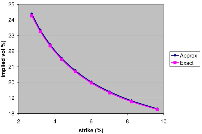
We consider a two-factor (2F) case of the Generalized multi-factor BK model (22),

r(t) =R(t) +e

S(t) (x1+x2)₋₁

S(t) , (24)

with the underlying processes

dxi(t) = (φi(t)−ai(t)xi(t))dt+γi(t)dWi(t), for i= 1,2,

starting from zero,xi(0) = 0, with a certain correlation between Brownian motions,

ρ(t) =E[dW1(t)dW2(t)].

We use standard data, summarized in the table below.

Rate R(t) 5.00%

Correlation ρ(t) -90.00%

Shift S(t) 10

Volatility 1 γ1(t) 1.00%

Volatility 2 γ2(t) 1.75%

Reversion 1 a1(t) 50.00%

Reversion 2 a2(t) 5.00%

18 19 20 21 22 23 24 25

2 4 6 8 10

strike (%)

implied

vol

%)

Approx Exact

Figure 1: Comparison of the implied vols for 10Y10Y European swaption (Generalized 2F BK model).

Exer (Y) Length (Y) Strike (%) Implied vol (%) Error (bps)

Approx Exact

5 10 3.28 25.77 25.71 5

5 10 3.67 25.04 24.99 6

5 10 4.10 24.34 24.31 3

5 10 4.59 23.69 23.67 2

5 10 5.13 23.09 23.09 0

5 10 5.73 22.53 22.54 -1

5 10 6.41 22.01 22.01 0

5 10 7.17 21.52 21.50 2

5 10 8.02 21.10 21.06 4

10 10 2.72 24.39 24.26 13

10 10 3.19 23.36 23.27 9

10 10 3.74 22.42 22.34 8

10 10 4.38 21.54 21.47 7

10 10 5.13 20.75 20.67 8

10 10 6.01 20.03 19.96 7

10 10 7.03 19.39 19.32 7

10 10 8.24 18.82 18.75 6

10 10 9.65 18.30 18.25 5

20 10 2.10 21.59 21.24 35

20 10 2.62 20.20 19.89 31

20 10 3.28 18.94 18.68 26

20 10 4.10 17.87 17.62 26

20 10 5.13 16.91 16.68 23

20 10 6.41 16.05 15.86 19

20 10 8.02 15.35 15.15 20

20 10 10.03 14.72 14.57 15

20 10 12.54 14.19 14.09 11

5.2

Bounded short rate model

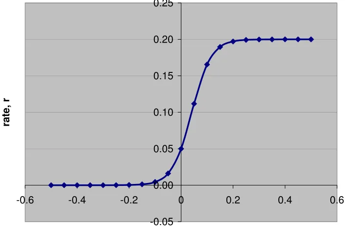
We consider a one-factor (1F) case of the Bounded short rate model (23),

r(t) =f(t, x) =U(t)e

β(t)x_+L(t)α(t)

eβ(t)x_+α(t) , (25)

with the underlying process

dx(t) = (φ(t)−a(t)x(t))dt+γ(t)dW(t),

starting from zero,x(0) = 0.

We use standard data, summarized in the table below.

Rate R(t) 5.00%

Volatility γ(t) 1.5%

Reversion a(t) 5.00%

Lower bound L(t) 0%

We have chosen particular time-independent parameters for transparency, however, the proposed ap-proximation works for general time-independent ones.

Below, we present a graphical visualization of the short rate dependence on the underlying variable.

-0.05 0.00 0.05 0.10 0.15 0.20 0.25

-0.6 -0.4 -0.2 0 0.2 0.4 0.6

underlying, x

ra

te

,

r

Figure 2: Rate as function of underlying,

r

=

f

(

x

).

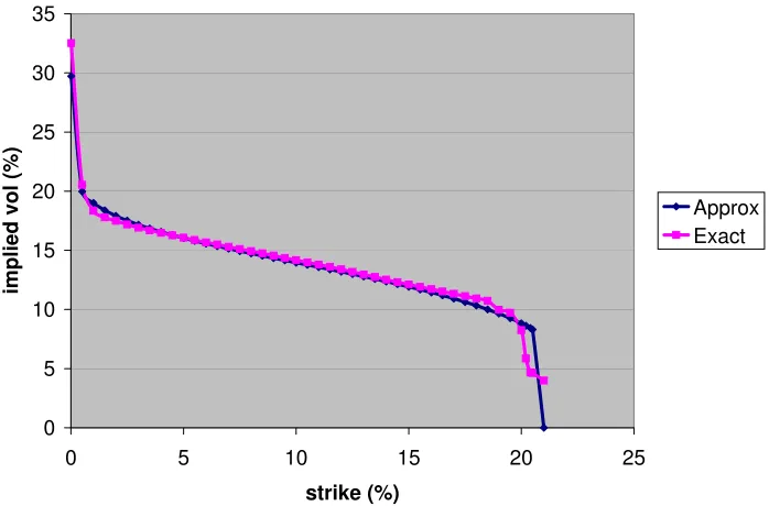
Strike (%) Implied vol (%) Error (bps)

Approx Exact

0.01 29.72 32.52 -280

0.5 19.98 20.54 -56

1 19.01 18.34 67

1.5 18.39 17.79 60

2 17.92 17.49 43

2.5 17.52 17.19 33

3 17.17 16.92 25

3.5 16.85 16.69 16

4 16.56 16.48 8

4.5 16.29 16.27 2

5 16.04 16.07 -3

5.5 15.8 15.87 -7

6 15.57 15.67 -10

6.5 15.35 15.49 -14

7 15.14 15.3 -16

7.5 14.93 15.11 -18

8 14.74 14.93 -19

8.5 14.54 14.74 -20

9 14.34 14.55 -21

9.5 14.15 14.36 -21

10 13.96 14.17 -21

10.5 13.77 13.98 -21

11 13.58 13.79 -21

11.5 13.38 13.6 -22

12 13.19 13.39 -20

12.5 12.99 13.18 -19

13 12.79 12.96 -17

13.5 12.58 12.74 -16

14 12.37 12.52 -15

14.5 12.14 12.31 -17

15 11.92 12.11 -19

15.5 11.69 11.91 -22

16 11.44 11.72 -28

16.5 11.19 11.52 -33

17 10.92 11.32 -40

17.5 10.63 11.12 -49

18 10.33 10.93 -60

18.5 10.01 10.73 -72

19 9.654 9.972 -31.8

19.5 9.263 9.724 -46.1

20 8.824 8.254 57

20.2 8.632 5.852 278

20.4 8.425 4.662 376.3

20.5 8.315 4.63 368.5

0 5 10 15 20 25 30 35

0 5 10 15 20 25

strike (%)

im

p

li

e

d

v

o

l

(%

)

Approx Exact

Figure 3: Comparison of the implied vols for 10Y10Y European swaption (Bounded short rate model).

6

Conclusion

In this article, we have treated generalized short rate models with Gaussian underlying (GSRG) and derived an efficient swaption price approximation. The result is based on a regular and singular expansion with respect to the small volatility and contains a low-dimensional integration.

We also presented two special cases of the GSRG model. The first one is the Generalized multi-factor Black-Karasinski (BK) model widely used by practitioners. The second one, Bounded short rate model, is new. Its rates evolve inside arbitrary thresholds. This model is especially attractive for scenario generation. The implied volatility skew for the Bounded short rate model is convex for small/moderate strikes and concave for bigger ones.

We have confirmed the analytical approximation quality by comparison with purely numerical results. We have detected an excellent analytics-numerics fit for short/medium maturities, and a good one for large maturities. We have observed a slight quality degeneration for extreme strikes.

The authors are indebted to Serguei Mechkov for discussions and numerical implementation help as well as to their colleagues at Numerix, especially to Gregory Whitten and Serguei Issakov for supporting this work and Patti Harris for the excellent editing. AA is grateful to Vladimir Piterbarg and Michael Konikov for stimulating discussions.

References

[1] F. Black and P. Karasinski (1991). Bond and Option pricing when Short rates are Lognormal, Fi-nancial Analysts Journal,47, 52-59.

[3] J. Hull and A. White (1990). Pricing interest-rate derivative securities, The Review of Financial Studies,3(4), 573–592.

[4] J. Hull and A. White (1994). Numerical procedures for implementing term structure models II: Two-factor models,Journal of Derivatives,2, 37–47.

[5] F. Tourrucˆoo, P. Hagan and G. Schleiniger (2007). Approximate Formulas for Zero-coupon Bonds,

Applied Mathematical Finance,14(3), 207–226.

[6] V. Piterbarg (2008). Practical Multi-Factor Quadratic Gaussian Models of Interest Rates, ICBI’s Global Derivatives Conference (Paris).

A

Zero-coupon bond

The parabolic operator underlying the zero-coupon bond PDE (8) reads

L(t, u) =−r(t, u) +εX

i

θi(t)∂i+ε

1 2

X

i,j

Cij(t)∂i∂j.

Denote an unperturbed operator asL0(t) and a perturbation asL1(t),

L0(t) = −r(t, u),

L1(t) = ε

X

i

θi(t)∂i+ε

1 2

X

i,j

Cij(t)∂i∂j.

A solution of the unperturbed equation

(∂t+L0(t))P0(t, T, u) = 0

for the unit final valueP0(T, T, u) = 1, will have a simple form,

P0(t, T, u) = exp −

Z T

t

dτ r(τ, u)

!

.

Using an unperturbed evolution operator,

U0(t1, t2) =:e Rt2

t₁ dτ L0(τ)

:=e−Rtt₁2dτ r(τ,u)

,

the bond priceP0(t, T, u) can be presented as a result of the action of the evolution operator on 1,

P0(t, T, u) =U0(t, T) 1.

The Dyson perturbation technique permits computing the first correction to the unperturbed solution

P1(t, T, u) =

Z T

t

dsLˆ1(t, s)P0(t, T, u), (26)

where ˆL1(t, s) is the dressed perturbation operator

ˆ

L1(t, s) =U0(t, s)L1(s)U

−1

0 (t, s). (27)

Rewrite the first correction in a more convenient way,

P1(t, T, u) =

Z T

t

ds U0(t, s)L1(s)U0(s, T) 1 =

Z T

t

ds P0(t, s, u)L1(s)P0(s, T, u). (28)

Differentiating the leading term, we obtain

L1(s)P0(s, T, u) =ε



 X

i

θi(s)∂i+

1 2

X

i,j

Cij(s)∂i∂j



P0(s, T, u) =εΛ(s, T, u)P0(s, T, u) (29)

for the multiplier

Λ(s, T, u) =−X

i

θi(s)gi(s, T, u) +

1 2

X

i,j

with

gi(s, T, u) =∂i

Z T

s

dτ r(τ, u) =

Z T

s

dτ ∂ir(τ, u)

and

gij(s, T, u) =∂i∂j

Z T

s

dτ r(τ, u) =

Z T

s

dτ ∂i∂ir(τ, u).

Finally, the first correction of the bond price reads

P1(t, T, u) =

Z T

t

ds P0(t, s, u)L1(s)P0(s, T, u)

= ε P0(t, T, u)

× Z T t ds    −X i

θi(s)gi(s, T, u) +

1 2

X

i,j

Cij(s)(gi(s, T, u)gj(s, T, u)−gij(s, T, u))







.

For completeness, we calculate the second order correction to the bond,

P2(t, T, u) =

Z T

t

ds1

Z T

s1

ds2Lˆ1(t, s1) ˆL1(t, s2)P0(t, T, u) (31)

= Z T t ds1 Z T s1

ds2P0(t, s1, u)L1(s1)P0(s1, s2, u)L1(s2)P0(s2, T, u). (32)

Using theL1 action on the leading order bond (29), we obtain

P2(t, T, u) =

Z T

t

ds1

Z T

s1

ds2P0(t, s1, u)L1(s1) (Λ(s2, T, u)P0(s1, T, u)).

Calculating the action of theL1on the product in the r.h.s.,

L1(s1) (Λ(s2, T, u)P0(s1, T, u)) = P0(s1, T, u)L1(s1) (Λ(s2, T, u)) + Λ(s2, T, u)L1(s1) (P0(s1, T, u))

+ X

i,j

Cij(s1)∂jΛ(s2, T, u)∂iP0(s1, T, u),

we can further simplify the second correction to the bond price

P2(t, T, u) = P0(t, T, u)

   1 2 Z T t

dsΛ(s, T, u)

!2 + Z T t ds1 Z T s1 ds2 

L1(s1) Λ(s2, T, u)−

X

i,j

Cij(s1)gi(s1, T, u)∂jΛ(s2, T, u)

     (33) or

P2(t, T, u) = P0(t, T, u)

   1 2 Z T t

dsΛ(s, T, u)

!2 + Z T t ds1 X i 

θi(s1)−

X

j

Cij(s1)gj(s1, T, u)



 Z T

s1

ds2∂iΛ(s2, T, u)

+ 1 2 Z T t ds1 X ij

Cij(s1)

Z T

s1

ds2∂i∂jΛ(s2, T, u)







where the derivatives of the multiplier are

∂iΛ(s, T, u) = −

X

k

θk(s)gik(s, T, u) +

1 2

X

kn

Ckn(s) (2gki(s, T, u)gn(s, T, u)−gnki(s, T, u)))

∂i∂jΛ(s, T, u) = −

X

k

θk(s)gijk(s, T, u)

+ 1

2

X

kn

Ckn(s) (2gkij(s, T, u)gn(s, T, u) + 2gki(s, T, u)gjn(s, T, u)−gnkij(s, T, u)))

andgijkn(s, T, u) =∂i∂j∂k∂ng(s, T, u), as usual.

B

AD price

In the case of the AD price, we deal with asingular perturbation technique. The AD price satisfies the forward PDE (∂t−L∗(t, u) )q(t, u) = 0 with the parabolic operator

L∗

(t, u) =−r(t, u)−εX

i

θi(t)∂i+

1 2ε

X

i,j

Cij(t)∂i∂j

and the initial conditionq(0, u) =Q

iδ(ui−yi(0)).

It is easy to check that the Gaussian density

q0(t, u) =

exp −1 2ε

−1_{(u−ε m(t))}T_V−1_{(t)(u−ε m(t))}

(2π ε)n2 |V(t)| 1 2

,

where m(t) is they(t) center andV(t) is the covariance in vector/matrix notations, satisfies the PDE

∂tq0(t, u) =−ε

X

i

θi(t)∂iq0(t, u) +1

2ε

X

i,j

Cij(t)∂i∂jq0(t, u).

The Gaussian density derivatives look as follows,

∂tq0(t, u)

q0(t, u) =

1 2ε

−1_{(u−ε m(t))}T_V−1_(t)C(t)V−1_{(t) (u−ε m(t)) +θ}T_(t)V−1_{(t) (u−ε m(t))}

− 1

2trC(t)V

−1_(t),

∂iq0(t, u)

q0(t, u)

= −ε−1 _V−1_{(t) (u−ε m(t))}

i,

∂i∂jq0(t, u)

q0(t, u)

= ε−2

V−1_{(t) (u−ε m(t))}

i V

−1_{(t) (u−ε m(t))}

j−ε

−1

V−1_(t)

ij,

where we have used the relations

∂tV

−1_{(t) = −V}−1_(t)∂

tV(t)V

−1_{(t) =−V}−1_(t)C(t)V−1_(t),

∂tln|V(t)| = tr∂tV(t)V

−1_{(t) = trC(t)}

V−1_(t).

Now, following the Heat-Kernel expansion logic, we look for the solution as

where Ω(t, u) is aregular function ofεwith the unit initial condition Ω(0, u) = 1. After substitution into the initial PDE, we get an equation on the Ω(t, u),

∂tΩ(t, u) = −r(t, u) Ω(t, u)−ε

X

i

θi(t)∂iΩ(t, u)

+ 1

2ε

X

i,j

Cij(t)∂i∂jΩ(t, u) +ε

X

i,j

Cij(t)∂ilnq0(t, u)∂iΩ(t, u).

Or, using the derivative of the Gaussian∂ilnq0(t, u), we obtain

∂tΩ(t, u) +r(t, u) Ω(t, u) +uTV

−1_{(t)C(t)∂Ω(t, u)}

+ ε

θT(t)∂Ω(t, u)−1

2tr C(t)∂

2_{Ω(t, u)−m}T_(t)V−1_{(t)C(t)∂Ω(t, u)}

= 0, (35)

where we have used vector notations for the first derivatives ∂ = {∂1, ∂2,· · · } and the drifts θ = {θ1, θ2,· · · }, and matrix notations for the second derivatives (∂2)ij =∂i∂j.

We will look for the solution Ω as a regular expansion inε,

Ω(t, u) =b0(t, u) +ε b1(t, u) +· · · (36)

with the initial conditionsb0(t, u) = 1 and b1(t, u) = 0.

The leading-order solution will satisfy the unperturbed PDE

∂tb0(t, u) +uTV−1(t)C(t)∂ b0(t, u) +r(t, u)b0(t, u) = 0. (37)

This is a linear first-order PDE with characteristics (passing throughuat time τ)

uc(t, τ, u) =V(τ)V

−1_(t)u,

which can be derived from the fact that

∂t+uTV−1(t)C(t)∂ V−1(t)u= 0. Thus, the solution has

the following form,

b0(t, u) = exp

−

Z t

0

ds r s, V(s)V−1_(t)

u

. (38)

The derivatives in matrix notations read

∂tb0(t, u)

b0(t, u)

= −r(t, u) +uT V−1_(t)C(t)V−1_(t)h(1)_{(t, u),}

∂b0(t, u)

b0(t, u)

= −V−1_(t)h(1)_{(t, u),}

∂2b0(t, u)

b0(t, u)

= V−1_(t)h

h(1)(t, u)⊗h(1)(t, u)−h(2)(t, u)iV−1_(t),

where we denoted the vector

h(1)_n (t, u) =X

j

Z t

0

ds Vnk(s) ˜∂kr s, V(s)V−1(t)u (39)

and the matrix

h(2)_nl(t, u) =X

km

Z t

0

ds Vnk(s) ˜∂k∂˜mr s, V(s)V

−1_(t)

Here, the derivative ˜∂kdenotes the short rate derivative over the space argument, ˜∂ir(s, z(u)) = ∂r_∂z(s,zi(u(u))).

Proceed now to the first correction,b1(t, u). After substituting the expansion (36) into the PDE (35)

and retaining the first-order terms inε, we obtain

∂tb1(t, u) +uTV

−1_(t)C(t)

∂ b1(t, u) +r(t, u)b1(t, u) =g(t, u), (41)

where the r.h.s. reads

g(t, u) = −θT(t)∂ b0(t, u) +

1

2tr C(t)∂

2

b0(t, u) +mT(t)V

−1_(t)C(t)

∂ b0(t, u)

= b0(t, u)

n

θT(t)−mT(t)V−1_(t)C(t)

V−1_(t)h(1)_{(t, u)}

+ 1

2 tr C(t)V

−1_(t)h

h(1)(t, u)⊗h(1)(t, u)−h(2)(t, u)iV−1_(t)

.

It is easy to see that the first correction has the following solution,

b1(t, u) =e

−Rt

0ds r(s,V(s)V− 1

(t)u) Z t

0

dτ g(τ, V(τ)V−1_(t)u)eRτ

0 ds r(s,V(s)V− 1

(t)u)_{. (42)}

After some algebra, we arrive at

b1(t, u) = b0(t, u)

×

Z t

0

dτ θT(τ)−mT(τ)V−1_(τ)C(τ)

V−1_{(τ) ˆh}(1)_{(τ;t, u)}

+ 1

2

Z t

0

dτ tr V−1_(τ)C(τ)V−1_(τ)h_hˆ(1)_{(τ;t, u)⊗hˆ}(1)_{(τ;t, u)−hˆ}(2)_{(τ;t, u)}i

,

where

ˆ

h(1)_n (τ;t, u) = X

j

Z τ

0

ds Vnk(s) ˜∂kr s, V(s)V−1(t)u,

ˆ

h(2)_nl(τ;t, u) = X

km

Z τ

0

ds Vnk(s) ˜∂k∂˜mr s, V(s)V

−1_(t)u

Vml(s).

Finally, the AD price, up to the first order in small volatilities, looks as follows,

q(t, u) = exp −

1 2ε

−1_{(u−ε m(t))}T_V−1_{(t)(u−ε m(t))}

(2π ε)n2 |V(t)| 1 2 exp − Z t 0

ds r s, V(s)V−1_(t)

u

×

1 +ε

Z t

0

dτ θT(τ)−mT(τ)V−1_(τ)C(τ)

V−1_{(τ) ˆ}

h(1)(τ;t, u)

+ 1

2ε

Z t

0

dτ tr V−1_(τ)C(τ)V−1_(τ)h_ˆh(1)_{(τ;t, u)⊗ˆh}(1)_{(τ;t, u)−ˆh}(2)_{(τ;t, u)}i