Low Power and Simple Implementation of Secure Hashing Algorithm (SHA-2) using VHDL Implemented on FPGA of SHA-224/256 Core

(1)

73 Copyright © 2018. IJEMR. All Rights Reserved.

Volume-8, Issue-1 February 2018

International Journal of Engineering and Management Research

Page Number: 73-78

Synthesis of Redundant Planar Isotropic Manipulator using Link Length

Ratios

Hareesha N G1 and K N Umesh2

1_{Assistant Professor, Department of Aeronautical Engineering, Dayananda Sagar College of Engineering, Bengaluru,} Karnataka, INDIA

2 _{Professor, Department of Mechanical Engineering, PES College of Engineering, Mandya, Karnataka, INDIA}

1

Corresponding Author: [email protected]

ABSTRACT

This research involves synthesis of planar isotropic 3R manipulator using link length ratios. A novel method is proposed to obtain exact solutions for synthesis of the manipulator using the conditions of isotropy. Two earlier methods of synthesis are used to compare the proposed method and are shown to be more appropriate and precise enough to get eight isotropic configurations.

Keywords— Planar manipulator, Kinematic Synthesis, Isotropy, Redundant Manipulator, Condition Number

I. INTRODUCTION

Isotropic configurations are considered as the best configurations within the workspace of any manipulator [1] for the following reasons – (i) best servo accuracy can be achieved, (ii) likelihood of error is minimal and equal in all directions and (iii) velocity and force transmission is uniform at these isotropic configurations for the norm input. The optimal kinematic synthesis of robotic linkages is an important task in the field of robotics. While designing such linkages, one should consider the isotropic configurations of the linkages.

Many research works are focused on kinematic isotropy since last 30 years. Condition number of a Jacobian of manipulator [1], Manipulability ellipsoid [2], Global isotropy index [3] are the few measures available on kinematic isotropy. The present work uses condition number and manipulability ellipsoid as measure of isotropy. The condition number of a Jacobian is unity and manipulability ellipsoid becomes a circle for isotropic manipulator. The condition number “one” indicates that there is no scaling of error. At isotropic configuration, manipulability ellipse becomes circle. Circle indicates that

velocity distribution at the tip of the manipulator is uniform. Kinematic isotropy has been applied to planar 2 DOF [4], 3DOF [4]–[6] and 4 DOF and above [4], [5], [7] for mechanism design. Fully isotropic parallel manipulators are also designed [8]. Kinematic isotropy has been applied for optimum design of parallel manipulators [6], [9]. Isotropy of redundant manipulator is challenging compared to non-redundant manipulators since its Jacobian is not a square matrix. Finding inverse of such rectangular matrix is tedious. Nevertheless, many researchers have synthesized redundant manipulators [10]– [13] using kinematic isotropy. Most related methods are taken here for comparison with proposed method. ManJa Kircanski [4] has developed a method to find all isotropic configurations of planar 2R and 3R manipulator.

The equations are developed for maximum and minimum singular values and condition number is expressed as a function of second Joint angle, θ2, and ratio of link lengths l1 and l2 ( i.e., k=l1/l2). In the case of 3R manipulator, two link length ratios, k1 = l1/l3 and k2 = l2/l3 are taken for synthesis. It has been shown that, there are eight isotropic configurations for planar 3R manipulator. Given the link length ratios k1 and k2, isotropic configurations are determined. K.Y. Tsai [5] has developed another method to find the isotropic configurations of planar 3R manipulators. Two equations are obtained, in terms of second and third Joint displacements, using the conditions of kinematic isotropy.

(2)

74 Copyright © 2018. IJEMR. All Rights Reserved.

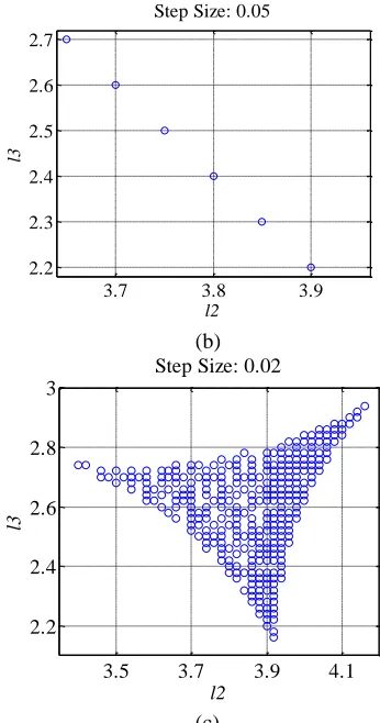
isotropic configurations) can‟t be obtained. A step size of 0.1 yields, three sets of link lengths (i.e., 3.7, 3.7, 2.6; 3.8, 3.8, 2.4; 3.9, 3.9, 2.2) as shown in Figure 1 (a). Similarly, step size of 0.05 yields six sets as shown in Figure 1(b) and step size of 0.02 gives more sets as shown in Figure 1(c). Number of sets of link lengths is dependent on step size and constraints used. As the step size reduces, time taken to search the set of link lengths increases. Hence, there is a need for an alternate and quick method for solving the problem.

II. SYNTHESIS OF ISOTROPIC

MANIPULATORS

A 2R manipulator is considered for obtaining the link length ratio for isotropy. Using the properties of 2R manipulator, isotropic configurations of 3R manipulators are obtained.

A. Conditions for Isotropic Manipulators

For non-redundant manipulators such as 2R manipulator as shown in Figure 2, Jacobian „J‟ of manipulator is a square matrix. When the manipulator is in isotropic configuration, Jacobian of the manipulator becomes orthogonal and satisfies the condition:

[I] [J][J] [J]

[J]T  T (1)

where [I] is an identity matrix.

But, for redundant manipulators, condition defined in (1) is not valid, since J is a rectangular matrix. In such case, [J]T[J][J][J]T. The condition[J]T[J][I], means that the columns of J are orthogonal. This can only happen if J is an m×n matrix with n < m. Similarly

[I]

[J][J]T means that the rows of J are orthogonal, which requires n > m. Where „m‟ is the number of rows

and „n‟ is the number of columns of the Jacobian. „m‟

defines the task space and „n‟ defines number of Joints in

the manipulator.

Step size: 0.1

3.7 3.8 3.9

2.2 2.4 2.6

l2

l3

Step Size: 0.1

(a)

3.7 3.8 3.9

2.2 2.3 2.4 2.5 2.6 2.7

l2

l3

Step Size: 0.05

(b)

3.5 3.7 3.9 4.1

2.2 2.4 2.6 2.8 3

l2

l3

Step Size: 0.02

(c)

Figure 1. Sets of link length which give eight solutions

The conditions for isotropy of 2R manipulators may be defined as:

For orthogonality of rows of J, 0 

 T

2 1 2 T

1J J J J

For equality of the magnitude of columns of J, ||J1|| = ||J2||

(2a)

(2b)

where J1 and J2 are the rows of the Jacobian J.

Isotropic conditions for redundant manipulators are slightly different from non-redundant manipulators. For orthogonality of rows of J,

0



T 2 1J

J

For equality of the magnitude of columns of J, ||J1|| = ||J2||.

(3a)

(3b)

Using the conditions defined in (3), system of equations can be obtained.

B. Isotropy of Planar 2R manipulator

(3)

75 Copyright © 2018. IJEMR. All Rights Reserved.

O2

q

1 l1 l2 x y

q

2 End effector

Figure 2. Planar 2R manipulator in general configuration

The Jacobian of the manipulator is,

           12 2 12 2 1 1 12 2 12 2 1 1 c l c l c l s l s l s l

J J1 J2 (4)

where l1, l2 are the link lengths andθ1,θ2 are the absolute

Joint angles. s₁sinq₁ ; s₂sinq₂; c1cosq1; c2cosq2. UsingJ₁TJ₂0;

0 )

(

)

(

)

(

)

(



l

₁

s

₁



Using ||J1|| = ||J2|| ;



 



2

12 2 2 12 2 2 12 2 1 1 2 12 2 1

1s l s lc l c l s l c

l      

 (6)

Solving (5) and (6) simultaneously, we get, 2 2 1 _ l l (7)

It can be noticed here that taking the ratio of link lengths, i.e., l1/l2 = 2, isotropic configurations of 2R manipulator can be obtained. Using this property of link length ratios, we prove that the isotropic configurations of 3R manipulators can be easily determined.

C. Isotropy of Planar 3R manipulator

Consider a planar 3R manipulator as shown in Figure 3. O1 O2 O3 q1 l1 l2 l3 x y End effector q3 q2

Figure 3. Planar 3R manipulator in general configuration

Jacobian of the manipulator „J‟ with respect to tip of the manipulator is given in (8).

                3 3 3 3 2 2 3 3 2 2 1 1 3 3 3 3 2 2 3 3 2 2 1 1 c l c l c l c l c l c l s l s l s l s l s l s l

J (8)

              2 1 23 22 21 13 12 11 J J J J J J J J

where l1, l2, l3 are the link lengths andq1, q2 and q3are

corresponding absolute Joint angles. J1 and J2 are row vectors of J; s₃sinq₃; and c₃cosq₃.

Using the conditions defined in (3), it can be written as,

 T 2 1J J 0 2 2 3

2₂2 ₂ ₂ ₃2 ₃ ₃ ₂₃ ₂ ₃ ₂₃ ₃ ₂

3 3 1 2 2

1      

ll s ll s l c s l c s l l c s l l c s

(9) ||J1|| = ||J2|| =

3 3 1 2 2 1 2 1 2 3 2 3 2 2 2 2 2 3 2 3 2 2 2

2 3 2 3 2 2

2l s  l c  l c  l s l  ll c  ll c

0 4

42323 2323

 l lcc llss (10)

Equations (9) and (10) are two simultaneous non-linear equations consisting of three link lengths and four trigonometric functions. These unknowns should be determined in order to get the isotropic configurations of planar 3R manipulator. Since it is not possible to solve these two equations with seven unknowns, trigonometric identities are used to eliminate two variables from (9) and (10). Using, 2 2 1 2 x x s   and 2 2 2 1 1 x x c  

 (11)

2 3 1 2 y y s 

 and ₂

2 3 1 1 y y c  

 (12)

where,        2 tan q2

x and _

      2 tan q3

y (13)

Substituting for s2, s3, c2and c3 from (11) and (12) into (9) and (10), and simplifying, it can be written, that

(4)

76 Copyright © 2018. IJEMR. All Rights Reserved.

0

1 2 1 2

1 2 3 2 4

1 2 1 2

1 2 3 2 4

     

 _

    

 _

    

 _

     

 _

    

 _

    

 _



y x

x y l l

y x

y x l l

(15)

Equations (14) and (15) are two highly non-linear simultaneous equations with five unknown variables, namely, l1, l2, l3, x and y. It is not possible to solve equations (14) and (15), unless we eliminate some variables or use some constraints. K.Y. Tsai [5] has used exhaustive search method to find link lengths l1, l2, l3 which satisfy the equations (14) and (15). But, in the proposed method, keeping the link lengths ratio equal to 2, isotropic configurations are obtained. Using,

2

3 2 3 1 _ _

l l l l

(16)

Equation (16) will be satisfied if

l

₁



l

₂



2

and

l

3



1

.

Thus, using these link lengths in (14) and (15),

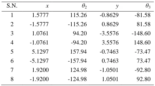
The equation (21) is solved using fsolve function of Maple and verified using solve function of MATLAB. Both yield the same results. The results obtained are tabulated in the Table 1. Real roots of the polynomial are tabulated in Table 1 (column-2). Substituting each value of y into equation (13), θ3 is obtained. Substituting the real roots of the quartic polynomial in to (17) and (18), two 4th degree polynomials with only one variable (x) are obtained. When solved, each polynomial will give either two or four real roots. Out of these, any two roots will satisfy both (17) and (18) along with corresponding value of y. Using any one out of two, second Joint displacements (θ2) are computed using equation (13) and results are tabulated in column-3. The results used for calculation of

θ2 are given in column-2.

D. Isotropic configurations

Joint displacements obtained as discussed in previous section are absolute Joint angles in degrees. These absolute Joint angles are converted into relative Joint angles and are plotted as shown in Figure 4.

It is noticed that, Joint angles given in Table 1 are not much different from the results obtained by T Sai [5]. Singular values are different since link lengths ( 2, 2, 1) are different compared to link lengths (3.7, 3.7, 2.6) used. An important observation is, if link lengths are multiplied by any common scalar (c), same Joint angles can be obtained. Hence, there is no limitation in terms of link lengths which give isotropic configurations.

Table 1: Real roots and corresponding absolute Joint angles

S.N. x θ2 y θ3

1 1.5777 115.26 -0.8629 -81.58

2 -1.5777 -115.26 0.8629 81.58

3 1.0761 94.20 -3.5576 -148.60

4 -1.0761 -94.20 3.5576 148.60

5 5.1297 157.94 -0.7463 -73.47

6 -5.1297 -157.94 0.7463 73.47

7 1.9200 124.98 -1.0501 -92.80

8 -1.9200 -124.98 1.0501 92.80

E. Advantages and limitations

The main advantages and limitations of the method are enumerated here.

Advantages:

i) Scaling factors can be used for link lengths depending upon requirement. There is no need to search for link lengths using constraints and searching algorithm. The method is completely analytical and no numerical search is required for searching link lengths. This reduces the time of computation and ensures host of unique solutions.

ii) Since the system of equations is substituted with link length, it becomes very convenient while computing the solutions.

iii) The method is faster and more accurate as the approach is completely analytical.

Limitations:

(g)

q

₂= 125o,

q

₃= -92.8o (h)

q

₂= -125o,

q

₃= 92.8o

Figure 4: Isotropic configurations with absolute Joint angles

REFERENCES

[1] J. K. Salisbury & J. J. Craig. (1982). Articulated hands: Force control and kinematic issues. The International

Journal of Robotics Research, 1(1), 4–17.

[2] Y. YokokohJi, J. S. Martin, & M. FuJiwara. (2009). Dynamic manipulability of multifingered grasping. IEEE Transactions on Robotics, 25(4), 947–954.

[3] F. Stocco, Leo J, salcudean, Septimiu E, & Sassani. (1997). Mechanism design for global isotropy with applications to haptic interfaces. The Winter Annual Meeting of the ASME Sixth Annual Symposium on Haptic Interfaces for Virtual Environment and Teleoperator Systems, 1–8.

[4] M. Kirćanski. (1996). Kinematic isotropy and optimal kinematic design of planar manipulators and a 3-DOF spatial manipulator. International Journal of Robotics Research, 15(1), 61–77.

[5] K. Y. Tsai, P. Y. Lin, & T. K. Lee. (2008). 4R spatial and 5R parallel manipulators that can reach maximum number of isotropic positions. Mechanism and Machine Theory, 43(1), 68–79.

[6] X. J. Liu, Z. L. Jin, & F. Gao. (2000). Optimum design of 3-DOF spherical parallel manipulators with respect to the conditioning and stiffness indices. Mechanism and Machine Theory, 35, 1257–1267.

[7] C.-H. Dai, & Jian Sheng, Kuo (2011). A fully-isotropic parallel orientation mechanism. 13th World Congress in Mechanism and Machine Science, GuanaJuato, México, 1– 7.

[8] G. Gogu. (2004). Fully-isotropic over-constrained planar parallel manipulators. International Conference on lntelligenl Robots and Systems, 3519–3524.

[9] H. S. Kim & L.-W. Tsai. (2003). Design optimization of a cartesian parallel manipulator. Journal of Mechanical Design, 125(1), 43-51.

[10] I. Ebrahimi, J. A. Carretero, & R. Boudreau. (2008). Kinematic analysis and path planning of a new kinematically redundant planar parallel manipulator.

Robotica, 26(3), 405–413.

[11] K. Y. Tsai & Z. W. Wang. (2005). The design of redundant isotropic manipulators with special link parameters. Robotica, 23(2), 231–237.

[12] K. N. Umesh & C. Amarnath. (2015). Motion properties of planar two-degree-of-freedom mechanisms.

Mechanism and Machine Theory, 38(4), 345–354.