Http://www.ijetmr.com©International Journal of Engineering Technologies and Management Research [15]
ANALYSIS OF SURFACE ROUGHNESS MILLED OF STEEL AISI 1045
USING X-BAR AND R CONTROL CHART
Leonardo Geraldo Leite 1, Ítalo de Abreu Gonçalves 1, Carlos Henrique de Oliveira 1,
Tarcísio Gonçalves de Brito 1, Sandra Miranda Neves 1, Emerson José de Paiva 1 1 Federal University of Itajubá, Itabira, MG, Brazil
Abstract:
The steel milling AISI 1045 has been gaining prominence in industry in recent years as it allows machined parts to be obtained with low-cost inserts. However, to ensure the final product quality, it is important that the milling for machining procedure be well planned in order to the cutters have their wear minimized in the process, as well as a considerable productivity rate with a zero occurrence of reworked parts or scraps. Thus, this paper presents a study about the quality of the machined surface on the end milling process of AISI 1045 steel using titanium nitride (TiN) coated carbide inserts, optimized for a combined design, using Design of Experiments (DOE). Statistical Process Control (SPC) is applied to analyze the process variations using X-bar and R control charts. The objective of this study is to identify the optimal combination of the input setup such as cutting speed (Vc), feed per tooth (fZ), work penetration (ae) and machining depth (ap) that is capable of minimize the process variation. The response measured is the roughness parameter Ra, observed under the influence of cutting fluid, tool wear, concentration and flow of the cutting fluid as noise. The obtained result was the stability of the Ra roughness for the AISI 1045 steel in end milling process, which is not influenced by noise variables due to Robust Parameter Design used in this study.
Keywords: End Milling; Control Chart; Roughness; Design of Experiments.
Cite This Article: Leonardo Geraldo Leite, Ítalo de Abreu Gonçalves, Carlos Henrique de Oliveira, Tarcísio Gonçalves de Brito, Sandra Miranda Neves, and Emerson José de Paiva. (2018). “ANALYSIS OF SURFACE ROUGHNESS MILLED OF STEEL AISI 1045 USING X-BAR AND R CONTROL CHART.” International Journal of Engineering Technologies and Management Research, 5(6), 15-23. DOI: https://doi.org/10.29121/ijetmr.v5.i6.2018.242.
1. Introduction
Http://www.ijetmr.com©International Journal of Engineering Technologies and Management Research [16] One of these variables is the use of cutting fluids in milling operations that can bring several advantages to the process, which is the reason for the growing interest among researchers in the field. According to Brito (2015), the use of cutting fluids in milling processes is aimed at the cooling of the tool and work piece produced for high cutting speeds, better surface finishing and smoothing the wear, which is a natural phenomenon of the process. In order to ensure a consistent and robust quality, the development of products should be low sensitive to fluctuations inherent to the manufacturing process that may change its variability. The use of cutting fluids, for example, when analyzed from the perspective of concentration and flow, can cause variations in the manufacturing process, leading to unexpected results and reducing the robustness of the system.
According to Taguchi (1986), a reasonable way to optimize a robust process is to summarize the data of a cross-matrix experiment with the mean of each observation in the internal matrix through all the executions in the external matrix, being combined in the signal-to-noise ratio. Welch et al. (1990) proposed the replacement of the cross-arrangement by the combined arrangement, both with controllable and noise factors, applying this approach to computational experiments, through simulation. This same approach was applied by Shoemaker et al. (1991) in experiments in physics. The Robust Parameter Design (RPD) approach, with a combined array, treats both controllable and noise variables in the same way, using a model capable of assess all the parameters main effects and interactions, including interactions between control and noise variables (MONTGOMERY, 2013, BRITO et al 2014).
The use of techniques to plan experiments in order to generate data that result in objective and valid conclusions is the main objective of statistics. The planning of the experiments, called Design of Experiments (DOE), advocates the simultaneous variation of the factors involved in an experiment with the objective of constructing prediction models for the responses of interest. Each different combination of factor levels gives the name of treatment for the analyzed set (MONTGOMERY, 2013). According to Grine et al. (2010) and Haridy et al. (2010), the Design of Experiments (DOE) is a structured and organized method to determine the relationship between the different input and output factors of the process, involving the definition of the set of experiments, in which all relevant factors are systematically varied.
The variability between the different inputs and outputs factors of the process presents possible causes that make it unstable and unreliable. According to Caruso and Helleno (2009), the use of Statistical Process Control(SPC) will involve the use of Control Charts, to determine their characteristics when the production processes undergo changes and how much these changes can affect the product quality (FERREIRA; MEDEIROS; OLIVEIRA, 2007). For Paladini (2002), the SPC has tools that allow a detailed analysis of the productive process to develop actions to improve the process, being a set of concepts and tools that bases the quality management.
Http://www.ijetmr.com©International Journal of Engineering Technologies and Management Research [17] (LCL) on each side of the centerline of the process, this tool presents accurate results and, when well interpreted, leads to a better process understanding, predictability and reliability.
The aim of this paper is to analyze the stability of surface roughness (Ra) ofend milling of AISI
1045 steel found in the work of Brito (2015), by using a Taguchi L9 and X-bar and R Control Charts for the confirmation runs. The Taguchi design allowed the assessment for the robustness of optimal setup, formed by cutting speed (vc), feed rate per tooth (fz), work penetration (ae),
machining depth (ap) under different noise combinationsof noise variables like tool wear (vb),
Cutting fluid concentration (C) and Cutting fluid flow rate (Q).
2. Control Charts
Control Charts stand out as the main element of Statistical Process Control (SPC), a graphical representation that, given the history of data presented, allows the identification of certain behaviors of the process over time and also the detection of special causes. According to Linna& Woodall (2001), Control Charts are tools used to monitor the accuracy of a production process over time by verifying observed deviations from known patterns.
The development of Control Charts requires the plotting of representative points from the measurements made and the addition of three lines, one central and the other control ones. Control lines, also referred to as Lower Control Limit (LCL) and Upper Control Limit (UCL), are calculated from a dispersion measure and have the objective of alerting if the process has suffered some disturbance that may interfere with its state of statistical control (ALMAS, 2003).
According to Montgomery (2016), for the determination of the upper and lower control limits of control charts, for 𝑋̅ and R, the Eq. (1-4) are used:
Mean:
n X
LSC
2
d R 3 +
= (1)
n X
LIC
2
d R 3 −
= (2)
693 . 1
2 =
d
Amplitude:
2 3
d R 3d R
LSC = + (3)
2 3
d R 3d R
LIC = − (4)
888 . 0
3 =
Http://www.ijetmr.com©International Journal of Engineering Technologies and Management Research [18] Ramos (2003) suggests that the procedure of constructing control graphs involves, in general, sampling of fixed sizes at sample intervals. Through these samples, we obtain estimates for the mean level, dispersion and specific limits of the process. In order to build a Control Chart, samples of fixed size n must be extracted from the process to be analyzed, which may or may not have the same periodicity, which usually depends on the availability of samples, collection difficulty or even cost. For Montgomery (2005), it is recommended that 20 to 25 samples be taken to test whether the process is stable and within the required parameters. For processes in which a particular cause is identified in the preparation of this first assessment, the point should be discarded and its control limits recalculated based only on the remaining points. The points should then be reexamined, repeating this process until all points are under control (MONTGOMERY, 2005).
In order for the process represented in the graph to be considered stable, or under control, the points plotted on the graph must be within the stipulated limits. The presence of one or more points outside the control limits, or non-randomly dispersed, represents instability of the graph and, consequently, in the process. The presence of points within the limits of control, however, does not provide enough information to identify the stability of the process, which for Pozzobon (2001), requires a more detailed analysis of the points from eight situations that portray the probability of process is out of statistical control, such as:
• One or more points beyond the control limits;
• Nine successive points on the same side of the central value, either above or below the mean;
• Six successive points increasing or decreasing constantly; • Fourteen successive points alternating up and down;
• Two of three successive points in the same zone or beyond;
• Four in five successive points, located at the ends of the control limits, on the same side of the graph;
• Fifteen successive points in the zone below or above the center line; • Eight successive points on both sides of the centerline.
3. Experimental Procedure
The analyzed experiments were obtained from Brito (2015) on end milling in AISI 1045 steel, using response surface methodology in a combined arrangement, built in MINITAB software, for analysis. A Central Composite Design (CCD) was created for seven variables, four of which were control variables: feedrate per tooth (fz), machining depth (ap), cut speed (vc) and work penetration
(ae), and three independent variables (noise): tool wear (vb), Cutting fluid concentration (C) and
Http://www.ijetmr.com©International Journal of Engineering Technologies and Management Research [19] Table 1: Control variables and their levels.
Milling parameters Unit Notation Levels
-2.828 -1 0 1 2.828
Feed rate per tooth mm/tooth fz 0.01 0.10 0.15 0.20 0.29
Machining depth mm ap 0.064 0.750 1.125 1.500 2.186
Cuts peed m/min vc 254 300 325 350 396
Work Penetration mm ae 12.26 15.00 16.50 18.00 20.74
Table 2: Noise variables and their levels.
Noises Unit Notation Levels
-1 0 1
Tool flank wear mm vb 0.00 0.15 0.30
Cutting fluid concentration % C 5 10 15
Cutting fluid flow rate l/min Q 0 10 20
In the carried out experiment, a CNC machining center by brand Fadal was used, with 15 kW of power and maximum rotation of 7,500 rpm. The material used in the milling process was the AISI-1045 steel with dimensions 100 x 100 x 300 mm and an average hardness of 180 HB. The tool used was aend milling cutter code R390-025A25-11M, diameter 25 mm, position angle Xr = 90 °, cylindrical rod, medium pitch with 3 carbide inserts ISSO P25, code R390-11T308M-PM GC 1025 (Sandvik-Coromant) coated with titanium nitride (TiN) and mechanical clamping. The cutting fluid applied during the machining process was Quimatic MEII synthetic oil.
A stereoscopic microscopic Magnification model with magnification of 45x and digital camera coupled for acquisition of images was used to measure the wear of the tool. For the end of the tool life, the criterion of flank wear of vbmax = 0.30 mm was adopted. The mean Raroughness, recorded
by a Mitutoyo Surftest 201 portable rugosimeter, measured in three points of the work piece, one at the center and the other at each end, in order to consider the mean value of the readings.
After determining the optimal point according to the results showed on Brito (2015), a Taguchi L9 design was created to evaluate the optimized configuration behavior in a nine different scenarios formed by noise variables. The optimal control variables setup used by Brito (2015) were defined by using optimized weights of 0.80 and 0.20, whereas for this study, it was also used an optimal point regarding the weights of 0.95 and 0.05, with control variables setup defined asfz = 0.15
mm/tooth, ap = 1.22 mm, vc = 391.59 m/min , ae = 16.5 mm. Table (3) presents the confirmation
experiments in nine different conditions for Tool wear (vb), Cutting fluid concentration (C) and
Cutting fluid flow rate (Q).
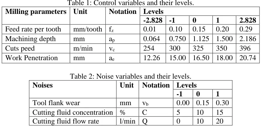
Table 3: Results of confirmation experiments.
Tool wear (vb)
(mm)
Cutting fluid concentration (C) (%)
Cutting fluid flow rate (Q) (l/min)
Measurements Ra1 Ra2 Ra3 Meanof
Ra
0 5 0 1 0.56 0.57 0.58 0.57
Http://www.ijetmr.com©International Journal of Engineering Technologies and Management Research [20]
0 5 0 3 0.57 0.58 0.55 0.57
0 10 10 1 0.58 0.53 0.54 0.55
0 10 10 2 0.57 0.58 0.58 0.58
0 10 10 3 0.58 0.57 0.59 0.58
0 15 20 1 0.58 0.55 0.59 0.57
0 15 20 2 0.54 0.57 0.55 0.55
0 15 20 3 0.6 0.58 0.57 0.58
0.15 5 10 1 0.58 0.6 0.54 0.57
0.15 5 10 2 0.52 0.57 0.53 0.54
0.15 5 10 3 0.56 0.53 0.57 0.55
0.15 10 20 1 0.59 0.55 0.54 0.56
0.15 10 20 2 0.57 0.53 0.56 0.55
0.15 10 20 3 0.55 0.59 0.57 0.57
0.15 15 0 1 0.54 0.58 0.55 0.56
0.15 15 0 2 0.55 0.54 0.59 0.56
0.15 15 0 3 0.53 0.56 0.55 0.55
0.3 5 20 1 0.59 0.57 0.54 0.57
0.3 5 20 2 0.53 0.52 0.55 0.53
0.3 5 20 3 0.57 0.58 0.56 0.57
0.3 10 0 1 0.56 0.53 0.55 0.55
0.3 10 0 2 0.53 0.54 0.58 0.55
0.3 10 0 3 0.57 0.56 0.55 0.56
0.3 15 10 1 0.57 0.55 0.53 0.55
0.3 15 10 2 0.56 0.58 0.57 0.57
0.3 15 10 3 0.59 0.54 0.55 0.56
4. Results and Discussions
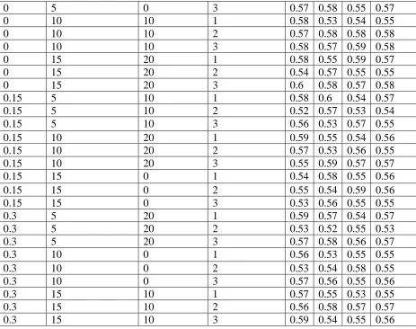
Figure (1) shows the roughness Ra behavior, for mean and amplitude, for optimized samples of 27
experiments. The values do not present variation, since they do not extrapolate the control limits defined in the graph. For Pozzobon (2001), the simple observation of the presence of points outside the control limits does not provide sufficient conclusions about the stability of the process, and it is necessary to analyze the graph from eight situations in which there is a probability that the process is outside of control.
Http://www.ijetmr.com©International Journal of Engineering Technologies and Management Research [21] Figure 1: X-bar & R control chart for Roughness Ra
Figure (2) shows the roughness Ra behavior for 3 types of tools: new tools, worn at 0.15 mm and
worn at 0.30 mm, according to Taguchi's L9 arrangement, resulting in differences between the stages. In relation to the finishing of the milled surface, made with tool worn with 0.15mm vbmax,
presented a small variation for mean and amplitude in relation to the new and worn tools in 0.30mm, with its more wide control limits. The cause may be related to the fact that the cutting tool presents irregular surface, more accentuated due to its natural wear. From the point of view of the milling process, the new tools leave grooves more defined by the edges, presenting bigger roughnesses even in the finishes. As they wear out by use, the tools increase the radius of the contact edge with the work piece, which leads to better finishes because the contact surface (radius of tip) is less pronounced, generating shallow grooves and less prominent and, consequently, minor roughness. From the process control standards, it is possible to verify that the roughness remained stable for values of the mean and amplitude, despite the small variations in the responses as a function of tool wear.
Figure 2: Roughness Ra controlgraph regarding tool wear (vb)
25 22 19 16 13 10 7
4 1 0,60
0,58
0,56
0,54
0,52
Sample
Sa
m
pl
e
M
ea
n
__ X=0,56012 UCL=0,59726
LCL=0,52299
25 22 19 16 13 10 7
4 1 0,08 0,06 0,04 0,02 0,00
Sample
Sa
m
pl
e
Ra
ng
e
_ R=0,0363 UCL=0,0934
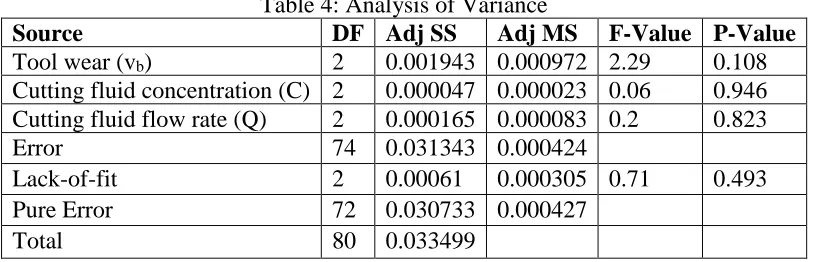
Http://www.ijetmr.com©International Journal of Engineering Technologies and Management Research [22] With Taguchi´s L9 arrangement verified by Analysis of Variance (ANOVA), tab. (4) presents the results of this analysis with P-Value above the level of 5% of significance for all noise variables, ie, all analyzed noise factors do not significantly influence Ra responses, which proves the stability
of the system, justifying the identification of the Robust Parameter Project for this condition.
Table 4: Analysis of Variance
Source DF Adj SS Adj MS F-Value P-Value
Tool wear (vb) 2 0.001943 0.000972 2.29 0.108
Cutting fluid concentration (C) 2 0.000047 0.000023 0.06 0.946 Cutting fluid flow rate (Q) 2 0.000165 0.000083 0.2 0.823
Error 74 0.031343 0.000424
Lack-of-fit 2 0.00061 0.000305 0.71 0.493
Pure Error 72 0.030733 0.000427
Total 80 0.033499
The non-influence of noise variables can be reaffirmed by Lack-of-Fit, a regression test that exhibits lack of fit when it does not adequately describe the relation between experimental factors and response variables, which for this paper lists the noise variables with Roughness Ra. The
P-Value for Lack-of-Fit is higher than the level of expected significance, which indicates the stability condition of the system. The stability of the system proves that the noise variables, the main sources of instabilities for any manufacturing process, did not influence the response variable analyzed. Analysis of variance (ANOVA) showed that tool wear, concentration and flow rate of the cutting fluid had no influence on the surface roughness of the milled parts.
5. Conclusion
After the confirmation experiments and Ra roughness measurements, it was possible to establish
the Control Chart for AISI 1045 steel milling. The results show that the process behaved in a stable manner, which allows us to state that it is under control, based on the eight criteria required to validate a statistical chart. This stability is due to the contribution of the Robust Parameter Design that proves that the noise variables, the main sources of instability for any manufacturing project, did not influence in the response of the variable analyzed. The behavior of the RaRoughness was
not influenced by any noise variable tested.
Acknowledgements
The authors would like to thank Capes, CNPQ and Fapemig for their support on this research and the resources dispensed to realize this work.
References
[1] ALMAS, Fabio. Implementation of Statistical Process Control in a textile company. Masters dissertation. Itajubá(MG): UNIFEI, 2003.
Http://www.ijetmr.com©International Journal of Engineering Technologies and Management Research [23]
[3] BRITO, T. G.; PAIVA, A. P. ; GOMES, J. H. F. ; BALESTRASSI, P. P. . A normal boundary intersection approach to multi response robust optimization of the surface roughness in end milling process with combined arrays. Precision Engineering, v. 38, p. 628-638, 2014.
[4] CARUSO, D. M; HELLENO, A. L. Six Sigma: a conceptual approach with management methodology or tool for quality improvement. In: XXIXNational Meeting of Production Engineering Production Engineering and Sustainable Development: Integrating Technology and Management. Anais. Salvador, BA,Brasil, 06 to 09 ofoctoberof 2009.
[5] De MAGALHAES, M.S; MOURA NETO, F.D. Economic-statistical design of variable parametersnon-central chi-square control chart. Production Journal, 21, pp. 259-270. 2011. [6] DINIZ, A. E., MARCONDES, F. C., COPPINI, N. L. Material machining technology. 6ª ed. São
Paulo: Artliber Publisher, p. 262, 2014.
[7] FERREIRA, P. O; MEDEIROS, P. G; OLIVEIRA, L. M. Use of statistical process control for monitoring the mean weight of tuberculostatic capsules: a case study. In: XXVIII National Meeting of Production Engineering. The integration of productive chains with the sustainable manufacturing approach. Anais. Rio de Janeiro, RJ, Brasil, 13 to 16 ofoctober de 2008.
[8] GRINE, K., ATTAR, A., AOUBED, A., BREYSSE, D. (2010) Using the design of experiment to model the effect of silica sand and cement on crushing properties of carbonate sand. Materials and Structures, v. 44, pp. 195-203.
[9] HARIDY, S., GOUDA, S. A., WU, Z. (2010). An integrated framework of statistical process control and design of experiments for optimizing wire electrochemical turning process. International Journal of Advanced Manufacturing Technology, DOI 10.1007/s00170-010- 2828-7. [10] LINNA, K. W., WOODALL, W. H., Effect of Measurement Error on Shewhart Control Chart,
Journal of Quality Technology, vol. 33, nº 2, April 2001.
[11] MONTGOMERY, D. C. Design and Analysis of Experiments. 6ª ed. Nova York: John Wiley & Sons, p. 643, 2005.
[12] MONTGOMERY, D. C. Introduction to statistical quality control. 7ª ed. Rio de Janeiro: LTC, 2016.
[13] MONTGOMERY, Douglas C.. Introduction to statistical quality control. Rio de Janeiro: LTC, 2013.
[14] PALADINI, Edson Pacheco. StrategicQuality Assessment. São Paulo: Atlas, 2002. POZZOBON, E. M. P. Application of Statistical Process Control. Master's Dissertation - Post-Graduation Program in Production Engineering. Federal University of Santa Maria, Santa Maria, 2001.
[15] RAMOS, E. M. L. S., Improvement and Development of Tools of Statistical Quality Control - Using Quartiles to Estimate Standard Deviation, Doctoral Thesis by the Federal University of Santa Catarina, Florianópolis, April 2003.
[16] SANDVIK COROMANT. Technical Machining Manual, Sandviken, Suécia, 2011.
[17] SHOEMAKER, A. C.; TSUI, K. L.; WU, C. F. J. Economical experimentation methods for robust design. Technometrics, v. 33, n. 4, 1991.
[18] SNEDECOR, G.W. & Cochran, W.G. (1980), Statistical Methods. 7th ed., The Iowa State Univ. Press, Iowa, USA.
[19] TAGUCHI, G. Introduction to Quality Engineering: Designing Quality into Products and Process. Tokyo, Japan: Asian Productivity Organization, 1986.
[20] WELCH, W. J., YU, T. K., KANG, S. M., SACKS, J. Computer Experiments for Quality Control by Parameter Design, Journal of Quality Technology, v. 22, p. 15-22, 1990.
*Corresponding author.