Internetworking Indonesia Journal

(1)

signal for eye focuses which consists of three eyes movement left, top, and right. The electroencephalography (EEG) data were recorded from eight volunteers including males and females. The volunteers were stimulated using designed steady-state visual evoked potential (SSVEP) to gaze the designed SSVEP. The acquired EEG data were processed using wavelet decomposition and reconstruction. The reconstructed and decomposed signals were used as features to the input of artificial neural network (ANN). Based on the classification results, the decomposed signals of D1 give the best performance with the average accuracy of 98 % for validation, 67.19 % for validation, and 60.94 % for testing.

Index Terms—Classification; EEG; Artificial neural networks (ANN); Steady-state visual evoked potential (SSVEP); Wavelet.

I. INTRODUCTION

UMAN body has electrical conductivity properties which are able to distribute electrical signal and even evoke the electrical signal. Brain is human’s organ that formed by neurons which can produce a potential electrical energy known as neuro-electrical potential. Electroencephalography (EEG) is an electrophysiological monitoring method that measures brain’s neural activities. The EEG signal describes brain’s state which has a relation with human’s mental condition. The EEG signal is commonly represented by low-voltage signal versus time graph [1]. Some stimuli produce EEG signal and special features called even-related potential (ERP). ERP is a special potential evoked by brain activities, which deliberately stimulate and create psychological differences significantly [2].

One of common EEG stimulus methods is steady-state visual evoked potential (SSVEP). SSVEP is oscillation of EEG signal evoked in the visual cortex when someone focuses on periodically flickered stimulus [3]. To produce a SSVEP response, a visual stimulus must be presented to the subject. SSVEP represents focus level on rapidly flickered stimulus. It is dominant at occipital region. In the brain computer interface (BCI) SSVEP test, subjects were asked to focus on various flickered item. When subject concentrates, SSVEP activities at

Manuscript received October 22, 2016.

W. Caesarendra , M. Ariyanto, and K. A. Pambudi are with the Mechanical Engineering Department, Diponegoro University, Jl. Prof. Sudarto, SH – Tembalang, Semarang 50275, Indonesia (e-mail: [email protected];[email protected];

[email protected] )

Syahara U. Lekson was with the Mechanical Engineering Department,Diponegoro University, Jl. Prof. Sudarto, SH – Tembalang, Semarang50275, Indonesia (e-mail: [email protected] ).

certain frequency can be identified. BCI SSVEP is the fastest BCI but also needs a little training. In the other hand, SSVEP is easily distracted by subjects fatigue when they focus on the flickered item [4].

Support vector machine (SVM) [5-6] and artificial neural network (ANN) [7-8] are widely used as classifier in EEG signal analysis because these methods provide great performance in classification of EEG signal. In this paper, the decomposed EEG signal from wavelet transform is used prior to the ANN classification. The network outputs are the eye focus in left, top, or right. The EEG signal input is stimulated using our designed SSVEP. The decomposed EEG signals of D1, D2, and D3 from wavelet transform are used to study the best features for the classification results.

II.MATERIALS

A.Subjects

The EEG data were acquired from eight subjects as shown in Table I. The age is between 21 and 31 years old. The subject eye conditions are 4 subjects with healthy eye and 4 subjects with myopia. There are two subjects that do not have prior knowledge about the EEG system i.e. Subject 7 and 8.

TABLEI SUBJECTS DESCRIPTION

Subject Sex Age Eye condition

1 Male 22 Normal

2 Male 21 Myopia (-4.0)

4 Male 25 Normal

5 Female 22 Myopia (-4.0)

7 Male 31 Normal

8 Male 28 Normal

B.Devices

The experiment used MITSAR-EEG-202 with international pattern 10-20. It has 32 channel recorder for data acquisition and 1388 x 720 pixels monitor to display the visual stimulus. It is suitable for the recording, observation and spectral analysis of the EEG, video EEG monitoring and evoked potentials recording.

C.Softwares

The EEG data were acquired using WinEEG software from Mitsar. WinEEG allows for the recording, editing and

Classification of EEG Signals for Eye Focuses

Using Artificial Neural Network

Wahyu Caesarendra, Mochammad Ariyanto, Kharisma A. Pambudi, M. Faizal Amri, Arjon Turnip

(2)

analysis of continuously recorded EEG. The EEGlab interactive MATLAB toolbox was selected to convert data type from WinEEG to MATLAB readable data type. For the data processing, feature extraction, and classification of EEG signal were conducted in MATLAB environment.

III. METHODS

A.Wavelet Transform

A wavelet is a waveform of effectively limited duration that has an average value of zero and nonzero norm [5]. Sine wave and wavelets have differences in the length of signal and amplitude with respect to the time. Sine wave range from minus to plus infinity or do not has limited duration. Sine wave is smooth and predictable while wavelet is irregular and asymmetric. The sine wave and wavelet picture are depicted in Figure.1.

Figure.1 Sine wave signal compared to wavelet [5]

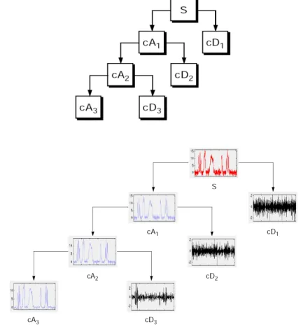
The wavelet decomposition process can be iterated, with successive approximations being decomposed. As shown in Fig. 2, the wavelet decomposition vector c from wavelet decomposition tree can be shown in Figure.2(a), while the picture of signal decomposition can be shown in Figure.2(b). Figure.2 shows that one signal can be broken down into many lower-resolution components.

Figure.2 Wavelet decomposition: (a) Wavelet decomposition chart up to 3 level decomposition, where cA and cD is low frequency part and high frequency part, respectively; (b) Signal decomposition illustration using wavelet [5]

Extending wavelet reconstruction technique to the components of a multi-level analysis, it is found that similar relationships hold for all the reconstructed signal constituents

[5]. There are several ways to reassemble the original signal in wavelet reconstruction. One of them is shown in Figure.3 and can be expressed in (1).

Figure.3 Schematic of reconstructed signal [5]

1 1

2 2 1

3 3 2 1

S

A

D

S

A

D

S

A

D

=

+

=

+

=

+

(1)

B.Artificial Neural Network (ANN)

The experiment used MITSAR-EEG-202 with international pattern 10-20. It has 32 channel recorder for data acquisition and 1388 x 720 pixels monitor to display the visual stimulus. It is suitable for the recording, observation and spectral analysis of the EEG, video EEG monitoring and evoked potentials recording.

Artificial neural network (ANN) is a computation system in which the architecture and the operation are based on neurological science. ANN is model that emulates how biological neural works. Basically, there are two types of ANN architecture; single layer of neurons and multi-layer of neurons [6]. In one layer of neuron, each element of input vector p is connected with neuron input through weight matrix

W. An i numbers of neuron collects weighted input and bias b. The neuron of i is processed by function activation or transfer function of layer f. The neuron layers output f is output vector

a. The illustrated figure of one layer of neuron is shown in Figure.4.

The output of neuron (a) in layer can be defined as in (2)

1 1,1 1 1

(

)

a

=

f W

p

+

b

(2)

(3)

In multi-layer of neurons, the ANN structure comprises of more than one layer. Each layer has weight matrix W, input vector p, a bias vector b, and an output vector a. In each layer has function activation or transfer function of layer f. Layer on the multi-layer network has different process. A layer which is next to the input is called hidden layer and a layer that is next to the output of network is called output layer. The structure of multi-layer of neurons is presented in Figure.5.

The output of neuron (a) in the first layer can be defined as expressed in (3)

1 1,1 1 1

( )

a = f IW p +b (3) The output of neuron (a) in the second layer is defined as in (4)

2 2 2,1 1 1,1 1 1 2

(

)

a

=

f

LW

f

IW

p

+

b

+

b

(4)

Finally, the output of neuron (a) in the third layer can be described as in (5)

2 3 3,1 2 2,1 1 1,1 1 1 2 3

(

)

a

=

f

LW

f

LW

f

IW

p

+

b

+

b

+

b

(5)

Figure.5 Multi-layer of neurons [6]

In this study, the multi-layer of neural network which comprises of one hidden layer and one output layer is employed. The input of the neural network is the processed EEG signal obtained from wavelet decomposition process. The network ouputs are left, top, or right of eye focus. The network used 20 neurons in hidden layer. The other selected neural network parameters and its description is summarized in Table II.

TABLEII SET-UP PARAMETERS OF ANN Parameter Descripton

Model Feed forward neural

network

Number of neuron 20

Devide parameter Random

Ratio of training 70%

Ratio of validation 15%

Ratio of testing 15%

Training algoritm Levenberg-Marquardt backpropagation

Maximum epoch 100

Performance goal 0.001

Minimum gradient 1x10-7

Error performance Mean squared normalized error

Transfer function of

layer 1 Radial basis function

Transfer function of

layer 2 Saturating linear function

IV. STEADY-STATE VISUAL EVOKED POTENTIAL

To produce a SSVEP response from EEG, a visual stimulus must be given to the subject. Each subject has to complete two offline experimental sessions. The distance between monitor and eye was 30 cm for the first session and 40 cm for the second session. Each session consists of 28 stimuli. The subjects were asked to focus and follow the gaze on the target shown in monitor. The duration of each session is 5 minutes.

The order of stimulus appearance is from left, above, and right and then appears again from left with different shape of stimulus. The sequence of shape is rectangular, circle, and triangle as shown in Figure.6. Color of the stimulus changes after right triangle stimulus. The order of color is red, yellow, and blue. The utilized monitor is 16 : 9 with pixels dimension 1366 x 768. The rectangular, circle, and triangle of stimuli have r value to define its dimension. The defined dimension of each shape is defined by Figure.7. The selected value of r is 4 pixels. Each stimulus runs for 3 seconds and flickers at 6 Hz. Time interval between stimulation is 2 seconds.

Figure.6 Sequence images of stimulus on the monitor

(4)

There were 7 channels used during experiment that are O1, O2, Pz, Fz, Cz, P3, and P4. All EEG signals data were saved from each subject using WinEEG software. The size of EEG data of each subject was 7 x 1 arrays. The placement of the utilized electrodes on the head of each subject can be seen in Figure.8.

Figure.8 EEG electrodes application diagram [7]

V. RESULTS AND DISCUSSION

Prior to processing step, the EEG signal are normalized to zero mean. The first processing step employed short time Fourier transform (STFT) method. The processed result of STFT is shown in Figure.9. Figure.9 shows that there is very low amplitude in the range of 40-60 Hz. It is because the EEG amplifier has a hardware notch filter that allows suppressing the power line noise at 50 Hz. Based on the STFT results, the next process is to filter the EEG signal using low pass filter with cut-off frequency at 40 Hz. The processed frequency of EEG signal above 40 Hz is not used in this classification method. The original signal and filtered signal using low pass filter is shown in Figure.10.

Figure.9 STFT of EEG signal

Figure.10 (a) Raw signal; (b) Filtered signal

The second processing step employed wavelet decomposition method. Each subject produced seven EEG signals. The decomposition of EEG signal utilizes “haar” method. The decomposed EEG signal is divided into three subset; D1, D2, and D3. The subset is employed to the input of neural network classifier. Figure.11 shows the result of decomposed EEG signal that will be used as features. The first row of Figure.11 represents the original signal (S). The second, third, and fourth row of Figure.11 indicate the decomposed signal of D1, D2, and D3, respectively.

Figure.11 Wavelet decomposition result

The result of decomposition method is a matrix 7 x 54 for each subject. Where 7 indicates seven channels of EEG data and 54 columns means 54 times of acquisition in gaze direction. Each subject has 18 data gaze direction in the left, 18 data in the top, and 18 data in the right.

Frequency-domain feature extraction based on fast Fourier transform (FFT) are used in this study. The features used are the average amplitude of each frequency band. The frequency is divided into five subsets, theta for 4-8 Hz, alpha for 8-13 Hz, beta low for 13-23 Hz, beta high for 23-30 Hz, and gammafor 30-40 Hz. The final input features size is 35 rows for each subject (7 channels x 5 frequency bands). The final input data became matrix with the size of 35 x 54.

The ANN classifier is developed in MATLAB environment. The selected parameters of ANN classifier is summarized in Table III that is presented before. The input for each subject is 35 x 54 matrixes and the output of the neural network is 3 x 1. Three rows mean the classification results left, top, or right. The decomposed EEG signals of D1, D2, and D3 are used in this study to calculate the best result of decomposed signals. Levenberg-Marquardt back propagation training algorithm is used for better classification results.

The classification of EEG signal stimulated by SSVEP is summarized in Table III, Table IV and, Table V. Each table shows the classification results using decomposed EEG signal for D1, D2, and D3, respectively.

(a)

(5)

ANN CONFUSION MATRIX RESULTS FOR D1

Subject Accuracy (%)

Training Validation Testing All

1 97.4 62.5 62.5 87.0

2 100.0 50.0 37.5 83.3

3 97.4 62.5 37.5 83.3

4 94.7 50.0 50.0 81.5

5 100.0 50.0 50.0 85.2

6 100.0 75.0 100.0 96.3

7 100.0 50.0 50.0 85.2

8 97.4 50.0 37.5 81.5

Average 98.36 56.25 53.12 85.41

TABLEIV

1 94.7 75 62.5 87

2 100 50 50 85.2

3 97.4 50 25 79.6

4 100 37.5 75 87

5 92.1 75 50 83.3

6 100 100 100 100

7 100 62.5 75 90.7

8 100 87.5 50 90.7

Average 98 67.19 60.94 87.94

TABLEV

1 94.7 50 75 85.2

2 86.8 50 25 72

3 97.4 37.5 37.5 79.6

4 92.1 25 50 75.9

5 100 37.5 37.5 81.5

6 100 100 100 100

7 100 50 37.5 83.3

8 100 62.5 25 83.3

Average 96.38 51.56 48.44 82.6

Based on the classification results on the Table III to V, it can be summarized that the average training results of all subjects are 98.36% for D1, 98% for D2 and 96.38% for D3. For the confusion result during validation, the averages of all subjects are 56.25 % for D1, 67.19% for D2 and 51.56 % for D3. Average testing results of all subjects are 53.12% for D1, 60.94 % for D2 and 48.44 % for D3. The accuracy of testing is not high enough. These results show that quantity of data for training is not enough. The classification accuracy of ANN

will increase as the number of data for training is larger. For the overall classification results, the average results of all subjects are 85.41% for D1, 87.94 % for D2 and 82.6% for D3.

VI. CONCLUSION

Based on the results, it can be concluded that the decomposed EEG signal D2 gives the best results. There is no relationship between the subject who knows about EEG and subject who does not know about EEG. Top three classification results are subjects 6, 1, 5 and the lowest three classification results are subject 2,3,4. Subject 7 and 8 are in the middle rank. To improve the classification results, the artifact on the EEG signal needs to be processed with advanced preprocessing technique.

In the future research, the EEG electrodes placed near the temples, or to the sides of the eyes, would be able to get higher accuracy classification results as eye.

ACKNOWLEDGMENT

Authors thank to Dr. Arjon Turnip from Indonesian

Institute of Sciences for the EEG data.

REFERENCES

[1] T. Radüntz, J. Scouten, O. Hochmuth, B. Meffert, EEG artifact elimination by extraction of ICA-component features using image processing algorithms, Journal of Neuroscience Methods, Volume 243, 30 March 2015, pp. 84-93.

[2] Y. Wu, S. Huang, H. Xiao, “The Application of EEG related”, Procedia Environmental Sciences, Volume 10, 2011, pp. 1338-1342.

[3] M. Oqaibi, M. Ali Fattouh. “An Enhanced SSVEP BCI Application Through Emotion: Preliminary Results”. International Journal of Innovative Research in Computer and Communication Engineering.

2015, pp. 12080-12089.

[4] M. Wang, I. Daly, B. Z. Allison, J. Jin, Y. Zhang, L. Chen, X. Wang, A new hybrid BCI paradigm based on P300 and SSVEP, Journal of Neuroscience Methods, Volume 244, 15 April 2015, pp. 16-25. [5] H.L. Jian and K.T. Tang, "Improving classification accuracy of SSVEP

based BCI using RBF SVM with signal quality evaluation," Intelligent Signal Processing and Communication Systems (ISPACS), 2014 International Symposium on, Kuching, 2014, pp. 302-306.

[6] O. Dehzangi, Y. Zou and R. Jafari, "Simultaneous classification of motor imagery and SSVEP EEG signals," Neural Engineering (NER), 2013 6th International IEEE/EMBS Conference on, San Diego, CA, 2013, pp. 1303-1306.

[7] H. Cecotti and A. Graeser, "Convolutional Neural Network with embedded Fourier Transform for EEG classification," Pattern Recognition, 2008. ICPR 2008. 19th International Conference on, Tampa, FL, 2008, pp. 1-4.

[8] W. Caesarendra, M. Ariyanto, S. U. Lexon, E. D. Pasmanasari, C. R. Chang and J. D. Setiawan, "EEG based pattern recognition method for classification of different mental tasking: Preliminary study for stroke survivors in Indonesia," 2015 International Conference on Automation, Cognitive Science, Optics, Micro Electro-Mechanical System, and Information Technology (ICACOMIT), Bandung, 2015, pp. 138-144. [9] M. H. Beale, M. T. Hagan, and H. B. Demuth. Wavelet Toolbox:

User’s Guide MATLAB. MathWorks. 1996.

[10] M. H. Beale, M. T. Hagan, dan H. B. Demuth. Neural Network Toolbox: User’s Guide MATLAB. MathWork. 2015.

(6)

Wahyu Caesarendra received B.Sc. degree from Department of Mechanical Engineering, Diponegoro University, Indonesia in 2010, and M. Eng. from Pukyong National University Korea. He got PhD degree in University of Wollongong Australia in 2015. Currently, he is a Lecturer at Diponegoro University, Semarang, Indonesia. His research interests are signal processing, pattern recognition, and mechatronics.

Mochammad Ariyanto received B.Sc. and M.Sc. degrees from

Department of Mechanical Engineering, Diponegoro University, Indonesia, in 2010 and 2013 respectively. Currently, he is a Lecturer at Diponegoro University, Semarang, Indonesia. His research interests are robotics, biomechatronics, and intelligent control.

Kharisma A. Pambudi is undergraduate student at Mechanical

Engineering Diponegoro University. Her researches include robotics and neural network.

Syahara U. Lekson received her B.Sc. degree in Mechanical Engineering