The Use of Wavelet Transformation in Conjunction with a Heuristic Algorithm as a Tool for Feature Extraction from Signals

(1)

Information Technology and Control 2017/3/46 372

ITC 3/46

Journal of Information Technology and Control

Vol. 46 / No. 3 / 2017 pp. 372-381

DOI 10.5755/j01.itc.46.3.17582 © Kaunas University of Technology

The Use of Wavelet Transformation in Conjunction with a Heuristic Algorithm as a Tool for Feature Extraction

from Signals

Received 2017/03/23 Accepted after revision 2017/07/03

http://dx.doi.org/10.5755/j01.itc.46.3.17582

The Use of Wavelet Transformation

in Conjunction with a Heuristic

Algorithm as a Tool for Feature

Extraction from Signals

Dawid Połap and Marcin Woźniak

Institute of Mathematics, Silesian University of Technology, Kaszubska 23, 44-100 Gliwice, Poland e-mail: [email protected], [email protected]

Corresponding author: [email protected]

The use of algorithms is helpful in analysis of various data samples. Examples of these applications are sound and graphic processing that are used in authentication and analysis of images. In this work, we propose tech-nique of extracting data from image file created based on voice sample. Proposed method makes use of math-ematical model of wavelet transformation and its graphical visualization like scaleogram combined with com-putational intelligence methods like neural network and heuristic algorithm. In order to verify operation of proposed technique we present experimental results.

KEYWORDS: Neural networks, speaker recognition, wavelet transformation, heuristic algorithm, feature extraction, image processing.

1. Introduction

Nowadays, audio signals are very common for their applications in many areas of today life. First of all, search for new forms of security and identity verifica-tion is necessary. Classical soluverifica-tions do not support fast and reliable verification, but cause queues of work-ers in large corporations. It is one of motivations to improve and seek alternative solutions. Of course, it is

(2)

373 Information Technology and Control 2017/3/46

for metal stamping. Signals find their use also in soft

computing like user identity verification in smart-phones [5, 12] and speaker recognition for micro ma-nipulation of robots [20]. It is highly recommended that all systems work automatically and that was pre-sented in [1]. The idea of automatic speech recognition was presented for under-resourced languages [14], which can data structures for knowledge storing [6, 7]. Application is among topics, which scientists are fo-cused on, but on the other hand, theoretical aspects of analysis and its functionality are very important. In [16], authors analyzed high resolution property of group delay function in terms of signals processing and for contrast of all theoretical aspects, in [8] wavelet decom-position for vibration simulation signal was shown. The use of signals requires many other tools like pro-cessing and classification methods. The most popular classifiers are grouped into two type - fuzzy and neu-ral. In the first type, fuzzy approach is based on rough set and in [11], authors presented method for fast im-age classification based on that idea. It may be hard to define a specific value in fuzzy controller, that is why some researches work on definition of less, more

etc. [15]. The second type is neural network which is simplified model of human brain. Some application of such solution is presented in [13] where authors showed the idea of classification using incomplete or missing data. All possible solutions are created based on processing methods [10] and modeling as well as some rules which are called programming languages [18, 4]. Mentioned rules are related to data record, which is required for certain embodiments of tech-nology. And in [14] number of advantages and disad-vantages of software-solution architectures were presented. Similarly, heuristics are currently used in various models to simulate and optimize [2, 17]. In this paper, we would like to connect few of these ideas linked in effective tool for feature extraction from voice signals. We presented selected application (like voice verification) as a tool for testing our ap-proach and an indication of its advantages.

2. Wavelet Transform

The history of wavelet theory dates back to early twen-tieth century, when Hungarian mathematician, Alfred Haar presented the first known wavelet (today known

as Haar wavelet) [9]. The author applied orthonormal wavelet to show an example of system in interval < 0,1 >. That wavelet is function defined as follows

�(�) � �

�� _� ��_��

. (1)

70 years later, French geophysicist, Jean Morlet has introduced formal definition of wavelet.

Definition 1. Wavelet is a function ψa,b :R→R coming from parent function ψ with scaling a and shift b (in effect giving entire family of functions). Wavelet of scale a and shift b is defined as follows

8

��,�(�) = �(2�� ). (2)

�(�) = 2sinc(2�) − sinc(�) =��(��)��(��)_�� , (3)

sinc(�) = �� (��)�� 0

� �� = 0. (4)

��,�(�) =_√�� _� �, (5) where ��_� � is called core of transformation, and � � 0.

�_��|�(�)|_� �� , (6)

� �(�)�� = 0_�� . (7)

�̂�(�, �) =_√�� (�)� �_�� _� ��. (8)

�(�) = � �_��|�(�)|_� ��

� ��

� � �̂�� (�, �)� ��_� �� (9)

�̂�(�, �) = � �_�� _�,�(�)�(�)��. (10)

��,�= �� _�_�� , �, � � �. (11)

��(�, �) = � �� ,�(�)�(�)��. (12)

�(�) = ��∑ ∑ �� (�, �)��,�(�), (12)

(2)

The creation of formal definition of wavelet allowed for rapid growth of mathematical aspects associated with it. Within few years, researchers have worked on models applicable for transformation and its funda-mental operations.

2.1 Continuous Wavelet Transform

In wavelet representation, signal is projected onto continuous family of frequencies. In most cases, band-width is scaled in scale equal to 1 and shifted by parent function. An example of such function is sinc(x), what can be presented as

8

��,�(�) = �(2�� ). (2)

�(�) = 2sinc(2�) − sinc(�) =��(��)��(��)_�� , (3)

sinc(�) = �� (��)�� 0

� �� = 0. (4)

�_��|�(�)|_� �� , (6)

� �(�)�� = 0_�� . (7)

�̂�(�, �) =_√�� (�)� �_�� _� ��. (8)

�(�) = �

�_��|�(�)|_� ��

� � �̂�(�, �)� � ��

� � �

�� (9)

�̂�(�, �) = � �_�� _�,�(�)�(�)��. (10)

��,�= �� _�_�� , �, � � �. (11)

��(�, �) = � �� ,�(�)�(�)��. (12)

�(�) = ��∑ ∑ �� (�, �)��,�(�), (12) (3)

where

8

��,�(�) = �(2�� ). (2)

�(�) = 2sinc(2�) − sinc(�) =��(��)��(��)_�� , (3)

sinc(�) = �� (��)�� 0

� �� = 0. (4)

�_��|�(�)|_� �� , (6)

� �(�)�� = 0_�� . (7)

�̂�(�, �) =_√�� (�)� �_�� _� ��. (8)

�(�) = �

�_��|�(�)|_� ��

� � �̂�(�, �)� � ��

� � �

�� (9)

�̂�(�, �) = � �_�� _�,�(�)�(�)��. (10)

��,�= �� _�_�� , �, � � �. (11)

��(�, �) = � �� ,�(�)�(�)��. (12)

�(�) = ��∑ ∑ �� (�, �)��,�(�), (12)

(4)

Generalizing, subspaces in scale a are generated by positively defined function (called child function) and presented as

8

��,�(�) = �(2�� ). (2)

�(�) = 2sinc(2�) − sinc(�) =��(��)��(��)_�� , (3)

sinc(�) = �� (��)�� 0

� �� = 0. (4)

��,�(�) =_√�� _� �, (5)

where ��_� � is called core of transformation, and � � 0.

�_��|�(�)|_� �� , (6)

� �(�)�� = 0_�� . (7)

�̂�(�, �) =_√�� (�)� �_�� _� ��. (8)

�(�) = �

�_��|�(�)|_� ��

�

� � �̂�(�, �)� � ��

� � �

�� (9)

�̂�(�, �) = � �� ,�(�)�(�)��. (10)

��,�= �� _�_�� , �, � � �. (11)

��(�, �) = � �_�� _�,�(�)�(�)��. (12)

�(�) = ��∑ ∑ �� (�, �)��,�(�), (12)

, (5)

where

8

��,�(�) = �(2�� ). (2)

�(�) = 2sinc(2�) − sinc(�) =��(��)��(��)_�� , (3)

sinc(�) = �� (��)�� 0

� �� = 0. (4)

��,�(�) =_√�� _� �, (5)

�_��|�(�)|_� �� , (6)

� �(�)�� = 0_�� . (7)

�̂�(�, �) =_√�� (�)� �_�� _� ��. (8)

�(�) = �

�_��|�(�)|_� ��

�

� � �̂�(�, �)� �

��

�� (9)

�̂�(�, �) = � �_�� _�,�(�)�(�)��. (10)

��,� = �� _�_�� , �, � � �. (11)

��(�, �) = � �_�� _�,�(�)�(�)��. (12)

�(�) = ��∑ ∑ �� (�, �)��,�(�), (12)

(3)

8

��,�(�) = �(2�� ). (2)

�(�) = 2sinc(2�) − sinc(�) =��(��)��(��)_�� , (3)

sinc(�) = �� (��)�� 0

� �� = 0. (4)

��,�(�) =_√�� _� �, (5)

�_��|�(�)|_� �� , (6)

� �(�)�� = 0_�� . (7)

�̂�(�, �) =_√�� (�)� �_�� _� ��. (8)

�(�) = � �_��|�(�)|_� �� ̂�(�, �)� � ��

�� (9)

�̂�(�, �) = � �_�� _�,�(�)�(�)��. (10)

��,�= �� _�_�� , �, � � �. (11)

��(�, �) = � �_�� _�,�(�)�(�)��. (12)

�(�) = ��∑ ∑ �� (�, �)��,�(�), (12)

(6)

where ψ(w) is Fourier transform for wavelet ψ(x). Eq. (6) shows that function must satisfy the following equality

8

��,�(�) = �(2�� ). (2)

�(�) = 2sinc(2�) − sinc(�) =��(��)��(��)_�� , (3)

sinc(�) = �� (��)�� 0

� �� = 0. (4)

��,�(�) =_√�� _� �, (5)

�_��|�(�)|_� �� , (6)

� �(�)�� = 0_�� . (7)

�̂�(�, �) =_√�� (�)� �_�� _� ��. (8)

�(�) = � �_��|�(�)|_� �� ̂�(�, �)� � ��

�� (9)

�̂�(�, �) = � �� ,�(�)�(�)��. (10)

��,�= �� _�_�� , �, � � �. (11)

��(�, �) = � �� ,�(�)�(�)��. (12)

�(�) = ��∑ ∑ �� (�, �)��,�(�), (12)

(7)

Definition 3.Continuous wavelet transform is called integral transformation defined as

8

��,�(�) = �(2�� ). (2)

�(�) = 2sinc(2�) − sinc(�) =��(��)��(��)_�� , (3)

sinc(�) = �� (��)�� 0

� �� = 0. (4)

�_��|�(�)|_� �� , (6)

� �(�)�� = 0_�� . (7)

�̂�(�, �) =_√�� (�)� �_�� _� ��. (8)

�(�) = � �_��|�(�)|_� �� ̂�(�, �)� � ��

�� (9)

�̂�(�, �) = � ��,�(�)�(�)��

�� . (10)

��,�= �� _�_�� , �, � � �. (11)

��(�, �) = � ��,�(�)�(�)��. �

�� (12)

�(�) = ��∑ ∑ �� (�, �)��,�(�), (12)

(8)

Theory 1. Inverse wavelet transform is defined as

8

��,�(�) = �(2�� ). (2)

�(�) = 2sinc(2�) − sinc(�) =��(��)��(��)_�� , (3)

sinc(�) = �� (��)�� 0

� �� = 0. (4)

�_��|�(�)|_� �� , (6)

� �(�)�� = 0_�� . (7)

�̂�(�, �) =_√�� (�)� �_�� _� ��. (8)

�(�) = � �_��|�(�)|_� �� ̂�(�, �)� � ��

�� (9)

�̂�(�, �) = � ��

�,�(�)�(�)��

�� . (10)

��,�= �� _�_�� , �, � � �. (11)

��(�, �) = � ��

�,�(�)�(�)��. �

�� (12)

�(�) = ��∑ ∑ �� (�, �)��,�(�), (12) (9)

Proof.Let us describe kernel by Eq. (6). Eq. (8) can be defined as a real product of signal s(x) with function ψa,b(x) as

8

��,�(�) = �(2�� ). (2)

�(�) = 2sinc(2�) − sinc(�) =��(��)��(��)_�� , (3)

sinc(�) = �� (��)�� 0

� �� = 0. (4)

�_��|�(�)|_� �� , (6)

� �(�)�� = 0_�� . (7)

�̂�(�, �) =_√�� (�)� �_�� _� ��. (8)

�(�) = � �_��|�(�)|_� �� ̂�(�, �)� ��

�� (9)

�̂�(�, �) = � �_�� _�,�(�)�(�)��. (10)

��,�= �� _�_�� , �, � � �. (11)

��(�, �) = � �_�� _�,�(�)�(�)��. (12)

�(�) = ��∑ ∑ �� (�, �)��,�(�), (12)

(10)

When function satisfies condition of admissibility (see Eq. (6)), signal s(x) can be obtained

��,�(�) = �(2�� ). (2)

�(�) = 2sinc(2�) − sinc(�) =��(��)��(��)_�� , (3)

sinc(�) = �� (��)�� 0

� �� = 0. (4)

�_��|�(�)|_� �� , (6)

� �(�)�� = 0_�� . (7)

�̂�(�, �) =_√�� (�)� �_�� _� ��. (8)

�(�) = � �_��|�(�)|_� �� ̂�(�, �)� � ��

�� (9)

�̂�(�, �) = � �� ,�(�)�(�)��. (10)

��,�= �� _�_�� , �, � � �. (11)

��(�, �) = � �� ,�(�)�(�)��. (12)

�(�) = ��∑ ∑ �� (�, �)��,�(�), (12) from

wave-let transform to yield Eq. (9).

Ultimately, wavelet transform for signal s(x) returns number of coefficients that depend on parameters a

and b. These coefficients are measures of similarity between signal and wavelet.

2.2 Discrete Wavelet Transform

For discretization of wavelet transform, its parameters a, b and wavelet itself must be given. Parameter of scal

-ing takes form a =

8 �

�,�(�) = �(2�

_{� � �). (2)}

�(�) = 2sinc(2�) − sinc(�) =

��(��)��(��)_��

,

(3)

sinc(�) = �

�� (��)��

�� 0

� �� = 0

. (4)

�

�,�(�) =_√��

� �

��_�

�, (5)

where �

��_�

� is called core of transformation, and � �

0 .

�

_��|�(�)|_�

�� ,

(6)

� �(�)�� = 0

_��

. (7)

�̂

�

(�, �) =

_√��

� �(�)� �

_�� _�

�

��. (8)

�(�) =

� �_��|�(�)|_� ��

�

� ��

� �̂�

(�, �)� �

��

�

��

(9)

�̂�(�, �) = � �

�

�,�

(�)�(�)��

�

��

. (10)

�

_�,�

= �

_��

� �

��

�_��

� , �, � � �

. (11)

��

�(�, �) = � ��

�,�

(�)�(�)��.

�

��

(12)

�(�) = �

�

∑ ∑ ��(�, �)��,�

� �

(�)

, (12)

and is shifting b =

8 �

�,�

(�) = �(2

�

� � �).

(2)

�(�) = 2sinc(2�) − sinc(�) =

��(��)��(��)_��

,

(3)

sinc(�) = �

�� (��)��

�� 0

� �� = 0

. (4)

�

�,�

(�) =

_√��

� �

��_�

�

, (5)

where

�

��_�

�

is called core of transformation, and

� �

0 .

�

_��|�(�)|_�

�� ,

(6)

� �(�)�� = 0

_��

.

(7)

�̂

�

(�, �) =

_√��

� �(�)� �

_�� _�

�

��.

(8)

�(�) =

� �_��|�(�)|_� ��

�

� ��

� �̂�

(�, �)� �

��

�

��

(9)

�̂

�(�, �) = � ��

�,�

(�)�(�)��

�

��

. (10)

�

�,�

= �

��

� �

��_�_��

� , �, � � �

. (11)

��

_�

(�, �) = � �

�

�,�

(�)�(�)��.

�

��

(12)

�(�) = �

�

∑ ∑ ��

� � �

(�, �)�

�,�

(�)

,

(12)

, just as we

define wavelet

8

��,�(�) = �(2�� ). (2)

�(�) = 2sinc(2�) − sinc(�) =��(��)��(��)_�� , (3)

sinc(�) = �� (��)�� 0

� �� = 0. (4)

��,�(�) =_√�� _� �, (5)

�_��|�(�)|_� �� , (6)

� �(�)�� = 0_�� . (7)

�̂�(�, �) =_√�� (�)� �_�� _� ��. (8)

�(�) = � �_��|�(�)|_� �� ̂�(�, �)� � ��

�� (9)

�̂�(�, �) = � �� ,�(�)�(�)��. (10)

��,�= �� _�_�� , �, � � �. (11)

��(�, �) = � �_�� _�,�(�)�(�)��. (12)

�(�) = ��∑ ∑ �� (�, �)��,�(�), (12)

(11)

Definition 4. Discrete wavelet transform is defined as follows

(12)

Definition 5.Inverse wavelet transform for discrete signal is defined as

𝑒𝑒𝑒𝑒(𝑥𝑥𝑥𝑥) =𝑘𝑘𝑘𝑘𝜓𝜓𝜓𝜓∑ ∑ 𝑆𝑆𝑆𝑆̂𝑚𝑚𝑚𝑚 𝑛𝑛𝑛𝑛 𝜓𝜓𝜓𝜓(𝑚𝑚𝑚𝑚,𝑛𝑛𝑛𝑛)𝜓𝜓𝜓𝜓𝑚𝑚𝑚𝑚,𝑛𝑛𝑛𝑛(𝑥𝑥𝑥𝑥),

𝑘𝑘𝑘𝑘𝜓𝜓𝜓𝜓is constant for normalization purpose.

(13)

where is constant for normalization purpose.

2.2.1 Mallat’s Algorithm

In 1988, Stephen Mallat proposed an iterative algorithm to determine coefficients of wavelet transform for signal

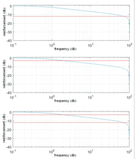
s(x). Proposed algorithm is composed of two stages – decomposition and reconstruction of the signal, and may be used in order for distribution of various filters. Definition 6. Filter is function which attenuates sig-nal according to frequency value. There are three types of these filters

– lowpass – signal is passed only below particular value,

– highpass – signal is passed only above particular value,

– bandpass – signal is passed only between particular values.

Illustration of these filters is shown in Fig. 1.

Figure 1

(4)

The algorithm assumes distribution of signal into two components – lower and high half of the signal band-width using suitable filters. The author of the algo-rithm proposed to use spline function to decompose (high-pass and low-pass filter). Then, convolution with the signal is applied with Fourier transform. Fil-ter functions are described as

9

�(�) = � ��(�)

��_�_��_(��), (13)

�(�) = exp(��) �(� � �)��, (14)

�� = �� exp(��) �� , (15)

� = ��, �� = �∑��,�� ,��. (16)

�� = �� , (17)

��= �� , (18)

(14)

9 �(�) = � ��(�)

��_�_��_(��), (13)

�(�) = exp(��) �(� � �)��, (14)

��= �� exp(��) �� , (15)

� = ��, �� = �∑��,�� ,��. (16)

��= �� , (17)

��= �� , (18)

(15)

where S2n is spline function of third degree.

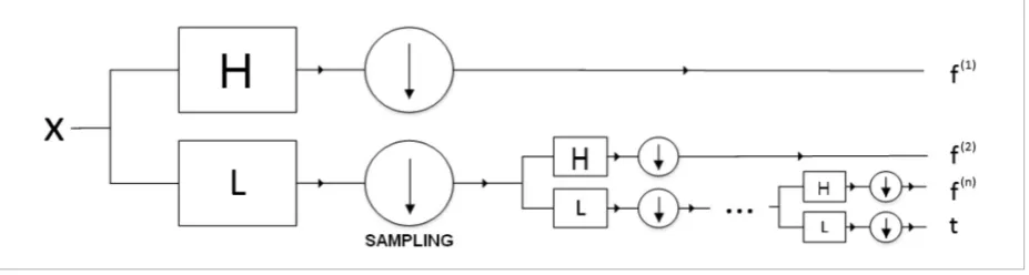
This method uses pyramidal decomposition scheme, that is, in each iteration an additional element or row is added until the last point of analyzed signal. Graphical representation of Mallat’s algorithm is shown in Fig. 2.

3. Heuristic Algorithm

Complex problems require efficient ways for solving, that will not enlarge execution time, consumption of computing power, etc. One of these, inspired by nature, are called heuristic algorithms.

Definition 7.Heuristic algorithm is a method of find-ing optimal solution for given problem, however with condition that returned solution might be improved. In each heuristic algorithm, we assume that individuals are interpreted as points in n-dimensional space and described as x = (x1, x2, ..., xn). Number of individuals in population is defined as k and number of iterations T is constant. Algorithm is based on modeling movement of Figure 2

Graphical representation of Mallat’s algorithm, which helps to speed up wavelet decomposition and reconstruction

individuals for the best adaptation, which is deter-mined by function called fitness function.

3.1 Wolf Search Algorithm

Wolves are individuals that live in herds that try to steer clear of enemies while searching for food. Math-ematical model of behavior of wolves has been de-scribed as a heuristic algorithm by Tang et al. [19] Because of the fact that wolves live in herd, model assumes that the greater the distance, the less attrac-tive is place. Each individual is moving in search for food, movement of which is modeled by

9

�(�) = �_��(�)_{��(��)}, (13)

�(�) = exp(��) �(� � �)��, (14)

��= �� exp(��) �� , (15)

� = ��, �� = �∑��,�� ,��. (16)

��= �� , (17)

��= �� , (18)

(16)

where t is iteration of the algorithm,

9

�(�) = � ��(�)

��_{��(��)}, (13)

�(�) = exp(��) �(� � �)��, (14)

��= �� exp(��) �� , (15)

� = ��, �� = �∑��,�� ,��. (16)

��= �� , (17)

��= �� , (18)

is parameter defining incentive of place,

9

�(�) = �_��(�)_{��(��)}, (13)

�(�) = exp(��) �(� � �)��, (14)

��= �� exp(��) �� , (15)

� = ��, �� = �∑��,�� ,��. (16)

��= �� , (17)

��= �� , (18)

is the closest neighbor of

9

�(�) = �_��(�)_{��(��)}, (13)

�(�) = exp(��) �(� � �)��, (14)

��= �� exp(��) �� , (15)

� = ��, �� = �∑��,�� ,��. (16)

��= �� , (17)

��= �� , (18)

with better value of fitness function and

9

�(�) = � ��(�)

��_�_��_(��), (13)

�(�) = exp(��) �(� � �)��, (14)

��= �� exp(��) �� , (15)

� = ��, �� = �∑��,�� ,��. (16)

��= �� , (17)

��= �� , (18) is ran-dom value in range < 0,1 > and r is distance between these two wolves defined as

9 �(�) = � ��(�)

��_�_��_(��), (13)

�(�) = exp(��) �(� � �)��, (14)

�_��_{= �} � �_{� �}

�exp(��) �� , (15)

� = ��, �� = �∑��,�� ,��. (16)

��= �� , (17)

�_��_{= �} �

�_{� ��,}₍₁₈₎

(17)

The hunt of wolves is defined as stalking process which consists of three phases. The first of them is called initiative stage which is understood as move-ment of individual within his sight in search of a bet-ter place. This step is modeled as

9

�(�) = � ��(�)

��_�_��_(��), (13)

�(�) = exp(��) �(� � �)��, (14)

��= �� exp(��) �� , (15)

� = ��, �� = �∑��,�� ,��. (16)

��= �� , (17)

��= �� , (18)

(18)

(5)

enemy will be in vicinity, modeled by

9

�(�) = � ��(�)

��_�_��_(��), (13)

�(�) = exp(��) �(� � �)��, (14)

�_��_{= �} � �_{� �}

�exp(��) �� , (15)

� = ��, �� = �∑��,�� ,��. (16)

��= �� , (17)

��= �� , (18) (19) where s is step size. The complete algorithm is pre-sented in Algorithm 1.

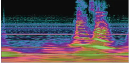
played using energy density. Scaleogram is built on two axes: time representing (OX axis) and scale (axis OY). Each value on such spread-axis corresponds to wavelet coefficients, which are illustrated by different shades of brightness. Another form of visual represen-tation can be done using signal frequency and time domain. Example of scaleogram and visualization of wavelet are illustrated in Fig. 5–7.

4. Feature Extraction

Our method for feature extraction from signal sample is based on idea of extraction information from imag-es. In order to present the signal in graphical form, we use scaleograms and visualization of sound sample in frequency-time domain. Created images become search space in which individuals of a given popula-tion in heuristic algorithm move and search for im-portant information.

4.1 Signal Visualization

One way to visualize wavelet transform for a given signal is scaleogram, where wavelet transform is

dis-Figure 5

Representation of the sentence “Han Solo” by using the scaleogram

Figure 6

Linear representation of the sentence “Han Solo” in frequency-time domain

Figure 7

(6)

4.2 Extraction of Important Information Visualization of signal allows to use it as search space for applied heuristic method. Each individual will cor-respond to coordinates of points represented by pixel. In algorithm we will look for most valuable points (pixels) of scalogram image. In this way, algorithm returns specific set of points, which correspond to contained information (or features) in given sound sample.

In case of scaleogram, the most important information are dark areas, so we use heuristic to search for pixel i.e. using brightness feature. This allows us to define fitness function

10 4. Feature Extraction

Our method for feature extraction from signal sample is based on idea of extraction information from images. In order to present the signal in graphical form, we use scaleograms and visualization of sound sample in frequency-time domain. Created images become search space in which individuals of a given population in heuristic algorithm move and search for important information.

4.1. Signal Visualization

One way to visualize wavelet transform for a given signal is scaleogram, where wavelet transform is displayed using energy density. Scaleogram is built on two axes: time representing (OX axis) and scale (axis OY). Each value on such spread-axis corresponds to wavelet coefficients, which are illustrated by different shades of brightness. Another form of visual representation can be done using signal frequency and time domain. Example of scaleogram and visualization of wavelet are illustrated in Fig. 5-7.

4.2. Extraction of Important Information

Visualization of signal allows to use it as search space for applied heuristic method. Each individual will correspond to coordinates of points represented by pixel. In algorithm we will look for most valuable points (pixels) of scalogram image. In this way, algorithm returns specific set of points, which correspond to contained information (or features) in given sound sample.

Figure 3. Cone, which represents color space to build the model for application in decision support system.

In case of scaleogram, the most important information are dark areas, so we use heuristic to search for pixel i.e. using brightness feature. This allows us to define fitness function

��(�) =�(�)��(�)_� , (18) where �(�) = m�� (�(�), �(�), �(�)) and �(�) =

m�� (�(�), �(�), �(�)) wherein �(∙), �(∙) ��d �(∙)

are related to color components (red, green and blue) of a given pixel. Defined in this way function refers to HSL model from which other properties may be used, like hue defined as

��(�) =

� � � �

� 60°��(�)��(�)�(�)��(�)(mod 6)� �� (�) = �(�)

60°_��(�)��(�)

�(�)��(�)� �� (�) = �(�)

60°_��(�)��(�)

�(�)��(�)� �� (�) = �(�)

.

(19) The above function characterize property which is perceived as one of basic color components in RGB model. Another function for saturation can be defined as

��(�) =_{��(�)��(�)��}�(�)��(�) . (20) All of these three functions are used in formal description of HSL model, which is in a form of cone representing colors as compositions of three

Figure 2. Graphical representation of Mallat’s algorithm, which helps to speed up wavelet decomposition and reconstruction.

Commented [MV1]: Jei galite, po šios pastraipos įdėkite gale esančias Figure 5, 6 ir 7.

(20)

where

10 4. Feature Extraction

One way to visualize wavelet transform for a given signal is scaleogram, where wavelet transform is displayed using energy density. Scaleogram is built on two axes: timerepresenting (OX axis) and scale (axis OY). Each value on such spread-axis corresponds to wavelet coefficients, which are illustrated by different shades of brightness. Another form of visual representation can be done using signal frequency and time domain.Exampleofscaleogram and visualization of wavelet areillustrated in Fig. 5-7.

4.2. Extraction of Important Information

Visualization of signal allows to use it as search space for applied heuristic method. Each individual will correspond to coordinates of points represented by pixel. In algorithm we will look for most valuable points (pixels) of scalogram image. In this way, algorithm returns specific set of points, which correspond to contained information (or features) in given sound sample.

Figure 3.Cone, which represents color space to build the model for application in decision support system.

In case of scaleogram, the most important information are dark areas, so we use heuristic to search for pixel i.e. using brightnessfeature. This allows usto define fitness function

𝑓𝑓𝑓𝑓1(𝒙𝒙𝒙𝒙) =𝛿𝛿𝛿𝛿(𝒙𝒙𝒙𝒙)+𝜂𝜂𝜂𝜂₂ (𝜋𝜋𝜋𝜋), (18)

where 𝛿𝛿𝛿𝛿(𝒙𝒙𝒙𝒙) = max (𝑅𝑅𝑅𝑅(𝒙𝒙𝒙𝒙),𝐺𝐺𝐺𝐺(𝒙𝒙𝒙𝒙),𝐵𝐵𝐵𝐵(𝒙𝒙𝒙𝒙)) and 𝜂𝜂𝜂𝜂(𝒙𝒙𝒙𝒙) = min (𝑅𝑅𝑅𝑅(𝒙𝒙𝒙𝒙),𝐺𝐺𝐺𝐺(𝒙𝒙𝒙𝒙),𝐵𝐵𝐵𝐵(𝒙𝒙𝒙𝒙)) wherein 𝑅𝑅𝑅𝑅(∙), 𝐺𝐺𝐺𝐺(∙) and 𝐵𝐵𝐵𝐵(∙)

are related to color components (red, green and blue) of agiven pixel. Defined in this way function refers to HSL model from which other properties may be used, like hue defined as

𝑓𝑓𝑓𝑓2(𝒙𝒙𝒙𝒙) =

⎩ ⎪ ⎨ ⎪

⎧ 60°�𝐺𝐺𝐺𝐺𝛿𝛿𝛿𝛿((𝒙𝒙𝒙𝒙𝒙𝒙𝒙𝒙))−𝐵𝐵𝐵𝐵−𝜂𝜂𝜂𝜂((𝜋𝜋𝜋𝜋𝒙𝒙𝒙𝒙))(mod 6)� if 𝛿𝛿𝛿𝛿(𝒙𝒙𝒙𝒙) =𝑅𝑅𝑅𝑅(𝒙𝒙𝒙𝒙) 60°_�𝐵𝐵𝐵𝐵(𝒙𝒙𝒙𝒙)−𝑅𝑅𝑅𝑅(𝒙𝒙𝒙𝒙)

𝛿𝛿𝛿𝛿(𝒙𝒙𝒙𝒙)−𝜂𝜂𝜂𝜂(𝜋𝜋𝜋𝜋)+ 2� if 𝛿𝛿𝛿𝛿(𝒙𝒙𝒙𝒙) =𝐺𝐺𝐺𝐺(𝒙𝒙𝒙𝒙) 60°_�𝑅𝑅𝑅𝑅(𝒙𝒙𝒙𝒙)−𝐺𝐺𝐺𝐺(𝒙𝒙𝒙𝒙)

𝛿𝛿𝛿𝛿(𝒙𝒙𝒙𝒙)−𝜂𝜂𝜂𝜂(𝜋𝜋𝜋𝜋)+ 4� if 𝛿𝛿𝛿𝛿(𝒙𝒙𝒙𝒙) =𝐵𝐵𝐵𝐵(𝒙𝒙𝒙𝒙) .

(19) The above function characterize property which is perceived as one of basic color components in RGB model. Another function for saturation can be defined as

𝑓𝑓𝑓𝑓3(𝒙𝒙𝒙𝒙) =₁₋_|_{𝛿𝛿𝛿𝛿}𝛿𝛿𝛿𝛿₍(𝒙𝒙𝒙𝒙_{𝒙𝒙𝒙𝒙})₎−𝜂𝜂𝜂𝜂_{+𝜂𝜂𝜂𝜂}(₍𝜋𝜋𝜋𝜋_{𝜋𝜋𝜋𝜋})₎₋₁_|. (20)

All of these three functions are used in formal description of HSL model, which is in a form of cone representing colors as compositions of three Figure 2.Graphical representation of Mallat’s algorithm,which helps to speed up wavelet decomposition and

reconstruction.

and

10 4. Feature Extraction

Our method for feature extraction from signal sample

is based on idea of extraction information from images.

In order to present the signal in graphical form, we use

scaleograms and visualization of sound sample in

frequency-time domain. Created images become search

space in which individuals of a given population in

heuristic algorithm move and search for important

information.

4.1. Signal Visualization

One way to visualize wavelet transform for a given

signal is scaleogram, where wavelet transform is

displayed using energy density. Scaleogram is built on

two axes: time representing (OX axis) and scale (axis

OY). Each value on such spread-axis corresponds to

wavelet coefficients, which are illustrated by different

shades of brightness. Another form of visual

representation can be done using signal frequency and

time domain. Example of scaleogram and visualization

of wavelet are illustrated in Fig. 5-7.

4.2. Extraction of Important Information

Visualization of signal allows to use it as search space

for applied heuristic method. Each individual will

correspond to coordinates of points represented by

pixel. In algorithm we will look for most valuable

points (pixels) of scalogram image. In this way,

algorithm returns specific set of points, which

correspond to contained information (or features) in

given sound sample.

Figure 3.

Cone, which represents color space to build

the model for application in decision support system.

In case of scaleogram, the most important

information are dark areas, so we use heuristic to search

for pixel i.e. using brightness feature. This allows us to

define fitness function

�

(�) =

�(�)��(�)_�

,

(18)

where

�(�) = m�� (�(�), �(�), �(�))

and

�(�) =

m�� (�(�), �(�), �(�))

wherein

�(∙), �(∙) ��d �(∙)

are related to color components (red, green and blue) of

a given pixel. Defined in this way function refers to

HSL model from which other properties may be used,

like hue defined as

�

(�) =

�

� 60

°

�

�(�)��(�)�(�)��(�)

(mod 6)� �� (�) = �(�)

60

°

_�

�(�)��(�)

� �� (�) = �(�)

60

°

_�

�(�)��(�)

� �� (�) = �(�)

.

(19)

The above function characterize property which is

perceived as one of basic color components in RGB

model. Another function for saturation can be defined

as

�

(�) =

_{��(�)��(�)��}�(�)��(�)

. (20)

All of these three functions are used in formal

description of HSL model, which is in a form of cone

representing colors as compositions of three

Figure 2. Graphical representation of Mallat’s algorithm, which helps to speed up wavelet decomposition and reconstruction.

Commented [MV1]: Jei galite, po šios pastraipos įdėkite gale esančias Figure 5, 6 ir 7.

= min (R(x), G(x), B(x)) wherein R(∙), G(∙) and B(∙) are re-lated to color components (red, green and blue) of a given pixel. Defined in this way function refers to HSL model from which other properties may be used, like hue defined as

10

4. Feature Extraction

One way to visualize wavelet transform for a given signal is scaleogram, where wavelet transform is displayed using energy density. Scaleogram is built on

��(�) =

� � � �

� 60°��(�)��(�)�(�)��(�)(mod 6)� �� (�) = �(�)

60°_��(�)��(�)

�(�)��(�)� �� (�) = �(�)

60°_��(�)��(�)

�(�)��(�)� �� (�) = �(�)

.

��(�) =_{��(�)��(�)��}�(�)��(�) . (20)

Figure 2. Graphical representation of Mallat’s algorithm, which helps to speed up wavelet decomposition and

reconstruction.

(21)

The above function characterize property which is per-ceived as one of basic color components in RGB model. Another function for saturation can be defined as

10 4. Feature Extraction

One way to visualize wavelet transform for a given signal is scaleogram, where wavelet transform is displayed using energy density. Scaleogram is built on

��(�) =

� � � �

� 60°��(�)��(�)�(�)��(�)(mod 6)� �� (�) = �(�) 60°_��(�)��(�)

�(�)��(�)� �� (�) = �(�) 60°_��(�)��(�)

�(�)��(�)� �� (�) = �(�) .

��(�) =_{��(�)��(�)��}�(�)��(�) . (20)

Figure 2. Graphical representation of Mallat’s algorithm, which helps to speed up wavelet decomposition and

reconstruction.

(22)

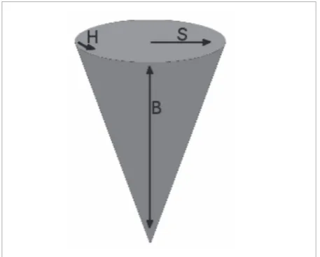
All of these three functions are used in formal descrip-tion of HSL model, which is in a form of cone repre-senting colors as compositions of three components: hue, saturation and brightness (also called lightness). The cone representation is shown in Fig. 3.

Defined fitness function can be used to extract infor-mation from image. Fitness function is a flexible ele-ment of proposed approach, so we can modify it to various initial conditions. Found points in image can form a feature vector as follows

[��(��), ��(��), . . , ��(��)]. (21)

�∑� �_�

�� (��), ∑��_��(��), . . , ∑��_��(��)�, (22)

�(��) = ∑ �� ∗�, (23)

�� = �_��. (24) (23)

Figure 3

Cone, which represents color space to build the model for application in decision support system

This type of vector will represent specific values in terms to selected fitness function . Number of elements depends on selection of individuals in heuristic algo-rithm. Proposed heuristic returns only n best individu-als. The greater number of features, the higher should be number of individuals in predetermined population.

5. Speaker Recognition as Testing Tool

Proposed solution for feature extraction from graph-ical representation of audio signal is efficient for voice verification or recognition. In this section, we present two examples of verification methods that can benefit from proposed approach to feature ex-traction.

5.1 Template Matching

One of the easiest and most popular methods of com-parison of two vectors is their pattern matching. Pat-tern will be called vector formed by k samples, where each value is averaged in suitable way and some errors of measurement are specified. Pattern vector can be determined in various way, for example, arithmetic mean of k samples

[��(��), ��(��), . . , ��(��)]. (21)

�∑� _��

�� (��), ∑��_��(��), . . , ∑��_��(��)�,

�(��) = ∑ �� ∗�, (23)

�� = �_��. (24)

(7)

where

[��(��), ��(��), . . , ��(��)]. (21)

�∑� �_�

�� (��), ∑��_��(��), . . , ∑��_��(��)�,

�(��) = ∑ �� ∗�, (23)

�� = ��_��. (24)

is value f (x1) for j-th sample. For this vector, comparison must be evaluated relative to error, be-cause it is unlikely to achieve identical results for two different samples. For this purpose, we propose to construct error function δ (∙) dependent on all vari-ables in vectors as follows

[��(��), ��(��), . . , ��(��)]. (21)

�∑� �_�

�� (��), ∑��_��(��), . . , ∑��_��(��)�,

�(��) = ∑ �� ∗�, (23)

�� = �_��. (24)

(25)

where

11 5. Speaker Recognition as Testing Tool

Proposed solution for feature extraction from graphical representation of audio signal is efficient for voice verification or recognition. In this section, we present two examples of verification methods that can benefit from proposed approach to feature extraction.

where �� [��(��)� ��(��)� � � � ��(��)] and �� indicate j -th element in -this vector. As ��∗ , we denote pattern vector described in Eq. (22) and ‖∙‖ is function which can be described in any way satisfying condition ‖∙‖� � � [�� ). In this discussion, we assume that this function is described in the following way

Table 1. The obtained accuracy of the described feature extraction meth consisting of 200 individuals.

Method _functionFitness Population Number of the best ones

Classified samples

Accuracy Correctly Incorrectly

Measurement error with respect to Eq. (24)

Eq. (18) 200 30 ₁₆₃ 37 81,5%

Eq. (19) 200 30 179 21 89,5%

Eq. (20) 200 30 145 55 72,5%

Interval method with respect to Eq. (25)

Eq. (18) 200 30 176 24 88%

Eq. (19) 200 30 165 35 82,5%

Eq. (20) 200 30 147 53 73,5%

Table 2. The obtained accuracy of the described feature extraction method in the speaker recognition application for population consisting of 300 individuals.

Accuracy Correctly Incorrectly

Eq. (18) 300 45 158 42 79%

Eq. (19) 300 45 180 20 90%

Eq. (20) 300 45 105 95 52,5%

Eq. (18) 300 45 168 32 84%

Eq. (19) 300 45 166 34 83%

Eq. (20) 300 45 164 36 82%

and

[��(��), ��(��), . . , ��(��)]. (21)

�∑� _��

�� (��), ∑��_��(��), . . , ∑��_��(��)�,

�(��) = ∑ �� ∗�, (23)

�� = �_��. (24) indicate j-th el-ement in this vector. As

[��(��), ��(��), . . , ��(��)]. (21)

�∑� �_�

�� (��), ∑��_��(��), . . , ∑��_��(��)�,

�(��) = ∑ �� ∗�, (23)

�� = �_��. (24)

, we denote pattern vector described in Eq. (22) and

where �� [��(��)� ��(��)� � � � ��(��)] and �� indicate j-th element in j-this vector. As ��∗ , we denote pattern

vector described in Eq. (22) and ‖∙‖ is function which

can be described in any way satisfying condition ‖∙‖� � � [�� ). In this discussion, we assume that this function is described in the following way

Method _functionFitness Population Number of the

best ones

Accuracy

Correctly Incorrectly

Eq. (18) 200 30 163 37 81,5%

Eq. (19) 200 30 179 21 89,5%

Eq. (20) 200 30 145 55 72,5%

Eq. (18) 200 30 176 24 88%

Eq. (19) 200 30 165 35 82,5%

Eq. (20) 200 30 147 53 73,5%

Method _functionFitness Population Number of the

best ones

Accuracy

Eq. (18) 300 45 158 42 79%

Eq. (19) 300 45 180 20 90%

Eq. (20) 300 45 105 95 52,5%

Eq. (18) 300 45 168 32 84%

Eq. (19) 300 45 166 34 83%

Eq. (20) 300 45 164 36 82%

is function which can be described in any way satisfying condition

where �� [��(��)� ��(��)� � � � ��(��)] and �� indicate j -th element in -this vector. As ��∗ , we denote pattern vector described in Eq. (22) and ‖∙‖ is function which can be described in any way satisfying condition ‖∙‖� � � [�� ). In this discussion, we assume that this function is described in the following way

Accuracy

Eq. (18) 200 30 ₁₆₃ 37 81,5%

Eq. (19) 200 30 179 21 89,5%

Eq. (20) 200 30 145 55 72,5%

Eq. (18) 200 30 176 24 88%

Eq. (19) 200 30 165 35 82,5%

Eq. (20) 200 30 147 53 73,5%

Accuracy

Eq. (18) 300 45 158 42 79%

Eq. (19) 300 45 180 20 90%

Eq. (20) 300 45 105 95 52,5%

Eq. (18) 300 45 168 32 84%

Eq. (19) 300 45 166 34 83%

Eq. (20) 300 45 164 36 82%

In this discussion, we assume that this function is de-scribed in the following way

[��(��), ��(��), . . , ��(��)]. (21)

�∑� �_�

�� (��), ∑��_��(��), . . , ∑��_��(��)�,

�(��) = ∑ �� ∗�, (23)

�� = �_��. (24) (26)

Comparison of two vectors will consist of two stages. In the first one, error value is calculated by Eq. (25) and in next one, these value is verified within range of acceptance, which will be adjusted based on value of this vector and error function for a particular problem. Another example is creation of two vectors, which contain the most diverging from each other

�� min��,…,�� _(�

�)] , min_{��,…,�}� ��(��)] , … , min_{��,…,�}� ��(��)]�

� max ��,…,��

�_(�

�)] , max_{��,…,�}� ��(��)] , … , max_{��,…,�}� ��(��)]� . (27)

This approach is indicated that if the value is not be-tween minimum and maximum of variables, the vector

is discarded. In the case of too many restrictions on ac-ceptance, both vectors can be extended to a certain per-centage of error adjusted in relation to given problem.

6. Experiments

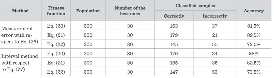
Measurement accuracy and effectiveness of proposed method was analyzed using 200 audio samples with the sentence “Han Solo”. The tests were performed for both presented methods of speaker recognition. Ex-periments were performed for population of 200 and 300 individuals, where only the top 15% of them have been returned. Number of selected individuals forced length of vectors as 30 and 45. As fitness function three variants were selected described by Eq. (20)–(22). For these parameters, all samples were processed by each method. Thereafter, each sample was tested for these patterns and specific fitness function. Results of measurements are shown in Tab. 1 and Tab. 2. For first examined method with error measures, accuracy for almost all fitness functions becomes worse with increasing amount of individuals. Accuracy for second method remains at almost constant level, about 83% for each of fitness functions.

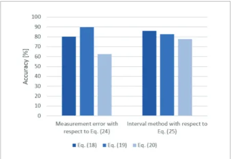
Randomness of heuristic algorithm and sound samples influence operation of methods so we can not predict constant accuracy for other functions. Of course tests were carried out on a small number of samples with short recording time so accuracy of these results is very high. Average accuracy of methods in term of applied fitness function is shown in Fig. 4. For used functions the best

Table 1

The obtained accuracy of the described feature extraction method in the speaker recognition application for population consisting of 200 individuals

Method _functionFitness Population Number of the _{best ones} Classified samples Accuracy

Measurement error with re-spect to Eq. (26)

Eq. (20) 200 30 163 37 81,5%

Eq. (21) 200 30 179 21 89,5%

Eq. (22) 200 30 145 55 72,5%

Eq. (20) 200 30 176 24 88%

Eq. (21) 200 30 165 35 82,5%

(8)

results were obtained for Eq. (21) and the worst for Eq. (22). The reason for differences is primarily a function, and more specifically adaptation to search for specific features. For graphical representation of audio signal, specific areas of images were searched and selection of most precise fitness function im-proves results.

ples. The use of heuristic algorithm allows to detect specific, unique (because of randomness of popula-tion) sequence of positions in images what can be used in real-time recognition, which could find application in many practical purposes. Especially in large corpo-rations where access is granted under certain identi-ty verification conditions.

In corporations we can use a sample mechanism, to collect samples from workers, which will be stored in a database system from which trained architectures can extract samples for verification. A user coming to work can be verified by ad-hoc recording of the voice, which will be forwarded to the verification system. Result is returned to entrance, where user gain access or is denied from entering.

Proposed solution depends on fitness function what allows for feature extraction not only of audio signals but also all kinds of signals, but also many other ob-jects like 2D graphics. Interesting approach may be the usage of other transforms as well as fitness func-tions. In future research we would like to examine the impacts of application of various heuristic algorithms. Additionally, use of similar solutions to other classi-fiers could be attractive in terms of accuracy.

Acknowledgments

Authors acknowledge contribution to this project from the “Diamond Grant 2016” No. 0080/DIA/2016/45 funded by the Polish Ministry of Science and Higher Education.

Method _functionFitness Population _{of the best ones}Number Classified samples Accuracy

Eq. (20) 300 45 158 42 79%

Eq. (21) 300 45 180 20 90%

Eq. (22) 300 45 105 95 52,5%

Eq. (20) 300 45 168 32 84%

Eq. (21) 300 45 166 34 83%

Eq. (22) 300 45 164 36 82%

Table 2

The obtained accuracy of the described feature extraction method in the speaker recognition application for population consisting of 300 individuals

Figure 4

Average accuracy of detected features during verification by application of various fitness functions

7. Conclusions

(9)

sam-Information Technology and Control 2017/3/46 380

References

1. Besacier, L., Bernard, E., Karpov, A., Schultz, T. Auto-matic Speech Recognition for Under-Resourced Lan-guages: A Survey. Speech Communication, 2014, 85-100. https://doi.org/10.1016/j.specom.2013.07.008

2. Brociek, R., Słota, D. Application and Comparison of Intelligent Algorithms to Solve the Fractional Heat Con-duction Inverse Problem. Information Technology and Control, 2016, 45(2), 184-194. https://doi.org/10.5755/ j01.itc.45.2.13716

3. Costa, Y. M., Oliveira, L. S., Carlos, C. N. An Evaluation of Convolutional Neural Networks for Music Classification Using Spectograms. Applied Soft Computing, 2017, 52, 28-38. https://doi.org/10.1016/j.asoc.2016.12.024 4. Chodarev, S., Kollar, J. Extensible Host Language for

Domain-Specific Languages. Computing and Informat-ics, 2016, 35(1), 84-110.

5. Damaševičius, R., Maskeliūnas, R., Venčkauskas, A., Woźniak, M. Smartphone User Identity Verification Using Gait Characteristics. Symmetry, 2016, 8(10), 100. https://doi.org/10.3390/sym8100100

6. Gabryel, M. The Bag-of-Features Algorithm for Practical Applications Using the MySQL Database. Lecture Notes in Computer Science, 2016, 9693, 635-646. https://doi. org/10.1007/ 978-3-319-39384-1_56

7. Gabryel, M. A Bag-of-Features Algorithm for Applica-tions Using a NoSQL Database. CommunicaApplica-tions in Computer and Information Science, 2016, 639, 332-343. https://doi.org/10.1007/978-3-319-46254-7_26 8. Griffiths, K. R., Hicks, B. J., Keogh, P. S., Shires, D.

Wave-let Analysis to Decompose a Vibration Simulation Signal to Improve Pre-distribution Testing of Packaging. Me-chanical Systems and Signal processing, 2016, 76, 780-795. https://doi.org/10.1016/j.ymssp.2015.12.035 9. Haar, A. Zur Theorie der Orthogonalen

Funktionensys-teme. Mathematische Annalen, 69(3), 1910, 331-371. https://doi.org/10.1007/BF01456326

10. Kameoka, H. Non-negative Matrix Factorization and Its Variants for Audio Signal Processing. Applied Matrix and Tensor Variate Data Analysis. Springer Japan, 2016, 23-50. https://doi.org/10.1007/978-4-431-55387-8_2 11. Korytkowski, M., Rutkowski, L. Fast Image Classification

by Boosting Fuzzy Classifiers. Information Sciences, 2016, 327, 175-182. https://doi.org/10.1016/j.ins.2015. 08.030 12. Martisius, I., Damasevicius, R. A Prototype {SSVEP}

Based Real Time {BCI} Gaming System.

Computation-al Intelligence and Neuroscience, 2016, 639, 3861425:1-3861425:15. //doi.org/ 10.1155/2016/3861425

13. Nowicki, R. K., Scherer, R., Rutkowski, L. Novel Rough Neural Network for Classification with Missing Data. 21st International Conference on Methods and Models in Automation and Robotics (MMAR), 2016, 820-825. https://doi.org/10.1109/MMAR.2016.7575243

14. Porubaen, J., Bačíková, M., Chodarev, S., Nosal, M. Teaching Pragmatic Model-Driven Software Develop-ment. Computer Science & Information Systems, 2015, 12(2), 683-705. https://doi.org/10.2298/CSI-S140107022P

15. Scherer, R., Rutkowski, L. A Fuzzy Relational System with Linguistic Antecedent Certainty Factors. Interna-tional Conference on Neural Networks and Soft Com-puting, 2003, 563-569. https://doi.org/10.1007/978-3-7908-1902-1_86

16. Sebastian, J., Kumar, M., Murthy, H. A. An Analysis of the High Resolution Property of Group Delay Function with Applications to Audio Signal Processing. Speech Communication, 2016, 81, 42-53. https://doi.org/10.1016/ j.specom.2015.12.008

17. Słota, D., Brociek, R. Application of Real Ant Colony Op-timization Algorithm to Solve Space Fractional Heat Conduction Inverse Problem. Communications in Com-puter and Information Science, 2016, 639, 369-379. https://doi.org/10.1007/ 978-3-319-46254-7_29 18. Sulír, M., Nosáľ, M., Porubän, J. Recording Concerns in

Source Code Using Annotations. Computer Languages, Systems & Structures, 2016, 46, 44-65. https://doi. org/10.1016/j.cl.2016.07.003

19. Tang, R., Fong, S., Yang, X. S., Deb, S. Wolf Search Algo-rithm with Ephemeral Memory. 7th International Con-ference on Digital Information Management, 2012, 165-172. https://doi.org/10.1109/ICDIM.2012.6360147 20. Terada, H., Makino, K., Nishizaki, H., Yanase, E.,

Suzu-ki, T., Tanzawa, T. Positioning Control of a Micro Manip-ulation Robot Based on Voice Command Recognition for the Microscopic Cell Operation. Advances in Mechanism Design II, Springer International Publishing, 2017, 73-79. 21. Ubhayarantne, L., Pereira, M. P., Xiang, Y., Rolfe, B. F.

The Use of Wavelet Transformation in Conjunction with a Heuristic Algorithm as a Tool for Feature Extraction from Signals

The Use of Wavelet Transformation

in Conjunction with a Heuristic

Algorithm as a Tool for Feature

Extraction from Signals

Dawid Połap and Marcin Woźniak

1. Introduction

2. Wavelet Transform

8

8

�

� � �). (2)

�(�) = 2sinc(2�) − sinc(�) =

,

(3)

sinc(�) = �

��� � � 0

� ��� � = 0

. (4)

�

� �

�, (5)

where �

� is called core of transformation, and � �

0

.

�

�� � �,

(6)

� �(�)�� = 0

. (7)

�̂

(�, �) =

� �(�)� �

�

��. (8)

�(�) =

�

� �̂�

(�, �)� �

�

����

(9)

�̂�(�, �) = � �

(�)�(�)��

. (10)

�

= �

� �

� , �, � � �

. (11)

��

(�)�(�)��.

(12)

�(�) = �

∑ ∑ ���(�, �)��,�

(�)

, (12)

8

�

(�) = �(2

� � �).

(2)

�(�) = 2sinc(2�) − sinc(�) =

,

(3)

sinc(�) = �

��� � � 0

� ��� � = 0

. (4)

�

(�) =

� �

�

, (5)

where

�

�

is called core of transformation, and

� �

_{� � �). (2)}

�� 0

� �� = 0

�� ,

��

∑ ∑ ��(�, �)��,�

�� 0

� �� = 0

�� ,

��