Efficient Case Study for Image Edge Gradient Based Detectors - Sobel, Robert Cross, Prewitt and Canny

(1)

Efficient Case Study for Image Edge Gradient Based Detectors - Sobel,

Robert Cross, Prewitt and Canny

B.RAMESH NAIDU

Associate Professor, Department of CSE, AITAM, Tekkali, Srikakulam, AP, INDIA.

P.LAKSHMAN RAO

Assistant Professor, Department of MCA, AITAM, Tekkali, Srikakulam, AP, INDIA.

Prof. M.S.PRASAD BABU

Department of CS & SE,

Andhra University, Visakhapatnam, AP, INDIA

K.V.L. BHAVANI

Sr. Assistant Professor, Department of ECE, AITAM, Tekkali, Srikakulam, AP, INDIA.

Abstract — In this paper we focused on the image processing techniques mainly Image enhancement and Feature extraction. Image enhancement is one of the most important issues in low-level image processing. Contrast enhancement (CE) is used widely in image processing. We implement one of the most popular CE methods called histogram equalization (HE). The HE uses the cumulative distribution function (CDF) of a given image as a mapping from the given image to the enhanced image; enhanced image follows the uniform distribution of histogram over the dynamic range of all intensities. It is a widely used contrast enhancement method in a variety of applications due to its simple function and effectiveness. Edges are important features in an image since they represent significant local intensity changes. They provide important clues to separate regions within an object. Edge detection on an image significantly reduces the amount of data and filters out useless information, while preserving the important structural properties in an image. We implemented edge Gradient based detectors- Sobel, Robert Cross, Prewitt and also Canny edge detector.

Keywords — Image Processing, Contrast enhancement, histogram equalization, cumulative distribution function, edge Gradient based detectors.

I. I

NTRODUCTION

Image processing modifies pictures to improve their quality (enhancement, restoration), extract information (analysis, recognition), and change their structure (composition, image editing). Images can be processed by optical, photographic, and electronic means, but image processing using digital computers is the most common method because digital methods are fast, flexible, and precise[1,2]. Image processing is the field of signal processing where both the input and output signals are images. Images can be thought of as two-dimensional signals via a matrix representation. The brief definition of image processing is the ability to retrieve information from images. This is achieved by, first transforming the image into a data set. Mathematical operations can be done on this new format. Different kinds of information are retrieved by the different operations that are performed on the data set. It is important to note that the reverse, constructing an image from data, is also image processing.

Image processing is used in many different fields. In medicine (the ultrasound machine, X-ray machine), astronomy (Hubble’s telescope taking photographs in X-rays, Gamma rays, Infrared) and military (image maps used in ground hugging missiles), these are just a few of the fields in which image processing is widely used. Image processing is also used in everyday items (digital cameras) to mission critical systems[2,3].

A. Image Processing Techniques:

The main techniques in image processing are:

Image enhancement is the improvement of digital image quality (wanted e.g. for visual inspection or for machine analysis), without knowledge about the source of degradation. If the source of degradation is known, one calls the process as image restoration. Both are iconical processes, viz. input and outputs are images.

Image segmentation refers to the process of partitioning a digital image into multiple segments (sets of pixels). The goal of segmentation is to simplify and/or change the representation of an image into something that is more meaningful and easier to analyze.

Feature extraction in pattern recognition and in image processing, is a special form of dimensionality reduction. When the input data to an algorithm is too large to be processed and it is suspected to be notoriously redundant (much data, but not much information) then the input data will be transformed into a reduced representation set of features (also named features vector). Transforming the input data into the set of features is called features extraction.

Image Morphing is a special effect in motion pictures and animations that changes (or morphs) one image into another through a seamless transition. Most often it is used to depict one person turning into another through technological means or as part of a fantasy or surreal sequence.

Image analysis is the extraction of meaningful information from images; mainly from digital images by means of digital image processing techniques. Image analysis tasks can be as simple as reading bar coded tags or as sophisticated as identifying a person from their face.

(2)

an excellent image analysis apparatus, especially for extracting higher-level information, and for many applications including medicine, security, and remote sensing. In this paper the image processing techniques Image enhancement and Feature Extraction are implemented and these techniques[4,5,6,7]

II. I

MAGE

E

NHANCEMENT

Image enhancement is the improvement of digital image quality (wanted e.g. for visual inspection or for machine analysis), without knowledge about the source of degradation. If the source of degradation is known, one calls the process image restoration. Image enhancement improves the quality (clarity) of images for human viewing. Removing blurring and noise, increasing contrast, and revealing details are examples of enhancement operations[7,8,9].

For example, an image might be taken of an endothelial cell, which might be of low contrast and somewhat blurred. Reducing the noise and blurring and increasing the contrast range could enhance the image. The original image might have areas of very high and very low intensity, which mask details.

An adaptive enhancement algorithm reveals these details. Adaptive algorithms adjust their operation based on the image information (pixels) being processed. In this case the mean intensity, contrast, and sharpness (amount of blur removal) could be adjusted based on the pixel-intensity statistics in various areas of the image. Image processing technology is used by planetary scientists to enhance images of Mars, Venus, or other planets. Doctors use this technology to manipulate CAT scans and MRI

images. The aim of image enhancement is to improve the interpretability or perception of information in images for human viewers, or to provide `better' input for other automated image processing techniques[9,10,11].

B. Histogram equalization

Histogram: A histogram can represent any number of things, since its purpose is to graphically summarize the distribution of a single-variable set of data .Each specific use targets some different features of histogram graphs. When viewing an image represented by a histogram, what we are really doing is analyzing the number of pixels (vertically) with a certain frequency (horizontally). In essence, an equalized image is represented by an equalized histogram where the number of pixels is spread evenly over the available frequencies[11,12].

The histogram in the context of image processing is the operation by which the occurrences of each intensity value in the image is shown. Normally, the histogram is a graph showing the number of pixels in an image at each different intensity value found in that image. For an 8-bit grayscale image there are 256 different possible intensities, and so the histogram will graphically display 256 numbers showing the distribution of pixels amongst those grayscale values. The main property of histogram is that the sum of all values in the histogram equals the total number of pixels in the image[13,14].

An overexposed image is defined as an image in which there are an excessive number of pixels with a high pixel frequency, while there is a shortage of low frequencies (Figure 1). The data in a histogram representing an overexposed image therefore is not spread evenly over the horizontal axis, instead skewing non-symmetrically to the absolute right edge of the graph (Figure 1)

Fig.1. An overexposed image & its Histogram Usually, when the number of pixels with very high pixel

frequencies is so high – as shown in the example – it means that some image data has been lost; it is then impossible to restore detail in areas where the pixel

(3)

C. Histogram Equalization algorithm working

procedure

Histogram Equalization is a contrast enhancement technique. It improves contrast and the goal of it is to obtain a uniform histogram. Histogram equalization is the technique by which the dynamic range of the histogram of an image is increased. It assigns the intensity values of pixels in the input image such that the output image contains a uniform distribution of intensities. This technique can be used on a whole image or just on a part of an image. Histogram equalization redistributes intensity distributions. If the histogram of any image has many peaks and valleys, it will still have peaks and valley after equalization, but peaks and valley will be shifted. In histogram equalization, each pixel is assigned a new intensity value based on the previous intensity level[15,16].

i. Grey scale manipulation

The simplest form of operation is when the operator T only acts on a 1×1 pixel neighborhood in the input image, that is Fˆ(x,y) only depends on the value of F at (x,y). This is a grey scale transformation or mapping.

The simplest case is thresholding where the intensity profile is replaced by a step function, active at a chosen threshold value. In this case any pixel with a grey level below the threshold in the input image gets mapped to 0 in the output image. Other pixels are mapped to 255. There are many other grayscale transformations such as darkening, lightening, high contrast, low contrast, etc. As we know, Histogram equalization is a common technique for enhancing the appearance of images. Suppose we have an image which is predominantly dark. Then its histogram would be skewed towards the lower end of the grey scale and all the image detail is compressed into the dark end of the histogram. If we could ‘stretch out' the grey levels at the dark end to produce a more uniformly distributed histogram then the image would become much clearer.

Fig.3. The original image and its histogram, and the equalized versions. Both images are quantized to 64 grey levels.

Histogram equalization involves finding a grey scale transformation function that creates an output image with a uniform histogram (or nearly so).Determining the grey

(4)

in the input image F to grey values s = T(r) in the transformed image Fˆ. It is assumed that

 T is single valued and monotonically increasing, and

 0≤ T(r) ≤1for 0≤r ≤1

The inverse transformation from s to r is given by r = T -1_(s).

If one takes the histogram for the input image and normalizes it so that the area under the histogram is 1, we have a probability distribution for grey levels in the input image Pr(r). If we transform the input image to get s = T(r)

Probability distribution Ps(s) from probability theory it turns out that:

Ps(s) = Pr(r). ds dr

Where r = T-1(s). Consider the transformation

S = T(r) = rPr(w)dw 0



This is the cumulative distribution function of r. Using this definition of T we see that the derivative of s with respect to r is

dr ds

= Pr(r) Substituting this back into the expression for Ps, we get Ps(s)= Pr(r) 1

) Pr(

1 _

r for all s, where 0≤ s ≤ 1.Thus,Ps(s) is now a uniform distribution function, which is desired.

ii. Discrete Formulation

We first need to determine the probability distribution of grey levels in the input image. Now Pr(r)=

N

nk

_Where

n

k

is the number of pixels having grey level k,

and N is the total number of pixels in the image.

The transformation now becomes sk= T(rk) =



k_ i N n 0 1 =



 k

i 0Pr(ri) Note that0 ≤ rk ≤ 1 , the index k=0, 1, 2 ,……,255, and 0 ≤sk≤ 1 .The values of skwill have to be scaled up by 255 and rounded to the nearest integer so that the output values of this transformation will range from 0 to 255. Thus the discretization and rounding of sk to the nearest integer will mean that the transformed image will not have a perfectly uniform histogram.

III. F

EATURE

E

XTRACTION

D. Image feature

There is no exact definition of what constitutes a feature, and the exact definition often depends on the problem or the type of application. Given that, a feature is defined as an "interesting" part of an image, and features are used as a starting point for many computer vision algorithms. Since features are used as the starting point and main primitives for subsequent algorithms, the overall algorithm will often only be as good as its feature detector. Consequently, the desirable property for a feature detector

is repeatability: whether or not the same feature will be detected in two or more different images of the same scene.

Feature detection is a low-level image processing operation. That is, it is usually performed as the first operation on an image, and examines every pixel to see if there is a feature present at that pixel. If this is part of a larger algorithm, then the algorithm will typically only examine the image in the region of the features. As a built-in pre-requisite to feature detection, the built-input image is usually smoothed by a Gaussian kernel in a scale-space representation and one or several feature images are computed, often expressed in terms of local derivative operations.

When feature detection is computationally expensive and there are time constraints, a higher level algorithm may be used to guide the feature detection stage, so that only certain parts of the image are searched for features.

Where many computer vision algorithms use feature detection as the initial step, so as a result, a very large number of feature detectors have been developed. These vary widely in the kinds of feature detected, the computational complexity and the repeatability.

E. Feature Extraction

Once features have been detected, a local image patch around the feature can be extracted. This extraction may involve quite considerable amounts of image processing. The result is known as a feature descriptor or feature vector. Among the approaches that are used to feature description, one can mention N-jets and local histograms (see scale-invariant feature transform for one example of a local histogram descriptor). In addition to such attribute information, the feature detection step by itself may also provide complementary attributes, such as the edge orientation and gradient magnitude in edge detection and the polarity and the strength of the blob in blob detection.

Edge detection is a terminology in image processing and computer vision, particularly in the areas of feature detection and feature extraction, to refer to algorithms which aim at identifying points in a digital image at which the image brightness changes sharply or more formally has discontinuities.

i. Purpose: The purpose of detecting sharp changes in image brightness is to capture important events and changes in properties of the world. It can be shown that under rather general assumptions for an image formation model, discontinuities in image brightness are likely to correspond to:

 Discontinuities in depth,

 Discontinuities in surface orientation,

 Changes in material properties and

 Variations in scene illumination.

(5)

subsequent task of interpreting the information contents in the original image may therefore be substantially simplified.

Unfortunately, however, it is not always possible to obtain such ideal edges from real life images of moderate complexity. Edges extracted from non-trivial images are often hampered by fragmentation, meaning that the edge curves are not connected, missing edge segments as well as false edges not corresponding to interesting phenomena in the image -- thus complicating the subsequent task of interpreting the image data.

ii. Edge properties: The edges extracted from a two-dimensional image of a three-two-dimensional scene can be classified as either viewpoint dependent or viewpoint independent. A viewpoint independent edge typically reflects inherent properties of the three-dimensional objects, such as surface markings and surface shape. A viewpoint dependent edge may change as the viewpoint changes, and typically reflects the geometry of the scene, such as objects occluding one another.

A typical edge might for instance be the border between a block of red color and a block of yellow. In contrast a line (as can be extracted by a ridge detector) can be a small number of pixels of a different color on an otherwise unchanging background. For a line, there may therefore usually be one edge on each side of the line.

Edges play quite an important role in many applications of image processing, in particular for machine vision systems that analyze scenes of man-made objects under controlled illumination conditions. During recent years, however, substantial (and successful) research has also been made on computer vision methods that do not explicitly rely on edge detection as a pre-processing step.

F. Types of image features

i. Edges: Edges characterize boundaries and are therefore a problem of fundamental importance in image processing. Edges in images are areas with strong intensity contrasts–a jump in intensity from one pixel to the next. Edges are points where there is a boundary (or an edge) between two image regions.

In practice, edges are usually defined as sets of points in the image which have a strong gradient magnitude. Furthermore, some common algorithms will then chain high gradient points together to form a more complete description of an edge.

These algorithms may place some constraints on the shape of an edge. Locally, edges have a one dimensional structure.

ii. Corners / interest points: The terms corners and interest points are used somewhat interchangeably and refer to point-like features in an image, which have a local two dimensional structure. The name "Corner" arose since early algorithms first performed edge detection, and then analysed the edges to find rapid changes in direction (corners).

These algorithms were then developed so that explicit edge detection was no longer required, for instance by looking for high levels of curvature in the image gradient. It was then noticed that the so-called corners were also

being detected on parts of the image which were not corners in the traditional sense (for instance a small bright spot on a dark background may be detected). These points are frequently known as interest points, but the term "corner" is used by tradition.

iii. Blobs / regions of interest or interest points Blobs provide a complementary description of image structures in terms of regions, as opposed to corners that are more point-like.

Nevertheless, blob descriptors often contain a preferred point (a local maximum of an operator response or a center of gravity) which means that many blob detectors may also be regarded as interest point operators. Blob detectors can detect areas in an image which are too smooth to be detected by a corner detector.

iv. Ridges: For elongated objects, the notion of ridges is a natural tool. A ridge descriptor computed from a grey-level image can be seen as a generalization of a medial axis. From a practical viewpoint, a ridge can be thought of as a one-dimensional curve that represents an axis of symmetry, and in addition has an attribute of local ridge width associated with each ridge point.

Unfortunately, however, it is algorithmically harder to extract ridge features from general classes of grey-level images than edge-, corner- or blob features. Nevertheless, ridge descriptors are frequently used for road extraction in aerial images and for extracting blood vessels in medical images.

v. Approaches to edge detection: There are many methods for edge detection, but most of them can be grouped into two categories, search-based and zero-crossing based. The search-based methods detect edges by first computing a measure of edge strength, usually a first-order derivative expression such as the gradient magnitude, and then searching for local directional maxima of the gradient magnitude using a computed estimate of the local orientation of the edge, usually the gradient direction.

The zero-crossing based methods search for zero crossings in a second-order derivative expression computed from the image in order to find edges, usually the zero-crossings of the Laplacian or the zero-crossings of a non-linear differential expression, as will be described in the section on differential edge detection following below. As a pre-processing step to edge detection, a smoothing stage, typically Gaussian smoothing, is almost always applied.

The edge detection methods mainly differ in the types of smoothing filters that are applied and the way the measures of edge strength are computed. As many edge detection methods rely on the computation of image gradients, they also differ in the types of filters used for computing gradient estimates in the x- and y-directions.

G. Gradient based edge detection

(6)

the edge. If we calculate the gradient at uniform regions

we end up with a 0 vector which means that there is no

edge pixel.

Fig.4. The gradient and an edge pixel. The circle indicates the location of the pixel. In natural images we usually do not have the ideal

discontinuity or the uniform regions as in the figure and we process the magnitude of the gradient to make a decision to detect the edge pixels. The simplest processing is applying a threshold. If the gradient magnitude is larger than the threshold we decide that the corresponding pixel is an edge pixel.

An edge pixel is described using two important features:

1) Edge strength, which is equal to the magnitude of the gradient

2) Edge direction, which is equal to the angle of the gradient.

Actually, gradient is not defined at all for a discrete function, instead the gradient, which can be defined for the ideal continuous image is estimated using some operators.

H. Canny Edge Detection Algorithm

The Canny edge detection operator was developed by John F. Canny in 1986 and uses a multi-stage algorithm to detect a wide range of edges in images. Most importantly, Canny also produced a computational theory of edge detection explaining why the technique works.

A. Development of the Canny algorithm

Canny's aim was to discover the optimal edge detection algorithm. In this situation, an "optimal" edge detector means:

 Good detection - the algorithm should mark as many real edges in the image as possible.

 Good localization - edges marked should be as close as possible to the edge in the real image.

 Minimal response - a given edge in the image should only be marked once, and where possible, image noise should not create false edges.

The list of criteria to improve current methods of edge detection is the first and most obvious is low error rate. It is important that edges occurring in images should not be missed and that there be NO responses to non-edges. The second criterion is that the edge points be well localized. In other words, the distance between the edge pixels as found by the detector and the actual edge is to be at a minimum.

A third criterion is to have only one response to a single edge. This was implemented because the first 2 were not substantial enough to completely eliminate the possibility of multiple responses to an edge.

Based on these criteria, the canny edge detector first smoothes the image to eliminate and noise. It then finds the image gradient to highlight regions with high spatial derivatives. The algorithm then tracks along these regions and suppresses any pixel that is not at the maximum (nonmaximum suppression).

The gradient array is now further reduced by hysteresis. Hysteresis is used to track along the remaining pixels that have not been suppressed. Hysteresis uses two thresholds and if the magnitude is below the first threshold, it is set to zero (made a nonedge). If the magnitude is above the high threshold, it is made an edge. And if the magnitude is between the 2 thresholds, then it is set to zero unless there is a path from this pixel to a pixel with a gradient above specified threshold.

B. Stages of the Canny algorithm

The Canny Edge Detection Algorithm has the following steps:

 Smooth the image with a Gaussian filter,

 Compute the gradient magnitude and orientation

 Apply nonmaxima suppression to the gradient magnitude,

 Use the Hysterisis thresholding to detect and link edges.

Canny edge detector approximates the operator that optimizes the product of signal-to-noise ratio and localization. The Canny edge detection algorithm is known to many as the optimal edge detector.

Step 1:

(7)

used exclusively in the Canny algorithm.

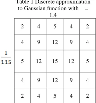
Once a suitable mask has been calculated, the Gaussian smoothing can be performed using standard convolution methods. A convolution mask is usually much smaller than the actual image. As a result, the mask is slid over the image, manipulating a square of pixels at a time. The larger the width of the Gaussian mask, the lower is the detector's sensitivity to noise. The localization error in the detected edges also increases slightly as the Gaussian width is increased. The Gaussian mask used in my implementation is shown below.

Table 1 Discrete approximation to Gaussian function with σ =

1.4

2 4 5 4 2

4 9 12 9 4

5 12 15 12 5

4 9 12 9 4

2 4 5 4 2

Step 2: After smoothing the image and eliminating the noise, the next step is to find the edge strength by taking the gradient of the image. The Sobel operator performs a 2-D spatial gradient measurement on an image. Then, the approximate absolute gradient magnitude (edge strength) at each point can be found.

The Sobel operator uses a pair of 3x3 convolution masks, one estimating the gradient in the x-direction (columns) and the other estimating the gradient in the y-direction (rows). They are shown below:

-1 0 +1

-2 0 +2

-1 0 +1

+1 +2 +1

0 0 0

-1 -2 -1

The magnitude, or EDGE STRENGTH, of the gradient is then approximated using the formula:

| | | | |

|GGx  Gy

Finding the edge direction is trivial once the gradient in the x and y directions are known. However, you will generate an error whenever sum is equal to zero. So in the code there has to be a restriction set whenever this takes

place. Whenever the gradient in the x direction is equal to zero, the edge direction has to be equal to 90 degrees or 0 degrees, depending on what the value of the gradient in the y-direction is equal to. If GY has a value of zero, the edge direction will equal 0 degrees. Otherwise the edge direction will equal 90 degrees. Once the edge direction is known, the next step is to relate the edge direction to a direction that can be traced in an image.

So if the pixels of a 5x5 image are aligned as follows:

× × × × ×

× × a × ×

× × × × ×

Then, it can be seen by looking at pixel "a", there are only four possible directions when describing the surrounding pixels –0 degrees (in the horizontal direction), 45 degrees (along the positive diagonal), 90 degrees (in the vertical direction), or 135 degrees (along the negative diagonal). So now the edge orientation has to be resolved into one of these four directions depending on which direction it is closest to (e.g. if the orientation angle is found to be 3 degrees, make it zero degrees). Think of this as taking a semicircle and dividing it into 5 regions as shown in Figure 5.

Therefore, any edge direction falling within the

yellow range(0 to 22.5 & 157.5 to 180 degrees) is set to 0 degrees.Any edge direction falling in the green range

(22.5 to 67.5 degrees) is set to 45 degrees. Any edge direction falling in theblue range(67.5 to 112.5 degrees) is set to 90 degrees. And finally, any edge direction falling within thered range(112.5 to 157.5 degrees) is set to 135 degrees.

Step 3:

After the edge directions are known, nonmaximum suppression now has to be applied. Nonmaximum suppression is used to trace along the edge in the edge direction and suppress any pixel value (sets it equal to 0) that is not considered to be an edge. This will give a thin line in the output image.

Given estimates of the image gradients, a search is then carried out to determine if the gradient magnitude assumes a local maximum in the gradient direction. So, for example,

 if the rounded angle is zero degrees the point will be considered to be on the edge if its intensity is

(8)

directions,

 if the rounded angle is 90 degrees the point will be considered to be on the edge if its intensity is greater than the intensities in the west and east directions,

 if the rounded angle is 135 degrees the point will be considered to be on the edge if its intensity is greater than the intensities in the north east and south west directions,

 if the rounded angle is 45 degrees the point will be considered to be on the edge if its intensity is greater than the intensities in the north west and south east directions.

This is worked out by passing a 3x3 grid over the intensity map. From this stage referred to as non-maximum suppression, a set of edge points, in the form of a binary image, is obtained. These are sometimes referred to as "thin edges".

Step 4:

Intensity gradients which are large are more likely to correspond to edges than if they are small. It is in most cases impossible to specify a threshold at which a given intensity gradient switches from corresponding to an edge into not doing so. Therefore Canny uses thresholding with hysteresis.

Thresholding with hysteresis requires two thresholds -high and low. Making the assumption that important edges should be along continuous curves in the image allows us to follow a faint section of a given line and to discard a few noisy pixels that do not constitute a line but have produced large gradients. Therefore we begin by applying a high threshold, this marks out the edges. Starting from these, using the directional information derived earlier, edges can be traced through the image. While tracing an edge, we apply the lower threshold, allowing us to trace faint sections of edges as long as we find a starting point.

Once this process is complete we have a binary image where each pixel is marked as either an edge pixel or a non-edge pixel. From complementary output from the edge tracing step, the binary edge map obtained in this way can also be treated as a set of edge curves, which after further processing can be represented as polygons in the image domain.

Finally, hysteresis is used as a means of eliminating streaking. Streaking is the breaking up of an edge contour caused by the operator output fluctuating above and below the threshold. If a single threshold, T1 is applied to an image, and an edge has an average strength equal to T1, then due to noise, there will be instances where the edge dips below the threshold. Equally it will also extend above the threshold making an edge look like a dashed line. To avoid this, hysteresis uses 2 thresholds (say T1 & T2), a high and a low. Any pixel in the image that has a value greater than T1 is presumed to be an edge pixel, and is marked as such immediately. Then, any pixels that are connected to this edge pixel and that have a value greater than T2 are also selected as edge pixels. If you think of

following an edge, you need a gradient of T2 to start but you don't stop till you hit a gradient below T1.

C. Parameters

The Canny algorithm contains a number of adjustable parameters, which can affect the computation time and effectiveness of the algorithm.

 The size of the Gaussian filter: the smoothing filter used in the first stage directly affects the results of the Canny algorithm. Smaller filters cause less blurring, and allow detection of small, sharp lines. A larger filter causes more blurring, smearing out the value of a given pixel over a larger area of the image. Larger blurring radii are more useful for detecting larger, smoother edges - for instance, the edge of a rainbow.

 Thresholds: the use of two thresholds with hysteresis allows more flexibility than in a single-threshold approach, but general problems of thresholding approaches still apply. A threshold set too high can miss important information. On the other hand, a threshold set too low will falsely identify irrelevant information as important. It is difficult to give a generic threshold that works well on all images. No tried and tested approach to this problem yet exists.

IV. I

MPLEMENTATION AND

T

ESTING

I. Implementation

(9)

operators can be represented as a "template", which simplifies the calculations in the java applet.

Canny yielded the best results. This was expected as Canny edge detection accounts for regions in an image. Canny yields thin lines for its edges by using non-maximal suppression.

 Canny also utilizes hysteresis when thresholding. Gradient-based algorithms such as the Prewitt filter have a major drawback of being very sensitive to noise. The size of the kernel filter and coefficients are fixed and cannot be adapted to a given image. An adaptive edge-detection algorithm is necessary to provide a robust solution that is adaptable to the varying noise levels of these images to help distinguish valid image contents from visual artifacts introduced by noise.

 The performance of the Canny algorithm depends heavily on the adjustable parameters, σ, which is the standard deviation for the Gaussian filter, and the threshold values, ‘T1’ and ‘T2’. σ also controls the size of the Gaussian filter. The bigger the value for σ, the larger the size of the Gaussian filter becomes. This implies more blurring, necessary for noisy images, as well as detecting larger edges. As

expected, however, the larger the scale of the Gaussian, the less accurate is the localization of the edge.

 Smaller values of σ imply a smaller Gaussian filter which limits the amount of blurring, maintaining finer edges in the image. The user can tailor the algorithm by adjusting these parameters to adapt to different environments. Canny’s edge detection algorithm is computationally more expensive compared to Sobel, Prewitt and Robert’s operator. However, the Canny’s edge detection algorithm performs better than all these operators under almost all scenarios.

J. Testing

A primary purpose of testing is to detect software failures so that defects may be uncovered and corrected. This is a non-trivial pursuit. Testing cannot establish that a product functions properly under all conditions but can only establish that it does not function properly under specific conditions. The scope of present software testing includes examination of code as well as execution of that code in various conditions as well as examining the quality aspects of code: does it do what it is supposed to do and do what it needs to do. These are shown in Figure 6,7 and 8.

(10)

Fig.8. Canny Edge Detector Output

V. C

ONCLUSION AND

F

UTURE

W

ORK

The most widely used method histogram equalization technique is implemented in paper project which is a global technique in the sense that the enhancement is based on the equalization of the histogram of the entire image. Although it is well recognized, that using only global information is often not enough to achieve good contrast enhancement. To remedy this problem, some authors proposed localized histogram equalization. The adaptivity can usually improve the results but it is computationally intensive even though there are some fast implementations for updating the local histograms. The other extension method is based on fast computation of local min/max/avg maps using a propagation scheme. The quintile based histogram equalization is used for real–time online applications. In this paper we implemented Sobel, Robert Cross, Prewitt and Canny edge detection algorithms were implemented. The Canny algorithm is adaptable to various environments. Its parameters allow it to be tailored to recognition of edges of differing characteristics depending on the particular requirements of a given implementation. Our Experimental results show that our method somehow better when compared to other methods.

R

EFERENCES

[1] Acharya and Ray (2005), “Image Processing: Principles and

Applications”, Wiley-Interscience.

[2] You-yi Zheng, Ji-lai Rao ; Lei Wu(2010), “Edge detection methods in digital image processing” ,ICCSE, pp- 471–473. [3] Bao, P(2002). , “Scale correlation-based edge detection”,

EURASIP-IEEE, pp-345–350.

[4] H. Moon, R. Chellappa, and A. Rosenfeld(2002), “Performance analysis of a simple vehicle detection algorithm,” Image Vis.

Comput., vol. 20, pp.1–13.

[5] R. C. Gonzalez and R. E. Woods, Digital Image Processing, 2nd edition, Prentice Hall, 2001.

[6] W. K. Pratt(2001), Digital Image Processing, 3rd edition, John Wiley and Sons.

[7] Rus. J.C,(1995) “The Image Processing Handbook”, Second Ed.,

Boca Raton, Florida: CRC Press.

[8] Castleman K. R. (1996), “Digital Image Processing”. Second

edition, Englewood Cliffs, New Jersey: Prentice-Hall.

[9] Gonzalez, R. C. and Richard E W (1992), “Digital Image Processing”, Massachusetts: Addison-Wesley.

[10] Lindeberg, T. (1998), "Edge detection and ridge detection with automatic scale selection", International Journal of Computer Vision, 30, 2, pp 117-154.

[11] Ron Ohlander, Keith Price, and D. Raj Reddy (1978): “Picture Segmentation Using a Recursive Region Splitting Method”,

Computer Graphics and Image Processing, volume 8, pp 313-333 [12] Canny, J (1986), “A Computational Approach to Edge Detection”,

IEEE Trans. Pattern Analysis and Machine Intelligence, 8:679-714. [13] Stockham T.G(1972).“Image Processing in the Context of a Visual

Model”.Proc. IEEE, pp. 828–842.

[14] W. K. Pratt.(1991) “Digital Image Processing “Second Ed.. Wiley,

New York.

[15] Boyle R. and Thomas R. (1988) “Computer Vision: A First

Course”, Blackwell Scientific Publications, p 52.

[16] Marr.D. and Hildreth E. C(1980), “Theory of edge detection”.

(11)

A

UTHOR

’

S

P

ROFILE

B.RAMESH NAIDU

Associate Professor, Department of CSE, AITAM, Tekkali, Srikakulam, AP, INDIA.

P.LAKSHMAN RAO

Assistant Professor,

Department of MCA, AITAM, Tekkali, Srikakulam, AP, INDIA.

Prof. M.S.PRASAD BABU

Department of CS & SE, Andhra University, Visakhapatnam, AP, INDIA