of peer-reviewed research and commentary in the population sciences published by the Max Planck Institute for Demographic Research Doberaner Strasse 114 · D-18057 Rostock · GERMANY www.demographic-research.org
DEMOGRAPHIC RESEARCH
VOLUME 6, ARTICLE 6, PAGES 91-144
PUBLISHED 01 MARCH 2002
www.demographic-research.org/Volumes/Vol6/6/
DOI: 10.4054/DemRes.2002.6.6
Tempo-Adjusted Period Parity
Progression Measures, Fertility
Postponement and Completed Cohort
Fertility
Hans-Peter Kohler
José Antonio Ortega
1 Introduction 92
2 Revisiting the Implications of Postponed Childbearing on Period and Cohort Fertility
93
2.1 Intuitive introduction to tempo-adjusted period parity progression measures
93
2.2 Description of period fertility and comparison with adjusted TFR
96
2.3 Continued fertility postponement and cohort fertility
99
3 Adjusting Parity Progression Rates for Tempo and Variance Effects
102
3.1 A parity and age model of fertility 102
3.2 Tempo distortions in childbearing intensities 103
3.3 Measuring and adjusting for tempo changes 110
4 Parity Progression Measures under Alternative Postponement Scenarios
112
4.1 Extrapolation of fertility postponement to future periods
112
4.2 Conditional parity progression probabilities 117
4.3 Conditional parity progression ratios 118
4.4 Conditional cohort mean age at birth 121
5 Using the Model: Measuring Period Fertility and Completing Cohort Fertility
124
5.1 Parity progression measures for measuring period fertility
124
5.2 Completing the fertility of cohorts 125
6 Empirical Implementation 126
Tempo-Adjusted Period Parity Progression Measures, Fertility
Postponement and Completed Cohort Fertility
Hans-Peter Kohler1 Jos´e Antonio Ortega2
Abstract
In this paper we introduce a new set of tempo-adjusted period parity progression mea-sures in order to account for two distinct implications caused by delays in childbearing: tempo distortions imply an underestimation of the quantum of fertility in observed period data, and the fertility aging effect reduces higher parity births because the respective expo-sure is shifted to older ages when the probability of having another child is quite low. Our measures remove the former distortion and provide means to assess the latter aging effect. The measures therefore provide a unified toolkit of fertility indices that (a) facilitate the description and analysis of past period fertility trends in terms of synthetic cohort mea-sures, and (b) allow the projection of the timing, level and distribution of cohort fertility conditional on a specific postponement scenario. Due to their explicit relation to cohort behavior, these measures extend and improve the existing adjustment of the total fertility rate. We apply these methods to Sweden from 1970 to 1999.
1Head of Research Group on Social Dynamics and Fertility, Max Planck Institute for Demographic
Re-search, Doberaner Str. 114, 18057 Rostock, Germany. Tel: +49-381-2081-123, Fax: +49-381-2081-423, Email: [email protected], www: http://user.demogr.mpg.de/kohler.
2Departamento de An´alisis Econ´omico: Econom´ıa Cuantitativa, Universidad Aut´onoma de Madrid,
1
Introduction
Substantial fluctuations in the level of period fertility are often coupled with marked changes in the timing of births. For instance, the postponement of fertility has impor-tantly contributed to the emergence of low and lowest-low fertility in Europe during the 1990s (e.g., Kohler, Billari, and Ortega 2001). These changes in the timing of fertility are of central relevance for demographers interested in the measurement and projection of fertility. On the one hand, future postponement patterns have important implications for cohort fertility and the recuperation of delayed childbearing. On the other hand, past and current delays of childbearing affect the properties and interpretation of standard period fertility measures. In particular, a postponement or anticipation of fertility renders the level of standard period fertility measures different from the level that would have been observed in the absence of tempo changes. These differences are called tempo distortions, and the period fertility level in the absence of tempo distortions is called tempo-adjusted fertility or quantum.
Despite the widespread agreement about the relevance of such tempo distortions, the appropriate way of measuring and adjusting for these effects remains controversial. Bon-gaarts and Feeney (1998, henceforth BF) have proposed an adjusted total fertility rate that measures the total fertility rate that would have been observed in a calendar year if there had been no change in the tempo of fertility during that year. Kohler and Philipov (2001, henceforth KP) have extended this adjustment to include variance effects, i.e., changes in the shape of the fertility schedule in addition to shifts in the mean age. Alternative models for adjusting theT F Rhave also been proposed (e.g., Brass 1990; Le Bras 1997), and virtually all of the above approaches are strongly influenced by the seminal work of Norman Ryder (e.g., Ryder 1964, 1983) (see also the review of the literature on period fertility measures in Ortega and Kohler 2002a).
information about the parity distribution and the completed fertility of cohorts (Kim and Schoen 2000; Ortega and Kohler 2002b; van Imhoff 2001).
In order to overcome this limitation, we develop in this paper tempo-adjusted period parity progression measures that are based on an explicit parity and age fertility model with a long tradition in demographic research (e.g., Park 1976; Quensel 1939; Rallu and Toulemon 1994; Whelpton 1946). These tempo-adjusted parity progression measures provide a new and unified ‘tool-kit’ that can be used for two related purposes. First, they remove tempo distortions and parity composition effects from the observed period fertil-ity pattern and therefore provide an improved indicator of the period quantum of fertilfertil-ity. In particular, our tempo-adjusted period parity progression measures suggest a natural synthetic-cohort measure of period fertility and quantum, denoted period fertility index, that is equal to the total fertility of women who experience the tempo-adjusted period childbearing intensities (or adjusted age-specific parity progression probabilities) during their life-course. Second, our measures allow a demographically correct and consistent projection of the level, timing and distribution of the completed fertility of cohorts who have not finished childbearing, conditional on the future paths of quantum and tempo. We derive these assumptions about future quantum and tempo from observed period fertility patterns. Our methods therefore provide an important input for population projections, and future analyses can combine these methods with stochastic forecasting models that explicitly consider the uncertainty about the future development of quantum and tempo. Moreover, the close relationship between period fertility measurement and cohort pro-jection reduces the traditional distinction between ‘cohort’ and ‘period’ approaches to fertility (e.g., N´ı Bhrolch´ain 1992): our methods provide proper period measures of fer-tility that can be combined with projection scenarios in order to assess the cohort ferfer-tility that results from period fertility patterns.
2
Revisiting the Implications of Postponed Childbearing
on Period and Cohort Fertility
2.1
Intuitive introduction to tempo-adjusted period parity
progres-sion measures
We begin our paper with an intuitive discussion of our methods. The aim of this introduc-tory discussion is to convey the main concepts and ideas of our analysis in a non-technical manner. The formal development follows in Sections 3 to 5.
fertility levels stagnated or declined in many European countries during the 1980s, Swe-den experienced a baby boom after 1985. Between 1985 and 1990 theT F Rincreased from 1.74 to a level of 2.13, exceeding the replacement level. In the 1990s this baby boom was displaced by an equally swift baby bust, and by 1998 the total fertility rate had declined to an historically low level of 1.51 (Council of Europe 1999). Three questions are of central importance in this context. First, how does the description of the Swedish fertility trends change from the analysis based on the adjustedT F Rto the analysis based on our Period Fertility Index (P F) that reflects synthetic cohort fertility? Second, what inferences can be made about the completed fertility and the final parity distribution of cohorts who have not finished childbearing as of 1999, on the basis of the most recent fertility patterns? Third, how would a potential future postponement of fertility, which mirrors the most recent postponement patterns observed in the 1990s, change the fertility level and parity distribution attained by cohorts?
All three of the above questions can be answered with the measures proposed in this paper. The data required for these analyses include the births by age and order in a cal-endar year and a measure of the person-years lived by women who are ‘at risk’ of giving birth to a first, second, third, etc., child. The former information is identical to the data requirements for the adjustment of the total fertility rate. The latter information is more specific. For instance, the exposure can be estimated by the mid-year female popula-tion by age and parity. In countries with populapopula-tion registers it can be obtained from the exact counts of the person-years lived by age and parity during a calendar year. The primary advantage of these additional data is that they allow us to base our analyses on occurrence-exposure rates, or childbearing intensities, that reflect the age-specific ‘haz-ard’ of experiencing another birth for women at some specific parity. In our specific case, these childbearing intensities are calculated on the basis of Andersson’s (1999) data that include annual births by parity and age in Sweden and estimates of the corresponding person-years of exposure in all calendar years from 1970–1999 (see also Andersson and Guiping 2001). These data are restricted to Swedish women and do not include foreign-born women living in Sweden.
postpone-ment of childbearing. This effect can be partially or totally compensated for if the fertility schedule at higher parities is shifted as a response to the postponement at lower parities. In this case, we speak of a net fertility aging effect.
There is substantial micro-evidence that the compensation for delays in entering par-enthood is not complete, and several recent analyses have shown that higher age at first birth is causally associated with a lower completed fertility level (Billari and Kohler 2002; Kohler, Skytthe, and Christensen 2001; Morgan and Rindfuss 1999). This evidence is ob-tained from a variety of studies including Danish twin data and survey data from Italy, Spain, Bulgaria, the Czech Republic, Hungary and Sweden; it is also consistent with earlier micro-studies on the relationship between the timing and level of fertility (e.g., Bumpass and Mburugu 1977; Bumpass et al. 1978; Marini and Hodsdon 1981; Presser 1971; Trussell and Menken 1978). When considered together, these studies leave few doubts that cohort fertility patterns are characterized by a net fertility aging effect. De-spite the pervasive micro-evidence, however, fertility aging effects have not been carefully investigated in aggregate analyses of contemporary fertility patterns. Our new measures overcome this limitation and provide a possibility of studying the implications of fertility aging with aggregate data.
We base our analysis on a parity and age model of fertility that can lead to net fertility aging effects when a delay of first (or second, third,...) births is not compensated for by a postponement at higher parities. [Note 1] In our subsequent analyses we formalize this parity and age model, and we implement our tempo-adjusted period parity progression measures via the following steps: First, we transfer the KP framework, which was initially developed for the adjustment of the total fertility rate, to childbearing intensities. This allows us to estimate adjusted childbearing intensities that are not distorted by tempo effects. As in KP, our definition of tempo-change operates at the age-specific level and therefore incorporates potential age-period interactions: there can be a differential pace of fertility postponement at different ages, and there can even be a postponement at some ages and an anticipation of fertility at other ages (see KP for further discussions).
Second, we use the adjusted childbearing intensities as building blocks for period fertility measures and projection methods for cohort fertility. Specifically:
(b) Adjusted childbearing intensities can also be used for projection purposes to study the fertility of cohorts who are still in childbearing ages, conditional on scenarios about the future quantum and tempo of period fertility. In particular, our methods provide a tool to investigate dependence of cohort fertility on the pace of fertility postponement and/or recuperation during the life-course of a cohort. For simplicity, we concentrate in this paper on two particular benchmark scenarios: (i) a postponement stops scenario in which we calculate the parity progression measures assuming that the postponement comes to a halt after the reference year, i.e., assuming that there is no further delay of childbearing in future periods; and (ii) a postponement continues scenario in which we assume that the tempo change observed in a reference year prevails during the life-course of the cohort for which fertility is projected.
In addition to improved period measurement and cohort projections, our tempo-adjust-ed parity progression measures derivtempo-adjust-ed from period childbearing intensities also imply an important advantage regarding empirical measurement of tempo changes. In particular, childbearing intensities constitute occurrence-exposure rates that reflect the ‘risk’ of an additional child conditional on parity and age. These intensities therefore constitute de-mographic rates of type 1 (taux de premi`ere cat´egorie; see Henry 1972). They differ from standard parity- and age-specific fertility incidence rates or demographic rates of type 2 (taux de deuxi`eme cat´egorie; see Lotka and Spiegelman 1940), which are obtained at each age by dividing births of a given order by the female population irrespective of parity. Unfortunately, this lack of disaggregation in the denominator of incidence rates can lead to severe distortions in the inferences of the level and particularly the timing of fertility from period data. These distortions occur because the population distribution by parity fluctuates over time, and these fluctuations induce changes in both the level and age-pattern of period incidence rates (Feeney and Lutz 1991; Ortega and Kohler 2002b; Rallu and Toulemon 1994; van Imhoff 2001). Changes in the population parity composi-tion can therefore suggest tempo- and quantum changes in analyses of period incidence rates, even if there have been no changes in an individual’s parity-specific fertility be-havior (for a detailed discussion, see Ortega and Kohler 2002b). These compositional influences are avoided if the analyses are directly based on childbearing intensities that constitute occurrence-exposure rates of fertility.
2.2
Description of period fertility and comparison with adjusted TFR
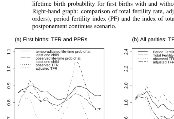
The application of our measures to the description of period fertility patterns is illustrated in Figure 1 that compares our parity progression based measures with the standard and adjusted total fertility rate.
Figure 1: Left-hand graph: comparison of total fertility rate, adjustedT F Rand period lifetime birth probability for first births with and without tempo-adjustment. Right-hand graph: comparison of total fertility rate, adjusted T F R(all birth orders), period fertility index (PF) and the index of total fertility (TF) in the postponement continues scenario.
years
1970 1975 1980 1985 1990 1995 2000
0
.6
0
.7
0
.8
0
.9
1
.0
1
.1
(a) First births: TFR and PPRs
tempo-adjusted life-time prob of at least one child
observed life-time prob of at least one child
observed TFR adjusted TFR
years
1970 1975 1980 1985 1990 1995 2000
1
.4
1
.6
1
.8
2
.0
2
.2
2
.4
(b) All parities: TFR and PF
Period Fertility Index (PF) Total Fertility (TF), continues observed TFR
adjusted TFR
for first births exhibit large fluctuations over time. In comparison to these large fluctu-ations, the period lifetime probability of having at least one child is relatively constant. This is particularly the case after tempo-distortions are removed, and the tempo-adjusted lifetime birth probability neither increases nor decreases as pronouncedly as the standard or adjusted total fertility rate for first births. On the one hand, these different develop-ments are partially due to the fact that changes in the parity distribution of a population subsequent to economic changes or policy interventions can cause fluctuations in period fertility measures that are unrelated to behavioral changes in that specific period. Since Sweden experienced varying socioeconomic conditions and family-policies during the period under investigation (Andersson 1999, 2000; Hoem 2000; Hoem and Hoem 1996; Hoem 1990), the total fertility rate for first births therefore overestimates the volatility of fertility behavior (for related analyses see Ortega and Kohler 2002b; van Imhoff 2001). On the other hand, the differences between the measures in Figure 1(a) are partially due to the fact that neither the standard nor the adjusted total fertility rate for first births rep-resent synthetic cohort measures. Neither measure can thus properly reflect the number of first-births that occur to members of a synthetic cohort based on the level of first-birth fertility in a given period.
Both of the above limitations are avoided using a parity progression based indicator of period fertility, and these measures therefore yield a different—and in our opinion improved—picture of fertility trends for first births. In particular, the tempo-adjusted period lifetime probability of at least one child does not fluctuate substantially during the observation period, and it does not substantially decline in the baby-bust period after 1990.
While the level of first birth fertility has been relatively constant during the baby boom and bust after 1985 in Sweden, this is not the case for the period fertility index (P F) that exhibits substantial fluctuations from 1970 to 1999 (Figure 1b). This index, which equals the complete fertility of women experiencing the tempo-adjusted period childbearing intensities, increases from less than 1.8 in the early 1980s to more than 2.1 in 1990 and subsequently declines again to about 1.7. Since tempo-adjusted lifetime birth probabilities for the first child have remained relatively constant, this analysis implies that the baby boom and bust is primarily due to fluctuations in the parity progression ratios to the second and third child (for related studies, see Andersson 1999, 2000; Hoem 2000; Hoem and Hoem 1996; Hoem 1990; Kohler and Ortega 2002).
differential tempo changes at different parities potentially affect completed fertility. For most periods, the changes in the tempo of fertility tend to be faster for lower parity births and slower for higher parity births. This suggests the presence of a net fertility aging effect so that a continued postponement of fertility tends to reduce the completed fertility. This reduction of total fertility in the postponement continues scenario, as compared to the period fertility index, reaches its highest levels based on the patterns observed around 1980 and in the 1990s. Only in the late 1980s do the differences diminish or even reverse, which is due to the fact that the delayed onset of parenthood is compensated for by suffi-ciently fast tempo changes at second birth. Since a continued delay of childbearing for the foreseeable future seems more likely than an imminent leveling off in the pace of fertil-ity postponement, the period fertilfertil-ity index, which assumes no further postponement, can be regarded as an upper bound for the completed cohort fertility implied by the fertility pattern of a given reference year.
2.3
Continued fertility postponement and cohort fertility
In addition to the measurement of period fertility, our tempo-adjusted parity progression measures are also attractive because they provide a direct application to the projection of cohort fertility. In Figure 2(a), for instance, we consider the cohorts who are 17 and 24 years old in 1999, and we project the proportion of women who will still be childless in the years 2005, 2010,... under the assumption that the 1999 parity-specific fertility levels prevail in the future. These calculations are augmented in Figure 2(b) with the projected level of final childlessness in all cohorts who are still in childbearing ages in 1999.
The full line in these two figures reflects the transition into parenthood that is obtained from the observed childbearing intensities, and these calculations project an ultimate level of childlessness around 23%. However, because the pace of fertility postponement has been quite high during the 1990s in Sweden, this projection is distorted by tempo effects and does not reflect the true cohort experience that is implied by the 1999 level of fertility. The unbiased calculations based on the adjusted childbearing intensities with no further postponement of fertility (dashed lines) project a substantially more rapid transition into parenthood and a substantially lower level of ultimate childlessness of about 15%. Hence, projections based on the observed childbearing intensities, which are tempo-distorted in periods of a fertility postponement, tend to underestimate the fraction of women who are going to experience at least one child given the current level of fertility.
Figure 2: Projection of fertility behavior for cohorts who have not finished childbearing in 1999 based on the level of fertility and postponement pattern observed in 1999 year 0 .1 2 5 0 .2 5 0 0 .5 0 0 1 .0 0 0
2000 2010 2020 2030
(a) Proportion still childless at time t
cohort age 17
cohort age 24
cohort
1955 1965 1975 1985
0 .1 2 0 .1 6 0 .2 0 0 .2 4
(b) Prop. remaining ultimately childless
year
2000 2010 2020 2030
0 .0 0 .5 1 .0 1 .5
(c) Cumulative cohort fertility
cohort age 17 cohort age 24
proj. observed postponement stops postponement continues cohort
1955 1965 1975 1985
1 .5 1 .6 1 .7 1 .8 1 .9 2 .0
reduction due to fertility aging effect
(d) Completed fertility
Notes: The postponement stops (dashed line) and postponement continues (dashed-dotted line) are based on
Table 1: Projected mean age at birth for women in the cohorts born 1982 (age 17 in 1999) and born 1975 (age 24 in 1999)
Cohort age 17 Cohort age 24
in 1999 in 1999
Mean age at first birth
postponement stops scenario 28.34 28.56a
postponement continues scenario 31.56 30.03
calculated from observed data 28.86 28.79
Mean age at second birth
postponement stops scenario 31.05 31.18a
postponement continues scenario 33.76 32.44
calculated from observed data 31.42 30.30
Mean age at birth, all parities
postponement stops scenario 30.01 30.16a
postponement continues scenario 32.57 31.27
calculated from observed data 30.37 30.27
Notes: (a) The difference in the mean age at birth between the 1982 and 1975 cohort in the postponement stops scenario is due to a different age-distribution of births that occur prior to 1999.
effect of a continued postponement on the transition into parenthood is more pronounced in the younger cohort because the postponement continues for a prolonged time until this cohort reaches the primary ages of childbearing.
contin-ued postponement suggests a higher cumulative fertility due to some late first and higher order births. In the cohort that is age 17 in 1999, the postponement continues scenario implies a cumulative fertility level until about 2020 that is substantially below the level suggested by the observed intensities. Due to relatively late childbearing the completed fertility in this cohort will exceed the completed fertility suggested by the observed data, but it will fall substantially short of the level attained by the cohort in the postponement stops scenario. [Note 3] This pattern, which is illustrated for the cohorts who are 17 and 24 years old in 1999, pertains similarly to all cohorts who have not completed fertility as of 1999 (Figure 2d). While the completed fertility of cohorts starts to stabilize at a level of about 1.7 for cohorts who are below age 25–30 in 1999 under the postponement stops scenario, cohort fertility continues to decline in young cohorts if the postponement of fer-tility continues at the pace observed in 1999. These further declines in the postponement continues scenario are due to a net fertility aging effect: the number of higher order births is reduced by an ongoing delay of childbearing because women tend to be ‘at risk’ of second and higher order births only at ages when the probability of experiencing second, third, and fourth births is already quite low. [Note 4]
3
Adjusting Parity Progression Rates for Tempo and
Vari-ance Effects
3.1
A parity and age model of fertility
In this section we begin our formal development of the tempo-adjusted period parity pro-gression measures that we introduced in the previous application to Sweden. As we have pointed out in the previous sections, we develop these measures within a parity and age fertility model that relies on the following assumption:
Assumption 1 Determinants of fertility: Fertility behavior in the population depends only on age, period and parity, and it is independent of the timing of any previous births.
defined as
mj(a, t) = lim
∆t→0Pr(birth of orderj+ 1birth occurs between timet
andt+ ∆t|agea, timet, parityj)/∆t, (1)
where the conditional probability in Eq. (1) is the probability that a woman who is agea
and parityjat timetexperiences a birth of orderj+ 1before timet+ ∆t. [Note 5] Childbearing intensities can be easily converted into parity progression probabilities. For instance, the probability that a woman agexand parity j at timeT experiences at least one additional birth prior to agey, denotedpT
j(x, y), follows from the integration of the childbearing intensitiesmj(a, t)in Eq. (1) along the cohort line in the Lexis diagram as
pT
j(x, y) = 1−exp[− Z y
x
mj(a, T + (a−x))da].
3.2
Tempo distortions in childbearing intensities
In order to analyze tempo distortions in childbearing intensities and derived period par-ity measures, we also need to specify how changes in the tempo and level of fertilpar-ity affect the observed childbearing intensities. For this purpose we utilize the assumption that age, parity and period are the only determinants of fertility (Assumption 1), and we separate the observed childbearing intensities into two factors: first, a level effect,qj(t), that proportionally increases the parity-jchildbearing intensities at all ages; and second, an age-pattern of childbearing intensities,hj(a, t), that evolves over time only due to the postponement of fertility (an analog assumption also underlies the adjustment of the total fertility rate in BF and KP).
Assumption 2 Observed childbearing intensities: The observed intensity schedule for parityjwomen can be decomposed as
mj(a, t) =qj(t)·hj(a, t), (2)
where the termqj(t)is a parity- and period-specific level effect that proportionally in-creases or dein-creases childbearing intensities at all ages, andhj(a, t)is a schedule that determines the age-pattern of the parity-jchildbearing intensities at timet.
over time only due to changes in the timing of fertility at parityj, and it remains constant in periods when there is no postponement or anticipation of fertility at any age. The char-acterization of fertility postponement in our analyses can therefore be based exclusively on the evolution of the age-patternhj(a, t)over time.
In order to provide a benchmark for measuring changes in the timing of fertility, we choose an arbitrary reference yearT. We then specify a hypothetical intensity schedule
φTj(a)that reflects the age-pattern of childbearing intensities that would prevail after the reference yearT in the absence of changes in the tempo of fertility subsequent to the reference yearT:
Assumption 3 Age-pattern of childbearing intensities in absence of tempo changes: If tempo changes are absent at all time periodst ≥ T, the age-pattern of childbearing intensities at parityjdoes not change over time and is given by a standardized schedule
φT
j(a). We assume for simplicity that the integral of this standardized schedule equals unity, i.e., we assume thatRφTj(a)da= 1.
In general, the age-pattern of the intensity scheduleφTj(a)is unknown and needs to be identified and estimated on the basis of the observed age-patternhj(a, t)and its evolu-tion over time. In order to solve this inverse estimaevolu-tion problem, our analysis needs to establish the formal relation between the observed age-pattern of childbearing intensi-ties,hj(a, t), and the hypothetical age-pattern,φTj(a). Once this relation is established within our model, the evolution of observed age-patternhj(a, t)over time can be used to estimate both the extent of tempo changes and the unobserved age-patternφTj(a)in the reference yearT (see Section 3.3).
We introduce the cumulated tempo changeRTj(a, t)as the primary indicator of tempo changes. In a formal sense, the cumulated tempo change is merely a function that allows a transformation of the age-pattern of childbearing intensities over time; its interpretation in terms of fertility postponement will become apparent after our formal definition of fertility postponement below. Specifically, we will show that the cumulative tempo increases with age in periods when births are delayed and decreases with age (and possibly becomes negative) when births are anticipated. Moreover, with the exception of some technical restrictions, the cumulated tempoRT
j(a, t)can be specified in a quite arbitrary manner. Our analyses can therefore capture very general postponement patterns that vary across age, cohort and period. (Note: In the following, we use the notation∆aand∆tto denote partial derivatives of a function with respect to ageaand timet, and we use∆a,tas a shortcut to denote the aging operator(∆a+ ∆t) = ∂a∂ +∂t∂):
Assumption 4 Cumulated tempo change: Denote asRT
and timetfor women of parityj. We require thatRT
j(a, T) = 0and∆aRTj(a, t)|t=T = 0 at all agesa, and additionally we require thata−RT
j(a, t)is increasing ina. [Note 6]
This definition merely specifies the formal properties of the functionRTj(a, t)and does not yet provide an interpretation of cumulated tempo changes in terms of changes in the timing of fertility. In the next step we therefore provide an explicit notion of fertility post-ponement (or delays in childbearing) that is defined and measured in terms of cumulated tempo changesRT
j(a, t)at each parityj. This definition of fertility postponement is based on a comparison of the observed age-pattern of childbearing intensities,hj(a, t), and the age-patternφTj(a)that would prevail att≥T if there were no further postponement of fertility after the reference yearT.
In order to facilitate this comparison, we define two hypothetical probabilities of ex-periencing a birth at parity j. These probabilities are based on the intensity schedules
hj(a, t)andφTj(a)respectively. The specification in terms of these intensity schedules implies that we consider a situation in which there are no changes in the parity-specific level effects; the postponement of fertility is the only process that affects childbearing intensities over time.
First, we consider a woman who is agexand parity j in the referenceT, and who experiences the childbearing intensitieshj(a, t). We then denote asphj,T(x, y0)the prob-ability of a birth of orderj+ 1 to the above woman during the age interval(x, y0], or equivalently, during the time interval(T, T0]whereT0 =T + (y0−x). This probabil-ity follows by integrating the childbearing intensitieshj(a, t)along the cohort line in the Lexis diagram as
ph
j,T(x, y0) = 1−exp[− Z y0
x
hj(a, T + (a−x))da]. (3)
We also define a second probability, denoted aspφj,T(x, y00), that reflects the likelihood of a birth of orderj+ 1to the above woman in the case that there is no further postponement of childbearing after the reference yearT. In this case, the age-pattern of childbearing intensities for all timest ≥T is time-invariant and is given byφTj(a)(see Assumption 3). The probability that the above woman experiences a birth of orderj+ 1during the age interval(x, y00]on the basis of these intensities is obtained by integrating the intensity scheduleφTj(a)as
πφj,T(x, y00) = 1−exp[−
Z y00
x
φTj(a)da]. (4)
Definition 1 Postponement of fertility: A postponement of fertility at parityj implies that for all agesxandy0the probabilitiesphj,T(x, y0)andpφj,T(x, y00)satisfy
ph
j,T(x, y0) =πφj,T(x, y0−RTj(y0, T + (y0−x))), (5)
that is, a postponement of fertility implies thatphj,T(x, y0)is equal topφj,T(x, y00)evaluated aty00=y0−RT
j(y0, T0)withT0=T+ (y0−x).
For illustration, consider a cohort of women who are agexand parityjin the reference yearT, and assume that the ‘risk’ of a birth at parityjis given by the observed age-pattern of childbearing intensitieshj(a, t). In the presence of a postponement, the fraction of women who experience a birth of orderj + 1between age xandy0 (or equivalently, during the time period fromT toT0 = T + (y0 −x)) is given byπh
j,T(x, y0). If there had been no postponement of fertility after the reference yearT, then the same fraction of women would have experienced their births of orderj+ 1between agexandy00 = y0−RT
j(y0, T0), or equivalently during the time interval fromTtoT0−RjT(y0, T0). These age and time intervals are shorter than the corresponding intervals (x, y0] and (T, T0] whenever the cumulative tempoRjT(y0, T0)is positive; that is, whenever there has been a delay of childbearing over time.
The above definition therefore captures the essential element of the postponement of fertility: if there is no change in the level effectqj(t)over time, then delayed childbearing implies that age and time intervals are stretched without affecting the probability of giving birth during these intervals. This condition is reflected in the fact that the birth probabil-ities in the presence and absence of the postponement,πh
j,T(x, y0)andπφj,T(x, y00), are equal. The births at parityjthat occur during the age interval(x, y0]in the presence of a postponement, therefore, would have occurred in the age interval(x, y0−RT
j(y0, T0)]in
the absence of a postponement.
This relation is further illustrated by the Lexis diagrams in Figure 3. In this Lexis diagram, we have chosen the year 1990 as reference periodT for measuring the delay of childbearing. We then consider the births at parityjthat occur during the person-years of exposure that are indicated by the parallelogram ABCD. That is, we consider the births of orderj+ 1that are observed during the period from 1990 to 1991 to the cohort of women who are age 30–31 and parityj in 1990. We assume that the period 1990–91 has been characterized by a constant level effectqj(t)and a delay of childbearing at parityj.
Figure 3: Postponement of fertility in the Lexis diagram
Year
A
g
e
1990 1991 1992
3 0 3 1 3 2
(a) no age-period interactions
cohort born at time 1960 cohort born
at time 1959
A D C B F E
Reference year T = 1990
Year
A
g
e
1990 1991 1992
3 0 3 1 3 2
(b) with age-period interactions
cohort born at time 1960 cohort born
at time 1959
A D C B F E
Reference year T = 1990
Notes: In the left-hand graph the cumulated tempo is a function of only time and not age, while in the right-hand
graph the cumulated tempo depends on both time and age. In the former case, the initial parallelogram ABCD is transformed into another parallelogram AEFD. In the latter case, the transformation is more general and the area AEFD is no longer a parallelogram. Such age-period interactions in the postponement of fertility can lead to changes in the shape of the intensity schedule over time.
The extent of fertility postponement during the period 1990-91 in Figure 3 is reflected by the horizontal and vertical distances between right-side corners of the parallelograms ABCD and AEFD. In addition, this extent is measured by the cumulated tempo at time
t = 1991. For instance, the vertical and horizontal distance between the points B,E equals R1990
j (31,1991), i.e., it is equal to the additional postponement of fertility that has occurred during the period fromt = 1990 tot = 1991 for women who are age 31 in 1991 and were age 30 and parityjin 1990. Similarly, the vertical and horizontal distance between the points C,F is equal toR1990
j (32,1991), which reflects the additional postponement during the period 1990–91 for women who are age 32 in 1991 and were age 31 and parityj in 1990. Births that occur at age 31 and time 1991 (see point B in Figure 3), therefore, would have occurred at time1991−R1990
j (31,1991)and at an age
31−R1990
j (31,1991)if the fertility postponement had been absent (see point E). Since the choice of time periods and cohorts in the above discussion is arbitrary, the same relation holds more generally: births of orderj+ 1that occur at ageaat timetto women who are parityj in the reference year would have occurred at an ageα = a−RT
timeτ =t−RT
j(a, t)in the absence of tempo changes after the reference year, where
RT
j(a, t)reflects the cumulated tempo changes that have occurred between the reference yearT and timet.
The graphs in Figure 3 also reveal the importance of defining the postponement of fertility in the absence of changes in the level effectqj(t). In the case whenqj(t)is held constant over time, the number of births occurring during the person years indicated by ABCD and AEFD are equal: a postponement of fertility at parityjimplies that births at parityj are delayed but not foregone. This property is the essence of our definition of fertility postponement in Eq. (5). In periods when the level effectqj(t)is not constant, however, this equality between the number of births in the presence and absence of a postponement may not hold. In particular, if a delay of childbearing is combined with a declining level effect, the number of births during the person-years ABCD are less than the number during the person-years AEFD. This difference is due to the fact that the postponement of fertility leads to a ‘stretching’ of the person-years AEFD into the larger parallelogram ABCD. This stretching implies that some exposure to births of order
j+ 1is moved to later time periods. During these later time periods, indicated by the area EBCF in Figure 3, the level effectqj(t)is lower than in earlier periods indicated by ABCD. The declining level effect therefore reduces childbearing intensities in addition to the tempo-distortions caused by the delay of childbearing. The number of births occurring during the person-years AEFD and ABCD, therefore, are no longer equal. This implies, for instance, that differences across cohorts in their mean age at first (or second) birth do not necessarily identify the extent of postponement that is relevant for the adjustment of childbearing intensities. In particular, these cohort differences can be due to either trends in the level effect or transformations of the age-pattern of childbearing intensities. Without further assumptions, pure cohort comparisons cannot separate these two aspects. The distinction, however, is essential since only the second aspect, changes in the age-pattern of childbearing intensities, leads to tempo distortions.
On the basis of the above theoretical framework, we can now obtain our first and central result. This result specifies the formal relation between the intensity schedules
Result 1 Observed age-pattern of childbearing intensities: If births are postponed ac-cording to Definition 1, the observed age-pattern of childbearing intensities at parityj are given by
hj(a, t) = (1−∆a,tRTj(a, t))·φTj(a−RjT(a, t)). (6)
Inserting this relation in Eq. (2) then yields the observed childbearing intensities at parity
j,mj(a, t), as
mj(a, t) =qj(t)·(1−∆a,tRTj(a, t))·φTj(a−RTj(a, t)). (7)
The observed parity-jchildbearing intensities at ageaand timettherefore consist of the period-specific level effectqj(t), the Jacobian of the transformation from aandttoα andτ, and finally the standardized scheduleφTj(a−RTj(a, t))evaluated at the age when births would have occurred in the absence of a fertility postponement after the reference yearT.
Unfortunately, however, the decomposition ofmj(a, t)in Result 1 does not yet have an interpretation in terms of ‘adjusted childbearing intensities’ and ‘tempo distortions’ caused by a postponement of fertility. This limitation is overcome in our next step:
Definition 2 Adjusted age-specific childbearing intensities: Denote asm0j(a, t)the ad-justed age-specific childbearing intensities at parityjthat are defined as
m0
j(a, t) =qj(t)·(1−∆aRTj(a, t))·φTj(a−RTj(a, t)). (8)
This definition, in combination with Assumption 4, implies that the adjusted childbearing intensities in reference periodTare equal tom0j(a, T) =qj(T)·φTj(a).
The adjusted childbearing intensities in Eq. (8) are the product of three terms: the period-specific level effectqj(t), a correction term(1−∆aRTj(a, t)), and the fertility rateφTj(α) that would have been observed at ageα=a−R(a, t)at timetif there had been no fertility postponement and no level effects. The correction term is necessary because age-period interactions in the postponement of fertility transform the shape of the intensity schedule. The term(1−∆aRTj(a, t))entails that these transformations in the shape of the schedule in itself do not change the level of the integrated childbearing intensitiesRm0
j(a, t)da.
All changes in this level are attributed to the period-specific level effectsqj(t):
Result 2 Level of fertility: The adjusted childbearing intensities reflect the level effect
qj(t)since Z
m0
In the presence of a fertility postponement, however, the observed childbearing intensities are distorted and they do not reflect the level of fertility at parityjand timet. In particular, the observed childbearing intensities at parityjin the presence of a fertility postponement are only a fraction of the intensities that would be observed at timetin the absence of tempo changes. The observed intensities can thus substantially underestimate the level of fertility at parityjin periods with postponed childbearing:
Result 3 Observed versus adjusted childbearing intensities: The observed childbearing intensitiesmj(a, t)and the adjusted childbearing intensitiesm0j(a, t)are related as
mj(a, t) = (1−rj(a, t))·m0j(a, t), (9)
where the age-and-period specific tempo changerj(a, t)is defined as
rj(a, t) =
∆tRTj(a, t)
1−∆aRTj(a, t)
. (10)
Finally, we point out that the above definition of adjusted childbearing intensitiesm0(a, t), as well as the relations in Results 2–3, are independent of the choice of the reference year
T. The above model can therefore be restated in terms of any other arbitrary yearT0:
Result 4 Choice of reference year: The choice of a reference yearT can be altered to any other reference yearT0by specifying the standardized scheduleφTj0(a)asφTj0(a) =
(1−∆aRjT(a, t)|t=T0)·φTj(a−RjT(a, T0))and redefining the cumulated tempo change
RT0
j (a, t)so that it satisfiesRTj(a, t) = RT
0
j (a, t) +RTj(a−RT
0
(a, t), T0). After this
redefinition of the reference year, all changes in the age-pattern of fertility are then ex-pressed relative to the scheduleφTj0(a), and this schedule is proportional to the adjusted childbearing intensities in the new reference yearT0.
3.3
Measuring and adjusting for tempo changes
Our previous discussion has been very general and allowed for virtually unrestricted post-ponement patterns and cumulated tempo changes. The empirical implementation of the above framework, however, requires specific assumptions about the functional form of the cumulated tempoRTj(a, t). Without such specific assumptions, the standardized sched-uleφTj(a)and the cumulated and age-and-period specific tempo changes,RTj(a, t)and
rj(a, t)are not empirically identified.
Assumption 5 Fertility postponement in terms of mean and variance changes: The age-and-period specific tempo changesrj(a, t)are given by
rj(a, t) =γj(t) +δj(t)[a−(¯aj,T+GTj(t))], (11)
whereγj(t)andδj(t)are smooth functions of time, andGTj(t) = Rt
Tγj(z)dz. We assume thatrj(a, t)<1at all agesaat which the childbearing intensities are positive.
The cumulated tempo changes,RTj(a, t), that correspond to age-and-period specific tempo changerj(a, t)in Eq. (11), is specified by
RTj(a, t) =GTj(t) + [a−(¯aj,T +GTj(t))]·(1−e−D T
j(t)), (12)
whereDT
j(t) =
Rt
Tδj(z)dz.
The reason that motivates the above choice for the age-and-period specific tempo change
rj(a, t)and the cumulated tempoRTj(a, t)is apparent from the following result about the development of the mean age and variance of the adjusted intensity schedule over time:
Result 5 Mean age and variance of adjusted intensity schedule: The mean agea¯j(t) and the variances2j(t)of the adjusted intensity schedulem0j(a, t)are given by
¯
aj(t) = Z
a·m0
j(a, t)da/qj(t) = ¯aj,T+GTj(t)
d¯aj(t)/dt = γj(t)
s2
j(t) =
Z
(a−¯aj(t))2·m0j(a, t)da/qj(t) =s2j,T·e2·D T j(t)
dlogs2j(t)/dt = 2δj(t),
where¯aj,T is the mean age ands2j,T is the variance of the adjusted intensity schedule
m0
j(a, T)at timeT. Moreover, inserting the first expression for¯aj(t)into the specification ofrj(a, t)in Eq. (11) yields a simplified version of the age-and period specific tempo change as
rj(a, t) =γj(t) +δj(t)[a−¯aj(t)]. (13)
The specification of the fertility postponement in Assumption 5 thus leads to particularly simple changes in the mean age and variance of the adjusted intensity schedulem0j(a, t) over time. Specifically, the incremental increase in the mean age at timet is given by
γj(t), and the incremental relative increase in the standard deviation is given byδj(t). Moreover, the termGT
schedule between the reference yearT and some later timet, and the termexp[DT
j(t)]
measures the corresponding relative increase in the standard deviation.
The central insight provided by Result 5 is that the relevant information for the as-sessment of tempo distortions is provided by the moments of the adjusted parity-specific intensity schedules (a similar approach to model tempo changes is also used in Keilman 1994). The above specification in terms of mean changesγj(t)and variance changesδj(t) is therefore particularly convenient for the empirical estimation of tempo changes. More-over, the analog of the BF framework, which implies only shifts in the mean age of the fertility schedules but no changes in the variances, emerges within the above specification whenδj(t)is equal to zero at all times.
4
Parity Progression Measures under Alternative
Post-ponement Scenarios
In this section we utilize tempo-adjusted childbearing intensities defined in Section 3 for two main applications to (a) provide improved synthetic-cohort period measures of fertility and (b) to complete the fertility of cohorts, who are still in childbearing ages, under alternative postponement scenarios that determine future patterns of tempo changes. We begin our formal development with application to cohort completion, and we then present the measurement of period fertility as a special case of cohort completion that considers cohorts at the beginning of childbearing ages under the postponement stops scenario.
4.1
Extrapolation of fertility postponement to future periods
variance changes observed in the reference yearT prevail in the future. The period in-tensity schedule therefore continues to be shifted to later ages during the life-course of the cohorts, and the annual extent of the shift equals the mean and variance change that is observed in the reference yearT. Both scenarios assume that the parity-specific level effects in the reference year,qj(T), continue to prevail in the future for allt≥T.
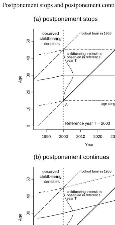
We illustrate these two different postponement scenarios in the Lexis diagrams in Figure 4. In this illustration we choose the year 2000 as the reference year for the calcu-lations. Childbearing intensities are observed prior to this year, and the intensity schedule for the year 2000 is the last available period information. We indicate these childbearing intensities and their age-pattern in a simplified manner through an age range that indicates the minimum, mean and maximum of the intensity schedule. Moreover, the example in Figure 4 assumes that there is a delay of fertility during the years 1980-2000. This post-ponement is reflected through the gradual upward-shift of the age-range of childbearing intensities (for simplicity we assume that there is only a mean change and no variance change). This delay prior to and atT = 2000implies that the observed intensities in the reference year are subject to tempo distortions. These distortions can be eliminated by the adjustment discussed in the previous section. The resulting adjusted intensity schedule for the reference yearT is then the basis for specifying the childbearing intensities that are experienced by the synthetic cohort.
If the postponement stops in the reference yearT, then there are no further changes in the age-pattern of childbearing intensities during the periodst≥T (Figure 4a). Thus, there are no tempo-distortions at timet ≥T, and the period intensity schedules at time
t≥T are equal to the adjusted intensity schedule in the reference year. Consider now the cohort born in 1985 who is age 15 in the year 2000. If the postponement stops scenario prevails, this cohort experiences the childbearing intensities along the diagonal cohort line AB. These childbearing intensities, however, are identical to the adjusted intensities observed in the reference yearT. The analysis along the line AB is therefore equivalent to the analysis of the adjusted intensity schedule at timeT.
Figure 4: Postponement stops and postponement continues scenario in the Lexis diagram
Year
A
g
e
1990 2000 2010 2020 2030 2040
0
1
0
2
0
3
0
4
0
5
0
(a) postponement stops
Reference year T = 2000 observed
childbearing intensities
cohort born in 1955
cohort born in 1985
A
B
age-range of childbearing childbearing intensities
observed in reference year T
Year
A
g
e
1990 2000 2010 2020 2030 2040
0
1
0
2
0
3
0
4
0
5
0
(b) postponement continues
Reference year T = 2000 observed
childbearing intensities
cohort born in 1955
cohort born in 1985
A
B
age-range of childbearing childbearing intensities
after the reference year. The fertility of a cohort that is age 15 in the yearT = 2000, for instance, is obtained by tracing the childbearing intensities along the line AB in Figure 4(b). In contrast to the postponement stops scenario, however, the intensities along the line AB are no longer equal to the adjusted childbearing intensities in the reference year. If postponement continues, the mean age of the period intensity schedule is continuously shifted upwards, and the childbearing intensities that are experienced by the cohort along the line AB are a transformation of the adjusted intensity schedule observed in the year
T = 2000.
Fortunately, we can capture this transformation by extending the formal framework for the postponement of fertility that we have developed in the previous sections. In par-ticular, we can use the observed tempo and variance changes in the reference yearT to specify the cumulated tempo changes for all periodst ≥T. The fertility measures for a cohort therefore follow from the observed childbearing intensities in three conceptually distinct steps: (a) the measurement of and adjustment for tempo-distortions in the ob-served childbearing intensities; (b) the projection of all childbearing intensities fort≥T
based on the adjusted intensity schedule in the reference year and assumptions about the future postponement of fertility; (c) the calculation of completed cohort fertility by inte-grating the intensities obtained in (b) along cohort lines in the Lexis diagram (e.g., along the line AB in Figure 4).
In the following we formalize the above discussion of Figure 4, and we establish the childbearing intensities that would be observed after the reference yearT if the level of the reference year and some arbitrary tempo change and variance change prevails for all times thereafter. These childbearing intensities follow directly from our earlier Result 1 and Definition 2:
Result 6 Extrapolation of fertility postponement to future periods: Denote asmsj(a, t) the parity-jchildbearing intensities that would be observed at ageaand timet ≥ T if (a) the level effectqj(T)observed in the reference yearT prevails for allt ≥ T, and (b) fertility at parityj continues to be postponed with a constant annual mean change
γs
jand variance changeδsjfor allt ≥T. In addition, denote asRsj(a, t)the cumulated tempo and asrs
j(a, t)the age-and-period specific tempo change that are obtained from Eqs. (11–12) usingγj(t) =γsjandδj(t) =δsj for allt≥T. Then
ms
j(a, t) = qj(T)·(1−∆a,tRjs(a, t))·φTj(a−Rsj(a, t)) (14)
= (1−∆a,tRsj(a, t))·mj0(a−Rsj(a, t), T). (15)
The corresponding adjusted intensity schedulems0
j(a, t)for allt≥T is given by
ms0
j(a, t) = (1−rsj(a, t))−1·msj(a, t)
The mean age¯as
j(t)and variances2j,s(t)of the adjusted fertility schedulesmsj0(a, t)at timetare given by¯as
j(t) = ¯aj,T+γsj·(t−T)ands2j,s(t) =s2j,Te2·δ s
j·(t−T), wherea¯j,T ands2
j,T are the mean age and variance of the adjusted intensity schedulem0j(a, T)in the reference yearT. Moreover, the integrals of the observed and adjusted childbearing intensities for allt ≥ T are constant over time and equal respectivelyR ms
j(a, t)da=
(1−γs
j)·qj(T)and
R
ms0
j(a, t)da=qj(T).
The above result therefore allows us to calculate hypothetical intensity schedules that would be observed at some timet ≥T if (a) the level effect observed in the reference yearT at parityj prevails in the future, and if (b) fertility is subject to a postponement pattern with a constant annual mean changeγsj and variance changeδsj for allt ≥ T. The mean age of the adjusted intensity schedule at parityj then increases annually by
γs
jyears, and the standard deviation grows exponentially at an annual rate ofδsj. [Note 7] Moreover, the integral of the adjusted childbearing intensities remains constant for all
t≥Tand equals the level effectqj(T)in the reference yearT.
We subsequently use the phrase that calculations pertain to the ‘period-T cohort of agex’ in order to describe the following assumption about the fertility experience of the cohort for which parity progression measures are calculated:
Assumption 6 Parity progression measures for the period-T cohort of age x: In our calculations of parity progression measures we assume a cohort, denoted period-T cohort of agex, who (a) is agexin the reference yearT and (b) experiences the childbearing intensities that are obtained by extrapolating the level of fertility and the pace of fertility postponement observed in the reference yearTto all timest≥T. That is, we assume that women in the period-T cohort of agexare subject to the childbearing intensitiesms
j(a, t)
defined in Eq. (14) when they attain ageaat timet=T+ (a−x).
We use the term ‘period-T cohort of agexand parityj’ if we additionally condition on parity and consider women who are at exact parityjin the reference yearT.
The maximum feasible age at childbearing (‘biological limit’) is given byω. We as-sume that this age does not imply a restriction for the postponement of fertility in our analyses, i.e., we assume that the childbearing intensities defined in Eq. (14) satisfy
ms
j(a, T +a−x) = 0for alla≥ω. [Note 8]
Our two basic approaches to determine the pace of fertility postponement in the synthetic cohort are specified as follows: (a) ‘extrapolate’ the postponement pattern observed at timeT, i.e., assume that the mean changeγsjand variance changeδsjduring the life-course of the cohort equal the values ofγj(T)andδj(T)observed in the reference yearT for all paritiesj; (b) assume that there are no further postponements of fertility subsequent to timeT, i.e., assume thatγs
postponement continues and the latter the postponement stops scenario. [Note 9] In our subsequent notation, we indicate the postponement stops scenario as ‘γsj = 0, δsj = 0’ and the postponement continues scenario as ‘γsj = γj(T), δsj =δj(T)’. For simplicity, we often drop the subscriptjfor fertility measures that combine several birth parities, and we use ‘γs, δs’ as a shorthand notation for ‘γs0, γs1, . . . , δs0, δs2, . . .’.
4.2
Conditional parity progression probabilities
The primary building block for deriving the parity progression ratios for the period-T cohort of agexis the conditional parity progression probability that is calculated condi-tionally on a postponement scenario described byγsjandδsj:
Result 7 Conditional parity progression probability: Consider a woman in the period-T cohort of agexand parityj. This woman is exposed to a birth of orderj+ 1from agex and timeTonwards. Denote aspTj(x, y|γs, δs)the probability that this woman attains a parity of at leastj+ 1at agey(withy≥x) by having at least one additional child prior to agey.
Integrating the childbearing intensitiesmsj(a, t)experienced by the period-T cohort of agex(see Eq. 14) yields
pTj(x, y|γsj, δsj) = 1−exp ·
−
Z y
x
msj(a, T +a−x)da ¸
= 1−exp
"
−
Z y−Rs
j(y,T+(y−x))
x
m0j(a, T)da #
. (17)
In the specific casey=ω, the conditional lifetime parity progression probabilitypT
j(x, ω|
γs
j, δsj)reflects the probability that a woman in the period-T cohort of agexand parityj has at least one additional child and progresses to parityj+ 1or higher. This probability is given by the integral of the adjusted parity-j age-specific childbearing intensities at timeTfrom agexonwards,
pT
j(x, ω|γsj, δsj) = 1−exp ·
−
Z ∞
x
m0
j(a, T)da
¸
,
and is thus independent of the assumption aboutγsjandδsj.
assumptions about future mean- and variance changes at parityj affect only the upper limit of the integral in Eq. (17). The conditional parity progression probability—as well as all subsequent parity progression measures—can therefore be obtained without ever calculating the childbearing intensitiesmsj(a, t)(see Eq. 14) that are experienced by the period-T cohort of agex. This feature makes the calculation of different postponement scenarios particularly simple. All postponement scenarios are obtained by integrating the adjusted intensity schedule in the reference yearT, and the assumptions about the future postponement of fertility only need to be considered in the upper limit of the integral.
The above result has several interesting implications. First, the exponent of the in-tegral of the adjusted childbearing intensities yields a proper assessment of conditional parity progression probabilities in cohorts. Second, in order to estimatepT
j(x, ω|γsj, δsj),
i.e., the probability that a woman who is agexand parityjat timeThas another child, it is sufficient to know the adjusted age-specific childbearing intensitiesm0
j(a, T). No further assumptions about the future path of fertility postponement are necessary. Third, since in periods of fertility postponementm0
j(a, t)exceeds the observed intensitiesmj(a, t), a calculation of the conditional parity progression probabilitypT
j(x, y|γsj, δsj)on the ba-sis of the observed childbearing intensities would underestimate the probability to have another child:
Result 8 Distortion of conditional parity progression probability due to tempo changes: The calculation of the conditional parity progression probabilitypT
j(x, ω|γsj, δsj)in Eq. (17) based on the observed instead of the adjusted childbearing intensities is distorted. In the specific case when δj(T) = 0 and δsj = 0, i.e., in the absence of variance changes for parity j, the calculation based the observed intensities yields 1 −(1−
pT
j(x, y|γsj, δsj))1−γj(T). This probability is smaller than the correct value pTj(x, y|
γs
j, δsj)obtained from the adjusted childbearing intensities whenever the mean change
γj(T)at timeT is positive. Moreover, the calculations based on the observed intensities always underestimates the correct value of the lifetime birth probability,pTj(x, ω|γsj, δsj), wheneverγj(T)>0andδj(T)≥0.
The failure to account for tempo distortions therefore leads to erroneous inferences of period parity progression probabilities and related measures.