SiSeRHMap v1.0: a simulator for mapped seismic response using a hybrid model

(1)

www.geosci-model-dev.net/9/1567/2016/ doi:10.5194/gmd-9-1567-2016

SiSeRHMap v1.0: a simulator for mapped seismic response

using a hybrid model

Gerardo Grelle1, Laura Bonito2, Alessandro Lampasi3, Paola Revellino2, Luigi Guerriero2, Giuseppe Sappa1, and Francesco Maria Guadagno2

1_{Department of Civil and Environmental Engineering, University of Rome “La Sapienza” via Eudossiana 18,} 00184, Rome, Italy

2_{Department of Sciences and Technologies, University of Sannio, via Dei Mulini 59/A, 82100, Benevento, Italy} 3_{ENEA Frascati Research Center, Via Enrico Fermi 45, 00044 Frascati, Rome, Italy}

Correspondence to: Gerardo Grelle ([email protected], [email protected])

Received: 19 March 2015 – Published in Geosci. Model Dev. Discuss.: 17 June 2015 Revised: 25 March 2016 – Accepted: 8 April 2016 – Published: 26 April 2016

Abstract. The SiSeRHMap (simulator for mapped seismic response using a hybrid model) is a computerized method-ology capable of elaborating prediction maps of seismic re-sponse in terms of acceleration spectra. It was realized on the basis of a hybrid model which combines different ap-proaches and models in a new and non-conventional way. These approaches and models are organized in a code ar-chitecture composed of five interdependent modules. A GIS (geographic information system) cubic model (GCM), which is a layered computational structure based on the concept of lithodynamic units and zones, aims at reproducing a param-eterized layered subsoil model. A meta-modelling process confers a hybrid nature to the methodology. In this process, the one-dimensional (1-D) linear equivalent analysis pro-duces acceleration response spectra for a specified number of site profiles using one or more input motions. The shear wave velocity–thickness profiles, defined as trainers, are randomly selected in each zone. Subsequently, a numerical adaptive simulation model (Emul-spectra) is optimized on the above trainer acceleration response spectra by means of a dedicated evolutionary algorithm (EA) and the Levenberg–Marquardt algorithm (LMA) as the final optimizer. In the final step, the GCM maps executor module produces a serial map set of a stratigraphic seismic response at different periods, grid solv-ing the calibrated Emul-spectra model. In addition, the spec-tra topographic amplification is also computed by means of a 3-D validated numerical prediction model. This model is built to match the results of the numerical simulations re-lated to isolate reliefs using GIS morphometric data. In this

way, different sets of seismic response maps are developed on which maps of design acceleration response spectra are also defined by means of an enveloping technique.

1 Introduction

In the scientific community, it is well known that lithologic stratigraphy as well as topographic features are capable of considerably amplifying the local destructive action of an earthquake (Del Prete et al., 1998; Athanasopoulos et al., 1999). Thus, in prone areas, seismic microzonation studies assume an important role in urban planning and seismic risk management (Lachet et al., 1996; Bianchi Fasani et al., 2008; Compagnoni et al., 2011; Milana et al., 2011; Grasso and Maugeri, 2012; Moscatelli et al., 2014). As a consequence, methods for high levels of seismic microzonation (mapped seismic response studies) aim at providing quantitative data for use in building design (Borcherdt, 1994; Todd and Har-ris, 1995; Bostenaru Dan, 2005; Kokošin and Gosar, 2013). Many building codes, such as Euro Code 8 and FEMA 356 (2000), require seismic design actions defined by simplified elastic acceleration spectra deriving from local base seismic hazard (as reference natural or virtual stiff rock site which are defined in term of horizontal acceleration probability of exceedance in specified time interval) and site amplification effects.

(2)

1568 G. Grelle et al.: SiSeRHMap v1.0 data management and spatial distribution in terms of input

and output/outcomes, are also required. Therefore, the ge-ographic information systems (GIS) contribute the most to maximizing the available data, in the assessment or esti-mation of ground-motion amplification (Kolat et al., 2006; Ganapathy, 2011; Hashemi and Alesheikh, 2012; Turk et al., 2012; Hassanzadeh et al., 2013) and seismic-induced effects (Grelle et al., 2011; Grelle and Guadagno, 2013).

In this aforementioned context, SiSeRHMap (simulator for mapped seismic response using a hybrid model) provides synthetic multi-map data regarding a complex phenomenon, such as seismic site response, on the basis of a new hybrid methodology in which a meta-modelling process is the core feature. In recent years, the use of meta-models in many en-gineering and environmental science fields (Lampasi et al., 2006; Yazdi and Neyshabouri, 2014; Wang et al., 2014; Hong et al., 2014), together with GIS supported analysis (Reed et al., 2012; Fan et al., 2015; Soares et al., 2014), has produced good performances, providing fast versatility and rapid up-dating.

By nature hybrid systems based on meta-models include intrinsic uncertainty in their predictions. This is due to the use of non-physical adaptive models trained on simplified physical models. On the other hand, these systems permit an efficient analysis in terms of expected performance. Es-sentially, a meta-model permits a quick replication of the so-lutions in a limited context of randomness. In this way the proposed model is very suitable for a continual easy modular update that decreases the epistemic uncertainty, over time, in the assessment of the effects of natural complex phenomena, such as seismic response, on a real natural system. There-fore, SiSeRHMap is formulated on the concept of “perfor-mance”, regarding (i) prediction, (ii) easy and low compu-tational time, (iii) upgrading, and (iv) output accessibility (GIS-georeferenced data), with respect to the real effect. For these reasons, SiSeRHMap aims at giving a substantial con-tribution to common practices. Contextualized for a practical application in site seismic response studies, limits of usual practice may be currently summarized as (i) a partial contri-bution of the microzonation study with regards to providing appropriate quantitative parameters for seismic engineering practice; (ii) an inadequate use of some simplified ampli-fied design spectra defined by means of some large ranges of

VSthat refer to 30 m or to the deep bedrock; (iii) an unsuit-able use of the point-data spatial interpolation for the mapped seismic response values.

Considering the aforementioned critical issues, in areas with a not very high geological complexity, the proposed methodology can present a high computational efficiency in comparison to expensive rigorous physically based models; this efficiency multiplies when a probability multi-input mo-tion analysis is performed. Therefore, the map-sets of seis-mic response provided by SiSeRHMap are the result of an advantageous compromise between intrinsic and epistemic uncertainties and the accuracy and robustness required. This

last aspect reflects the aptitude of the proposed methodology, which is suitable for analysis of urban areas or relatively vast areas. In general the level of accuracy of the SiSeRHMap re-sponse increases with the number and quality of the surveys; however, it is suitable to be used in areas with common and non-strategic facilities (e.g. nuclear plants); for strategic fa-cilities, a detailed analysis may be required due to the fact that the use of a meta-model might not ensure the level of accuracy required.

1.1 Code design and aims

SiSeRHMap is a computer program methodology aimed at the mapped simulator for mapped seismic response using a hybrid model. The hybrid model consists of a complex computational system composed of a GIS frame model, an-alytical models (physically based) and meta-modelling pro-cedures. SiSeRHMap is capable of developing map sets of seismic response taking into account the combined effects of plane-parallel stratigraphy and real topographic features. It is composed of five progressive interdepending Python com-pute modules, each of which necessitates external input data. The input data and data set are inserted or linked into a textual user interface (TUI) which writes the file “Instruc-tion.txt” that the Python modules read in running.

The modules and their computational functions are as fol-lows:

– mod.1: lithodynamic units parameterization; – mod.2: GIS cubic model frame;

– mod.3: stratigraphic response; – mod.4: training “spectra”; – mod.5: GCM maps executor. 1.2 Background

In mapped seismic response studies carried out using analyt-ical methods for assessing or estimating stratigraphic seis-mic site responses, GIS provide the spatial distribution of parameters, which characterize the seismic motion (Jimenez et al., 2000; Sokolov and Chernov, 2001; Nath, 2004; Kien-zle et al., 2006). Based on a multi-variate regression analysis of common recurrent regional data settings regarding simple sequences, procedures for calculating seismic soil response have also been introduced (Rodríguez-Marek et al., 2001; Pa-padimitriou et al., 2008).

(3)

stress–strain behaviour. The zone is defined by a specific combination, in sequence, of lithodynamic units. The hy-brid model computes the mapping of seismic response us-ing an adaptive model, which is trained on one-dimensional (1-D) seismic response target cases calculated from some shear wave velocity–thickness sequences. These latter are uniformly randomly selected in coherence with general litho-dynamic layered models assumed for the study area. In this way, the trained adaptive model, conceptually defined as a meta-model (replacement model), is used in the spatial pre-dictive analysis, which aims at developing seismic response maps by means of its meta-model solving in the GCM.

Topographic amplification is a more relevant frequency dependent effect in zones characterized by hill and moun-tain features (Çelebi, 1987; Kawase and Aki, 1990; Assimaki et al., 2005; Del Gaudio and Wasowski, 2007; Hough et al., 2010; Massa et al., 2010; Pischiutta et al., 2010). 2-D and 3-D simulation analytical approaches on different relief shapes, as well as different incident seismic wave motions, have been introduced (Sánchez-Sesma, 1983; Geli et al., 1988; Ashford et al., 1997; Durand et al., 1999; Maufroy et al., 2012, 2015). Geli et al. (1988) used numerical methods for assessing the topographic amplification factor,AT, of the vertical incident of horizontal shear waves (SH) on 2-D isolated reliefs con-stituted by uniform material and different layering structures. Their results highlighted that the frequency-dependent am-plification factors change considerably along the topographic surface, showing a greater amplification at the ridge, reach-ing values over 2.00 in some cases. Ashford et al. (1997) quantified the theoretical effect of the horizontal and verti-cal seismic response at a ridge of monoclinal slopes, which is half-space extensive, by taking into consideration verti-cal incident SH waves. The analytiverti-cal model assumes that the slopes are constituted by uniform viscoelastic material (damping=1 %). The topographic amplifications factor in relation to the dimensionless frequency H /λ, where H is the relief height and λis wavelength, confirms that greater amplification occurs atH /λ=0.2. This corresponds to the topographic fundamental period TfT=5H /VS of the relief. Similar values of resonance were found by Paolucci (2002); however, slightly lower values were also shown for high fre-quencies. In addition, in relation to the slope angle i, the

AT H /λ-depending curves decrease showing greater val-ues fori=90◦(AT≈1.5), while they are lower fori≤30◦ (AT<1.10) and negligible fori=15◦. Similar values were obtained for the same relief model by Nguyen et al. (2013).

In natural complex topographic zones, Maufroy et al. (2012) used a 3-D numerical simulation code in order to investigate topographic effects, in some assigned points, as-suming a multi-isotropic source of seismic waves propagat-ing in a complex 3-D media with a realistic surface topog-raphy. Their results showed topographic amplification fac-tors up to 3.6 with a typical value range of 1.5–2.5 at the crests. However, the 3-D topographic amplification seems to be the combined result of lithological and geometric factors

in which the pure topographic effect is difficult to fully quan-tify in numerous cases (Gallipoli et al., 2013). In addition, in some cases, recorded ground motions show a directional-ity in the resonance, (Bouchon et al., 1996; Spudich et al., 1996) encountering amplification values greater than the re-sults formulated by the 2-D and 3-D numerical simulation models (Lovati et al., 2011). Furthermore, most comparison studies refer to noise or weak aftershock motions, and thus do not take into account or only slightly take into account the non-linear effect of system ridge lithology (Gutierrez and Singh, 1992). On the other hand, the aforementioned studies have increased awareness in relation to the necessity to assess or predict topographic effect as a frequency depending vari-able and in an adequate way, in contrast with the simplistic models of the building codes. These models, in fact, provide the use of constant amplitudes in the entire spectrum, show-ing conditions of under-evaluation in several spectral ranges (Gallipoli et al., 2013; Barani et al., 2014).

1.3 Application scenarios

SiSeRHMap was applied to a synthetic recurrent scenario (SRS), a fictitious area of 5 km2(2.5 km×2.0 km), which is a synthetic reproduction of a common hilly scenario char-acterized by rigid/quasi-rigid reliefs and a valley with soft lithologic units covering the bedrock: the term “rigid/quasi-rigid” refers to the shear wave velocity values of the material constituting the relief.

The choice for using a SRS was based on the following reasons: (i) the possibility to simulate a vast number of se-quences with different layer combinations in order to demon-strate the complete computational ability of SiSeRHMap; (ii) the possibility to introduce different comparison scenar-ios, including also real scenarscenar-ios, in the analysis, as shown in the topography amplification section (Sect. 4.2). The recog-nizing, consultation, and interpretation of pre-existing data is a fundamental process in the definition of lithodynamic units and their spatial distribution (lithodynamic model). However, this preliminary process does not affect the performance of the code (therefore the methodology) but it affects the coher-ence of the results with the analysed area.

(4)

1570 G. Grelle et al.: SiSeRHMap v1.0

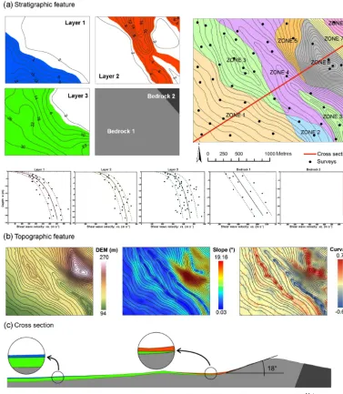
Figure 1. Synthetic recurrent scenario (SRS). (a) On the left: the maps with a resolution of 2.00 m regarding the covered layers and bedrock

layers; for each covered layer, the iso-thicknesses of the relative lithodynamic unit, resulting from the interpolation of the hypothesized field survey is reported (black point in lithodynamic units map); the coloured polygon is the correct extension of the unit corresponding to an iso-thickness of 3.00 m (Sect. 2.2); on the right: the zones characterizing the synthetic recurrent scenario (SRS) are shown; (b) topographic features in terms of the DEM (digital elevation model), slope, and curvature maps with a resolution of 30 m.; (c) cross section with zoom of the covered lithodynamic units sequence.

The stratigraphic feature of the SRS (Fig. 1a) identified three cover lithodynamic units and two bedrock, respectively, rigid and non-rigid conditions (hard rock and soft rock); with regards to the proposed methodology, the meaning of this wording will be better explained in Sect. 2. The combina-tion of these units determines the constitucombina-tion of eight zones. The number and spatial distribution of the survey points are assumed coherent in the parametric characterization, and in the geometric features of the lithodynamic units, in reference to the simple subsoil setting of the SRS. For example, if in

(5)

pre-diction, which is based on using and/or interpreting direct or indirect survey data, the number, typology, and spatial distri-bution of data must be taken into account in relation to the geological complexity of the real area and the required relia-bility accuracy degree desired (Cardarelli et al., 2008).

The topographic feature (Fig. 1b) is characterized by a flat valley zone and a moderate high isolate relief with a slope angle of approximately 15–20◦ and values of curva-ture, at the ridge, of approximately 0.5. The resolution of the stratigraphic grid-data files and topographic grid data is different, in order to respect the resolution expected by SiS-eRHMap (see Sect. 4.2). The georeferenced coordinates of the input/output grid-data files locate the SRS in southern Italy in an unreal way.

2 GIS cubic model: mod1 and mod2

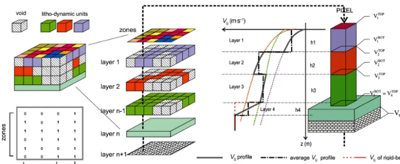
The GCM (Fig. 2) is a discretized and parameterized rep-resentation of an underground half-space that is capable of performing an overlay computation of geo-referenced grid data generated by common geographic information systems platforms. This model intervenes in the SiSeRHMap in two different and non-subsequent phases. In the first phase, the model parameterizes the lithodynamic units. In the second phase, the model produces seismic response maps. The GCM structure (Grelle et al., 2014) is based on a binary template matrix in which the rows (records) and columns (fields) rep-resent, respectively, the zones and layers.

In each zone, the presence or absence of the lithodynamic unit is defined in a binary way with attributes, respectively, value1 and 0. Hence, the layer, the computational entity al-ways present in the matrix, assumes a physical entity inside it where the lithodynamic unit formalizes its presence assum-ing value 1. The presence/absence of lithodynamic units is an exclusive propriety attributed to the covered layers. In con-trast, the bedrock layer is always present at the base of the sequence. In this way, for an-layer sequence, the maximum number of possible zones is 2n−1. The bedrock is the litho-dynamic unit, which is always present at the bottom of the sequence at thenth layers and it can be defined as rigid or non-rigid bedrock, depending on whether the shear wave ve-locity is equal or greater to a prefixed threshold value,VSrig;

in general terms, the aforementioned bedrock typology can represent lithodynamic units composed of massive rock or weak rock. Accordingly, the term “rigid” qualifies a rela-tive and not absolute stiffness (e.g. infinite stiffness) of the bedrock. Therefore, the condition that the non-rigid bedrock must reach the VSrig value, with depth passing thus to the

rigid condition, is imposed; in this way a new lithodynamic unit up to the rigid bedrock is generated by the model; In SiSeRHMap, it is possible to consider the existence of two different bedrock typologies, thereby doubling the number of possible zones (2×2n−1)when this occurs.

2.1 Initial input data

In the GCM, the number of layers, and consequently the spa-tial extension of the lithodynamic units, are jointly defined by preparatory studies, as is the standard procedure in high levels of seismic microzonation. These studies are based on a preliminary collection of field surveys and pre-existing stud-ies and data sets. Subsequently, an accurate interpretation of geological, geotechnical, and geophysical data permits the definition of both the typology and characterization (param-eterization), as well as the spatial distribution, of the lithody-namic units.

The main focus in the parameterization of lithodynamic units is their spatial identification; this latter can be per-formed taking into account the lithology and their shear wave velocity–depth value distributions. In this way, a layer is as-sociated with each lithodynamic unit in the GCM and it is de-fined by a log-linear or linear depending curve,VS–z, which is identified by the intercept-velocityVS0i and angular

coef-ficient αi. In some cases, this identification can show how the geophysical and geotechnical proprieties of soils can be decisive in the building of a GCM model. Therefore, the equations associated with theVS–zlithodynamic unit distri-butions are

i. log-linear function forith covered layer,

VSi(z)=VS0_i+αilog(1+z), (1)

ii. linear function for non-rigid bedrock,nth layer

VSn(z)=VS0n+αnz; whereVS0n< VSRB, (2)

iii. constant value of shear wave velocity for rigid bedrock

VSn(z)=VS0n; whereVS0n≥VSRB. (3)

(6)

Figure 2. Subsoil half-space modelling by the GIS cubic model (GCM) and binary template matrix (e.g. referred to four layers, three covered

layers, and one non-rigid bedrock) and 1-D layeredVS–hprofile deriving from the GCM computational analysis (figure from Grelle et al.,

2014).

Figure 3. Example of the thicknesses cutting performed by mod2

of the SiSeRHMap.

correlation is observed for high N60 values. It is worth not-ing that the relation ofVSincreasing with N60-SPT values is independent from the depth. Therefore, for the material con-stituting the non-rigid bedrock, theVS-depth linear increas-ing relation can be considered valid both in the buried and outcropping condition.

The curve fitting, and therefore the calibration of the pa-rameters VS0i andαi, are obtained by means of the

least-squares regression method (data and graphics in Supplement folder: OUTPUT\mod1_VsZ).

2.2 GCM frame

Input grid data files containing the thickness spatial distri-bution of the lithodynamic units are necessary to instruct mod.2. These files are obtained via the common analysis that led to the definition of the lithodynamic units and zones. In fact, taking into consideration that the limit of a zone is also

the extension line of at least one of the lithodynamic units, polyline features should define the minimum thickness as well as the borderline in the GIS pre-processing . In order to avoid computational bugs, the minimal thickness,h(min), of the lithodynamic units must not be zero. More specifically, this must correspond to the depth of the output of the de-sired seismic response,z(out). Figure 3 shows how the lithol-ogy with a thickness of less thanh(min) did not identify the lithodynamic unit’s presence; therefore, its spatial size must be preliminarily attributed to the nearest lithodynamic unit (above or below the non-identified lithodynamic unit); in 1-D seismic response analysis (mod.3 Sect. 3.1), theh(min) is returned in the corresponding outcropping lithodynamic unit for the computation.

In summary, the georeferenced input raster data (ASCII grid file format) are

– Layer_1.txt, Layer_2.txt, . . . Layer_n-1.txt: extension of the covered layers in terms of one and zero values; – Bedrock_1.txt, Bedrock_2.txt (if this latter is present):

extension of one or two bedrock typologies in terms of one and zero values;

– Zones.txt: extension of zones that are identified from a relative integer number;

– H_layer1.txt, H_layer_2.txt, . . . H_layer_n-1.txt: litho-dynamic unit thicknesses obtained using appropriate GIS spatial interpolation techniques. For an adequate computational time, the grid-data resolution may be de-termined as follows:

top resolution unit (m)≈integer 

 s

surface(m2)

106 

(7)

SiSeRHMap generates new “H_layer(i)_cor.txt” files in which the thicknesses less than h(min) are reported as zero. In this way, the extension of the lithodynamic units is defined in relation to the map extension of the zones. (Some grid input files are reported in the Supplement folder: INPUT\GIS_in.)

2.3 GCM forVS–htrainer models

Once the VS–zcurves have been obtained, and the binary template matrix has been inserted and the georeferenced grid files loaded, the GCM is thus structured and parameterized. In this phase, the GCM could start the mapped parameteriza-tion of the shear wave velocity for each layer as reported in Grelle et al. (2014). However, in SiSeRHMap this computa-tional process is performed in a subsequent second phase of the GCM (mod.5). In this first phase, the GCM gives data re-garding the thicknesses range of the lithodynamic units in the zones to obtain the appropriate VS–h trainer models repro-ducing the 1-D subsoil models as selected in a randomly uni-form way in the GCM. Therefore, the nature of the method-ology requires that the equations, which characterize and pa-rameterize the GCM, are equal to those that will be used in the generation of theVS–htrainer models; thus, these equa-tions will be subsequently circumstantiated at a generic (x, y) geographic point, in the second phase of the GCM (GCM maps executor).

The VS–h trainer models (Fig. 4) are defined by the subsequent equations (5 to 10) using the thickness values extracted, from the uniformly random distribution (Monte Carlo technique), within the maximum and minimum inter-vals found for each lithodynamic unit in each zone. The num-ber of the models generated is freely chosen but it should be assumed taking into account thickness variability and the number of the lithodynamic units present in the zones (the default value is 10).

Therefore, once the GCM has been structured according to a (m×n) binary template matrix and theqnumber of theVS– htrainer models has been established, mod.2 of SiSeRHMap generates the VS–h trainer models. In this way, the param-eterization of an ith layer (i in [1, n]) in ajth zone (j in

[1, m]) for akthVS–htrainer model (kin [1, q]) are defined by the following points.

i. The shear-wave velocity at the top and bottom of each

n−1 cover layer is obtained using the parameterized log-linear functions; in relation to the combining of the layers position, the inversion of shear rigidity is also possible.

VSi(j,k)top =VS0i+αi (

log "

1+ n−1 X

i=1

hi−1(j,k) !#)

(5)

VSi(j,k)bot =VS0i+αi (

log "

1+ n−1 X

i=1 hi(j,k)

!#) (6)

ii. With regards to the rigid bedrock,VSrig, it is defined in

relation to an established threshold of the shear wave ve-locity (e.g.VSrig≥800 m s

−1_{, EC8 prEN1998). In this} way, the rigid bedrock is defined by a unique value of the shear-wave velocity VSRB with the condition that

VSRB≥VSrig.

In contrast, when the bedrock is non-rigid (geological bedrock), the GCM automatically generates a new layer with a thickness ofhn(x,y)and it assumes thenth posi-tion while the rigid bedrock layer shifts to the (n+1)th position. The latter layer has a lithodynamic nature sim-ilar to non-rigid bedrock but its depth confers to it the characteristics of rigid bedrock with a shear wave ve-locity equal toVSRB. This condition is defined by the

following equation:

VSn(j,k)bot =VSRB (7)

thus it results that

hn(j,k)=

VSRB−VSn(j,k)top

αn

, (8)

where

VSn(j,k)top =max

VSn−1(j,k)_bop;VS0n,

(9)

αn is the gradient, and the VS0n is the intercept value

relating to theVS-depth regression linear curve of the non-rigid bedrock (Eq. 2). In Eq. (8), when the max value isVSn−_1Bot, the possible increment of rigidity due

to the lithostatic load of the upper cover layers is taken into account; this case is manifested when the non-rigid bedrock shows relatively low values of the shear wave velocity in the spatial statistical uncertainty of theVS, z values. In contrast, when the max value isVS0n, this

in-dicates that the non-rigid bedrock is near to the rigid condition and therefore it shows relatively high values of the shear wave velocity in theVS–zdispersion curve. iii. The average shear-wave velocity of each lithodynamic

unit is

¯ VSi(j,k)=

1 2

VSi(j,k)top+VSi(j,k)_bot

. (10)

iv. The fundamental vibration period computed consider-ing the average shear wave velocity obtained usconsider-ing the average travel time:

Tf(j,k)=

4 n P

i=1 hi(j,k)

n P

i=1 hi(j,k)/

n P

i=1

hi(j,k)/V¯Si(j,k)

. (11)

(8)

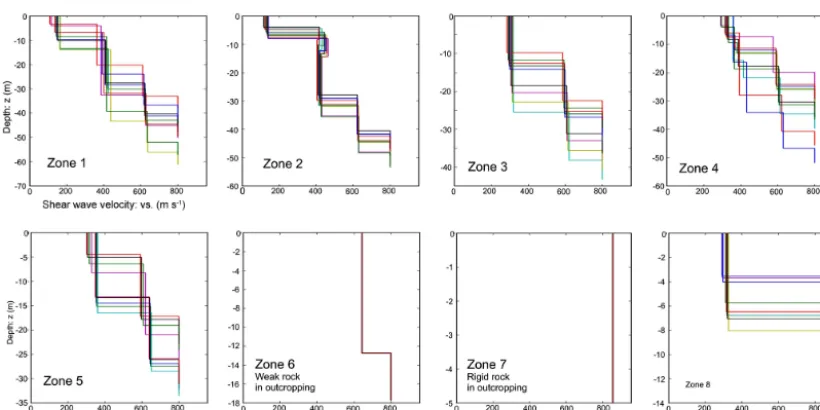
Figure 4.VS–htrainer models: there are 10 trainer models theoretically encountered in each of the eight zones, which are presented in the

SRS (Fig. 1a).

3 Meta-modelling: mod3 and mod4

The meta-model process is the core of SiSeRHMap. This process is composed of a semi-automated computation of the stratigraphic seismic responses of the VS–h trainer models selected. Subsequently, a new robust and performing predic-tion model “Emul-spectra” is trained on the spectral shape of these responses in order to emulate the stratigraphic seismic response in the succeeding GCM maps executor (mod.5). 3.1 Stratigraphic seismic response

The stratigraphic acceleration response spectra is performed in SiSeRHMap by mod.3: stratigraphic response. Here, the dynamic site response is computed in a similar way to other computer program/codes: SHAKE (Schnabel et al., 1972; Idriss and Sun, 1992; Ordónez, 2009), EERA (Bardet et al., 2000), and STRATA (Kottke and Rathje, 2008, 2010). The module computes the dynamic acceleration response that refers to a 1-D soil column using a planar vertical wave propagation model, which takes into consideration an equiv-alent shear-strain-dependent dynamic response of the soil se-quence. This method is commonly referred to as the vis-coelastic equivalent linear analysis, in terms of total stress, taking into consideration a linear elastic bedrock. A horizon-tal polarized propagation of the shear waves through a site with infinite horizontal layers is assumed (Appendix A).

Despite the same computational performance of similar software (Fig. 5), mod.3 is dedicated to processing uploaded data from previous modules and subsequently returns data that are used in the next computational module (mod.4). Specifically, the Stratigraphic Seismic Response module per-forms an automatic computation of all the selected VS–h

trainer models. The natural unit weight,ρ, associated with each layering profile is empirically estimated in relation to the shear wave velocity. In this way, taking into account the low influence of this variable on the shear modulus due to its limited variation, the natural unit weight can be defined (Keçeli, 2012) as

ρ=4.4V_S0.25, (12)

whereρis expressed in kN m−3.

The input motion is considered on the outcropping to the rigid rock. Therefore, it is always deconvoluted within the sequence on the rigid bedrock (layernorn+1), when the covered layers are present in the zone. The output response (Fig. 6) is provided at the outcropping of the surface detected by the assignedzoutdepth; this surface is within the upper layer.

For each covered lithodynamic unit, as well as the non-rigid bedrock, the initial damping ratio, such as the strain-dependent values of the normalized shear module and the damping ratio, must be inserted. From these latter values, the damping ratio and shear modulus degradation curves are obtained using the regression analysis in theG(γ )/G0 and D(γ )ratio curves fitting, which was introduced by Yokota et al. (1981) (Appendix A). Therefore, the computational it-eration permits a convergence of both the equivalent calcu-lated strain,γeq=(r·γmax), and the trial strain, whereγmax is the maximum strain encountered in the dynamic time his-tory, whileris the strain equivalent ratio; this can be freely assigned (the default value is 0.65) or it can be estimated in relation to an assigned earthquake magnitude,M, by the equation:

r=M−1

(9)

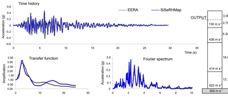
Figure 5. Comparison between EERA and SiSeRHMap (mod.3, stratigraphic response) on a 1-D model related to the third trainerVS–h

model regarding zone 2.

A number of iterations of 5–10 largely assures the con-vergence of a dynamic solution (the default value is: 10); in contrast the use of a number of iterations equal to zero entails a pure viscoelastic linear analysis. Nonetheless, a constant value of the damping ratio is assumed for rigid bedrock. This value is attributed both to the fixed rigid bedrock and to the rigid bedrock resulting from non-rigid bedrock (the default value is: 0.01). For the zones characterized by outcropping rigid rock, the seismic response is automatically referred to the input motion.

The aforementioned process can be iterated using more as-signed input motions; in this case the code is able to gen-erate the average seismic responses constituting the train-ing models used in the followtrain-ing meta-modelltrain-ing process. However, the smoothed responses, generated by the trained meta-model, suggest a better performance for input motions with the acceleration response spectra nearest, or matched, to the simplified code design spectra. On this subject, the multi-input motion mode performs the stratigraphic seismic response analysis for each input motion on all theVS–h se-lected profiles in a separate way. Therefore, average accel-eration response spectra are obtained from a set of output acceleration response spectra computed for each zone; these average spectra are the trainer models used in the subsequent meta-model procedure. However, it is worth noting, as previ-ously stated, that better performances of the meta-model are given using input motions that provide an average response spectra matched (or fitted) on the design code spectra shape (a complete example is illustrated in Fig. 8).

In the stratigraphic response module, an additional module “view signal” (Fig. 6) is associated in or-der to plot the time history signal (acceleration and strain) and spectra (transfer function, Fourier spectra, re-sponse spectra). (Some input and output files are reported in the Supplement folders: INPUT\Dynamic_properties; OUTPUT\mod3_Seismic_Response.)

3.2 “Emul-spectra”: adaptive simulation model

Emul-spectra,9, are a numerical adaptive model capable of emulating the theoretical stratigraphic seismic response. In this way, this model assumes a key role promoting the hybrid evolution of the procedures in SiSeRHMap.

The Emul-spectra model is introduced here and it stems from the previous experience of Grelle et al. (2014) in which hypotheses relating to the behaviour assumed by combina-tions of multi-parametric funccombina-tions were introduced with the aim of obtaining good performances in the fitting of the ac-celeration response spectra. In Emul-spectra, the natural in-fluence on the spectral-trends of some main physical parame-ters are largely taken into consideration, confirming previous studies regarding principal component analysis (PCA). The physical parameters used as independent variables in Emul-spectra are (i) the average shear wave velocity of the near-surface lithodynamic unit,VS(up); (ii) the elastic fundamental period of the sequence,Tf, and (iii) the period,T. Its analyt-ical form is

9= x1

VS(up)(1+x2T2)

+K x

Tflog(VS(up))

3

exp

(x4Tf+x5T )2 (Tf+x6T ) x7_log_(VTf

S(up))

log(1+T2) + x8 Tf

T V_S(up)2 , (14)

(10)

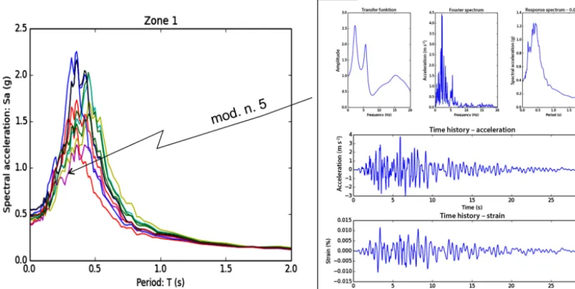
Figure 6. Example of the Stratigraphic seismic response set of zone 1 with 0.05 damping; for this set, the graphics plotted of the signal view

module related to the fifth trainerVS–hmodel are also shown. In the analysis (all zones), the equivalent stress ratio is obtained by Eq. (13),

taking into consideration a magnitude of 6.4.

value of 0.01 s and theVS(up)is set equal to the corresponding rigid bedrock.

The three component functions, summed to define Emul-spectra (Eq. 14), have specific and different roles in the fit-ness performance of the model. To this regard, and consid-ering 9 as being dependant onT, it is worth highlighting that (i) the first component has the role of “bed function” because it is the platform of the other component functions due to the fact that it greatly controls the intercept at the zero-period (Peak Ground Acceleration, PGA) and the tail fitting values; (ii) the second component is the “modal func-tion” that controls the fitting peak values in the modal shape; and (iii) the third component is the “PGA-correction func-tion”, which corrects the initial values permitting a more ac-curate fitting of the PGAs. In the bed function, the intercept (PGA) is inversely dependent on VS(up), although an addi-tion or subtracaddi-tion that is sign x8-coefficient dependent, is specifically performed by the PGA-correction function. The latter, in relation to the trend shown between Tf and PGA in the seismic response of a specific zone, permits taking into account the possible known non-linear effect to decre-ment the spectral values at high frequencies (low periods). The modal function is the core of the Emul-spectra adaptive model. It is a exponential equation capable of reproducing a symmetrical/asymmetrical modal or subordinated bimodal shapes generally shown by acceleration seismic responses in a large spectral range (e.g. in Fig. 7), as well as in the multi-input probabilistic way (Fig. 8). The modal function, which combines the parameters VS(up) andTf in a different way, permits a chasing of the various peak-trend distributions by zones as well as possible single spectral behaviours or

possi-ble non-peak-trend conditions due to the different influences of the non-linear responses. The modal scaling factor,K, acts only on the modal function. It is usually assumed to be equal to 1.00 and can be changed after calibration in order to scale the peaks.

(11)

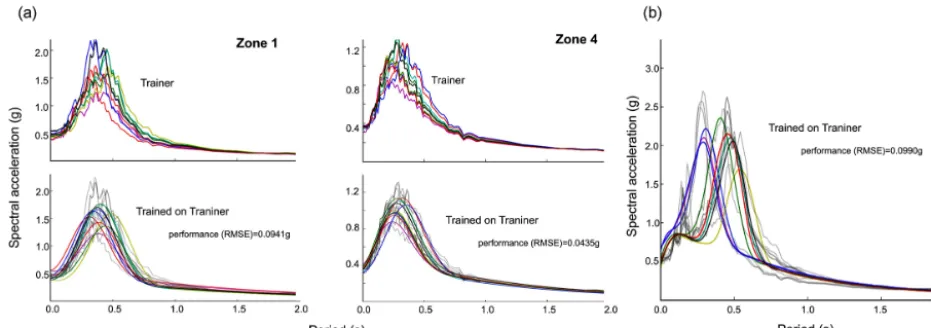
Figure 7. Performance of Emul-spectra: (a) stratigraphic seismic response with a damping of 0.05 regarding some trainerVS–hprofiles

of the SRS (all graphics are reported in the Supplement). The resulting performance defined by RMSE (g) are zone 1=0.0941; zone 2=0.0862; zone 3=0.0544; zone 4=0.0435; zone 5=0.0370; zone 6 (non rigid rock in outcropping)=0.0032; zone 7 (rigid rock in outcropping)=0.0045; zone 8=0.0394 (b) example on stratigraphic seismic responses that show a large spectral variability; the trainer spectra are obtained by the notable increasing of the top-layer thicknesses in the zone 1 models.

The EA is a meta-heuristic method based on an evolution-ary elitism of the offspring solutions that mutate up to satis-fying or converging into a predefined fitness condition. The fitness of the solutions is defined by the fitting error, which is expressed in terms of a mean square error (MSE). The EA is constituted by two breeding levels. In the first level, the off-spring solutions are generated according to a corresponding Gaussian distribution in which the mean values represent-ing the initial guesses population (low range parental) and corresponding standard deviations are supplied. In an itera-tive way, in the first level, only the population of offspring solutions, which shows a fitness better than the previously encountered solutions, is allowed to pass to the second level in accordance with the elitism process. The number of pro-creations is four (fixed) and for each successive generation the probable parental affinity is increased (Appendix B). The elitism process is reset (mass extinction) when an assigned number of population solutions is reached and the conver-gence has not been reached yet. The converconver-gence event oc-curs when an incremented assigned initial (minimum) error targetEtargis found. This error is increased by a assigned ra-tio (the default value is 0.01) at the end of the second breed-ing level when the process returns to the first breedbreed-ing level. The assigned value of the initial error target depends on the shape of the training seismic response curves in reference to the shape ability of the Emul-spectra model. However, the fitting, and consequently the Etarg value, can be dependent on the number of the randomly selected models, Nm, and on the number of the lithodynamic units present in the sequence, Nl. Taking this aspect into account, the default values ofEtarg are empirically defined, for each zone, as follows:

Etarg =

(Nm×Nl)

1000 . (15)

The choice of an appropriateEtargavoids a long computa-tional time or, in contrast, the occurrence of premature con-vergences.

Optionally, in the meta-model module (mod4), it is pos-sible to select the zone where an additional computation of “refinement” can be performed. This re-processing may be run when the fit or the shape regression curves are not con-sidered satisfactory by the operator. The new processing can be performed using the initial guess parameters obtained in the previous processing and new standard deviation values, as well as a new lowerEtarg, can be assigned.

4 GCM maps executor: mod.5

(12)

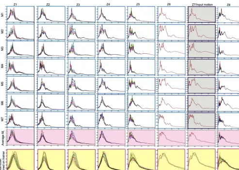
Figure 8. Example of meta-model processing for the SRS using seven input motions having average spectrum matched on an unamplified

design spectrum. This last corresponding to the average spectrum of the zone Z7 where the rigid rock outcrops.

4.1 Stratigraphic seismic response mapping

For every geographic x, y point, the GCM is able to asso-ciate a correspondingj-zone and consequently also the rel-ative parameters, processes, and information deriving from the previous modules. In this second phase, the GCM pro-ceeds to configure itself using the common physic bases and hypothesis assumed in the construction and parameterization of the trainerVS–hprofiles (Sect. 2.3). These are as follows: i. The average shear wave velocity,V¯Si(x,y), of the

litho-dynamic units, which is computed in accordance with Eq. (10); it assumes a value of zero where the lithody-namic is not present in the layer. In addition, if non-rigid bedrock is present at the bed of the sequence, the GCM generates then-cover layer in which the hn(x,y) andVSn(x,y)are defined in accordance with Eq. (9).

ii. The fundamental period Tf(x,y) is computed in

accor-dance with Eq. (11). In addition, where the rock is out-cropped, the fundamental period assumes a value of 0.01 s.

iii. In each zone, the GCM recognizes the average shear wave velocity of the nearest surface lithodynamic unit

VSup(x,y).

Once the GCM is parameterized, it is able to define the hy-brid stratigraphic seismic response (Fig. 8) by solving the numerical model Emul-spectra (Eq. 14) that in this context assumes the form:

6(T )(x,y)= f

(T ) , VSup(x,y), T0(x,y)

, (x1)j. . .(x8)j , (16) where the periodT assumes the values in the spectra inter-val for which Emul-spectra have been trained. The GCM maps executor computes the hybrid seismic response using the same period used in the meta-model training.

(13)

Figure 9. Set of seismic response maps for different periods. The combined effect of the stratigraphic and topographic features are shown at

the top of the figure; StR is the stratigraphic seismic response, TA is the topographic amplification and SR is the seismic response.

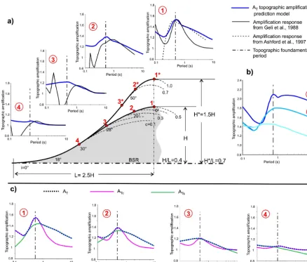
4.2 Topographic amplification mapping

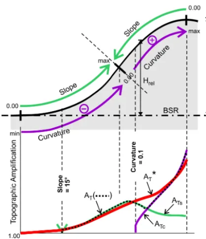
A prediction model has been developed based on pre-existing studies and simulations on the effects of topographic ampli-fication on seismic motion (Geli et al., 1988; Ashford et al., 1997; Maufroy et al., 2012, 2015). This model, trained on 2-D regular reliefs and balanced on 3-D landforms, aims at predicting the spatial amplification effect on the seismic re-sponse of reliefs, considering them to be constituted by ho-mogeneous material. To this scope, digital topographic at-tributes are used to introduce morphometric variables into the model. These are (i) digital elevation model, DEM (DTM_30.txt); (ii) slope angle,i(slope_30.txt), which is the arctangent of the first derivate of the DEM; and (iii) cur-vature,c (curvature_30.txt), which is the second derivative of the DEM. The latter is the inverse of the ray curvature, which is expressed in terms of a resolution unit ratio. There-fore, a positive value of the curvature represents convex fea-tures, such as ridges or edges, while a negative value indi-cates concave features, such as a valley. A geometric trend of the curvature and slope along a typical profile relief (the

upper part of Fig. 10) illustrates that the curvature assumes a greater value on the ridge, where the slope is minimum or near to zero, and the curvature assumes a zero value where the slope angle is greater. Towards the valley, the slope angle decreases while the curvature assumes negative values down to the minimum. The curvature is expressed in terms of the maximum values in relation to the 3-D minimum curvature radius, which implicates that the topographic amplification model tends to predict the maximum amplification associ-ated with the transversal polarized motion of the relief.

On the aforementioned bases, the prediction model of topographic amplification is a spatial–frequency dependent model constituted by a combination of the two sub-models (the lower part of Fig. 10). Taking into account a generic (x, y) point,ATcis the prediction model for the topographic amplification in ridge/edge regions:

ATc=1+c ηt e−2ηt+A1c ηt2e

−A2ηt2+ A3ηte √

(14)

Figure 10. The behaviour components of the topographic

amplifi-cation model in relation to the distribution of the GIS-topographic attributes (DEM, slope, and curvature) along an isolated half-relief.

andATsis the prediction model for the topographic amplifi-cation along the slope surface:

ATs=1+

rH

1+ B1c

2√πe

−B2η2t(1+c)+B3logηt

(1+sin2i) i

−rH o

, (18)

whererH =H /HRand it is the relief ratio in whichH and HR are, respectively, the local slope height and the relief height, both of which are taken into consideration by the basal surface of relief (BSR) whereH=0.A1,A2,A3and B1,B2,B3are the calibration parameters defined on the re-sults obtained by the numerical model analysis of the 2-D homogeneous relief (discussed below in this section); for Eq. (17), a subsequent light calibration on real 3-D cases (Sect. 4.2.1) is also affected. Hence, the dimensionless fre-quency, defined as slope height/wavelength, is

ηt = H VSRegT

, (19)

where theVSReg is the regional shear wave velocity. Finally,

the topographic amplificationAT is the maximum value of ATcandATsfor each (x, y) point.

SiSeRHMap permits the definition of the BSR in relation to features of the topographic area (Appendix C), while the regional shear wave velocity must be assigned. This repre-sents the average shear wave velocity of the rigid material constituting the relief(s), that can be different (frequently

greater) to the shear wave velocity of the rigid bedrock as-sumed in the stratigraphic response analysis. Thus, in SiS-eRHMap, the topographic sub-module permits the simula-tion of the 3-D surface amplificasimula-tion mainly on the basis of morphometric data and using an assigned uniform stiffness of the reliefs with the task of shifting the frequency distribu-tion of the amplificadistribu-tion data.

In general terms, the behaviour of theATcand theATs de-pends on the curvature and on the slope angle topography attributes, which, in turn, depend on the value of the spatial resolution unit as well as the elevation resolution (sampling altitude value). In order to take into account these conditions, the prediction models are calibrated on grid curvature data related to the spatial resolution unit of 30 m, which can be 1 order of magnitude higher than the resolution unit of the stratigraphic response (Eq. 4). In order to meet this assump-tion, a specific computational algorithm within the method excludes the natural ripples of the slope, which can be con-fused with ridges; in addition, the aforementioned assump-tion is sustained by the fact that the amplificaassump-tion of low rigid ridges (less than 30 m in height) occurs in frequencies that usually have very little effect on buildings. The algo-rithm necessitates a recognition of the complete topographic features of the region that is the subject of the stratigraphic response analysis; in some cases, this aspect involves taking into consideration an area much larger than one object of the stratigraphic response analysis. Subsequently, the algorithm performs an extracting, a georeferencing, and a resolution adaptation to the smaller target area that corresponds to the stratigraphic response area. In addition, the output grid-maps are Gaussian smoothed using a calibrated standard deviation value (expressed in the number of the resolution units) pending on the elevation resolution previous used for the de-velopment of the input topographic attribute maps. The cali-bration function derives from a sensibility analysis based on the invariant of the output data.

(15)

and it is predominant on the curvature zone (e.g. ridge or to-pographic border), while theATsmodel is predominant along the slope, as expected. This last model defines the amplifica-tion curve for high periods, in all the cases.

For some corresponding positions along the surface of the relief, the comparison with the numerical simulation per-formed by Geli et al. (1988) shows (Fig. 11) that the to-pographic prediction model, AT, is able to perform an ad-equate and efficient overlap, such as in comparison to the topographic edge feature (Ashford et al., 1997). An applica-tion in real areas (Fig. 12) illustrates the performance and the ability of the code to resolve the topographic model, by way of a preliminary definition of the BSR and the relief ratio,

rH. The mapping restitution process provides for a computa-tional optimization, mainly aimed at minimizing the unrea-sonable concentration of high values. These high values are caused by natural roughness, in addition to an anomaly in the base-digital map. The computational optimization, ofATin AT*, consists in the smoothed numerical bass cut of the slope angle<15◦, curvature>0.1, andHR<30 m.

The simplified frequency-dependent topographic amplifi-cation model, reported in Eqs. (17) and (18), is mainly fo-cused on the peak/ridge amplification effect (position 1 in Fig. 10) that is the greatest effect in the relief. The predic-tion accuracy on the slopes is the result of the progressive spatial smoothing of the topographic amplification and the conservative approach, too. The latter does not admit deam-plification. Diversely, it admits a suitable overmatch (overes-timation) in almost the entire spectral window. In this way, it gives the possibility to preserve an adequate prediction trend for irregular reliefs too. This aspect should be seen in light of the fact that the values of the slope topographic amplifi-cations are generally lower than those that occur in the peak zones.

4.2.1 Validation

Differently to the meta-model process at the base of the stratigraphic seismic response, the topographic model may not be trained on local specified cases of theoretical effects. The topographic model is based on surface 3-D-depending variables (DEM, slope, and curvature) that define the shape of relief(s) and, in general, of the terrain conformation. Therefore, this model was built and calibrated in order to take into account substantial case studies of hilly mountain sceneries which are prone or susceptible to seismic topo-graphic effects.

Bearing in mind that the strong natural spatial changing of topographic attributes influences the efficacy of the to-pographic amplification model of SiSeRHMap, some vali-dation tests were performed on real areas in order to verify the accuracy and robustness of its predictions. Two real hilly mountain areas were selected due to (1) their setting diversity and (2) the availability of in depth analysis, in terms of ex-perimental characterizations and numerical simulations,

car-ried out by other authors. The comparison cases (Fig. 13) regard: (i) the Albion Plateau area (France) (Maufroy et al., 2012, 2015) – a topographically articulate area constituted by hilly reliefs with complex shapes and with different direc-tions of their stretching axis; and (ii) the Narni relief (Italy) – a well-defined and partially isolated asymmetric relief, ap-proximately 1300 m long and with variable heights and basal widths.

In the first case (Fig. 13a), a 3-D numerical simulation of the topographic amplification was performed on the cen-tral part (target area) of the Albion Plateau area where 200 random double-couple point sources (fault plains modelling) were considered at approximately 4 km depth, in a homoge-neous subsoil half-space. In this way, waves with different in-cidences and intensities were contemplated. The simulation analysis was performed using a 3-D partly staggered finite difference code (Cruz-Atienza 2006). Moreover, the elas-tic and isotropic subsoil medium was modelled with shear and compression wave velocities of 3000 and 5000 m s−1, and a density of 2.6 g cm−3. Specifications on the process-ing modality and parameterization are reported in Maufroy et al. (2012). The comparison in the frequency domain was performed in terms of wave lengths in different representa-tive points regarding different topographic real features. The points and the chosen frequency are identical to those re-ported in Maufroy et al. (2015).

The results provided by the topographic model in SiS-eRHMap demonstrate how its predicted horizontal spectral amplifications are mainly included between the 50th and 84th percentile of the amplification values resulting from a nu-merical multi-source simulation for each of the five cases (Fig. 13a). In addition, it should be noted that the spectral peaks match the tendency of the numerical simulation. The matching is more evident in the ridge of the relief where the topographic amplification is greater; the deamplification ef-fects shown in the slope perched valley and bottom valley are predicted as a non-amplification effect in observance of the nature and the character of the proposed model.

(16)

re-1582 G. Grelle et al.: SiSeRHMap v1.0

Figure 11. Performance of the topographic prediction model,AT, along an isolate half-relief; this is similar to that used in the numerical

simulation by Geli et al. (1988). (a) The simulation considers vertical incident SH waves; in the same way, the Ashford et al. (1997) simulation analysis regards the ridge of the relief with a slope angle of 90◦; (b) topographic prediction projected on a more pronounced relief; (c) topographic prediction modelATillustrated in term of combined shape ofATc andATs models. The topographic fundamental

periods is corresponding toH /λ=0.2 (Geli et al., 1988.

gards two simplified geometrical models characterized by a uniform relief with VS=1400 m s−1, a double layer re-lief withVS=2000 m s−1for the outcropping top layer, and VS=1400 m s−1 for the bed layer; the same authors report that the relief rock material is constituted by massive lime-stone with diffused fracture patterns at the near surface. Con-sidering these models, two regional shear wave velocities,

VSReg, of 1500 and 2000 m s

−1_{, were used for the simulation} by the topographic model of SiSeRHMap. The results show a migration to high frequency that occurs when the regional shear velocity increases; this effect appears less evident for the peak that protrudes on the plain (3-D shape). The topo-graphic computing module of SiSeRHMap was applied on an area that includes approximately 1500 m of the relief’s length. However, the comparison was focalized on the first part, at approximately 700 m of the protruding area, where

experimental and numerical simulation data were available in order to perform the validation analysis. The extraction of the 2-D spectral amplification factor along the edge and ridge of the relief highlights the 3-D nature in the prediction anal-ysis of the model. On this subject, the local saddle feature (inB andB*) along the ridge conserves high amplification values on the edge and a substantial decreasing at the central ridge (crest), reported in Fig. 13b.

The comparison analysis takes into consideration the to-pographic amplification distribution along the ridge profile, obtained assuming a VSReg of 2000 m s

(17)

direc-Figure 12. Example of topographic amplification computed on a real hill-mountain area of southern Italy: blue box is the automatic splitting

map of the urbanized area of the village of Montefusco.

tional (transversal to relief) horizontal amplification of the average SSRs values in the zone subject to seismic stations at the top of the relief. The 2-D numerical simulation, with an amplification from 5 to 8 Hz, does not match the SSR values. With regards to the amplification results, they show spectral average values slightly greater by a factor of up to 3 and 4 for non-directional SSRs, respectively, and up to 2 for the to-pographic prediction model in SiSeRHMap; this last factor is also shown in the 2-D numerical analysis. On this specific topic and in agreement with scientists working on this area (Lovati et al., 2011; Massa et al., 2012; Barani et al., 2014), it is possible to hypothesize a net overlapping spectra between the stratigraphic and the topographic effects. In support of the aforementioned effects, the spectral amplification results obtained by the HVSR analysis and the non-directional SSRs intervene showing peaks of fundamental periods (3 to 5 Hz) close to the directional SSRs values. A more detailed debate on this topic is reported in the discussion paragraph. 4.3 Design spectra mapping

The design spectra are obtained by the envelopment of the HSR in observance of the synthetic spectra drawn by the discontinuous function, which defines the elastic response in Euro Code 8 as well as in FEMA 356 (2000). The enve-lope technique used here needs to take into account the dis-crete nature of the hybrid seismic response. The technique (Fig. 14) consists in the following computational steps:

i. recognition of the period, Tp, showing the maximum value (peak) of the hybrid seismic response HSRmax; ii. computation of the mean,M, of the HSR values, which

are greater than the intercept HSR0value at periodT = 0.001 (≈PGA);

iii. computation of the meanMR andML of HSR values greater than M, respectively, to the right and left of HSRmax;

iv. in this way the characterized parameters of the design spectra are

a0=HSR0, (20)

f0=

HSRmax HSR0

, (21)

TB=Tp

1−

_M

ML NL

N

, (22)

TC=Tp

1+

_M

MR NR

N

, (23)

TD=1.6+(4HSR0) , (24)

(18)

Figure 13. (a) Albino Plateau area (France): SiSeRHMap multi-spectral topographic amplification maps shown in terms of wavelength,

λ, assuming aVSof 3000 m s−1and using a resolution in elevation of 20 m. Comparison in characterizing topographic points between the

map-extrapolated values and the results of 3-D simulation model (SHAKE 3D; Cruz-Atienza 2006); results of GIS-topographic amplification proxy, which is built and calibrated in this specific area (Maufroy et al., 2015). (b) Narni prominent hill (Italy): SiSeRHMap multi-spectral topographic amplification maps defined assumingVSof 1500 and 2000 m s−1; performance of the model along the edge and crest profile.

(19)

Figure 14. Enveloping model that creates the design spectrum; around it, the mapping distribution of the characteristic parameters of the

design spectra, are shown.

5 Discussion

The SiSeRHMap methodology platform is composed of in-terdependent computational modules and sub-modules that in turn assume a crucial role in the prediction and therefore in the expected performance. Specifically, its seismic response map-sets are the result of a series of conventional/non-conventional procedures (hybrid) that use combined models that are simplified in different degrees in order to simulate the seismic response of more or less complex environments. On this subject and keeping in mind the theoretical bases as well as the validation cases, it seems appropriate to give here a complete overview of the strengths as well as the approxi-mations and limitations of SiSeRHMap.

In general terms, the site seismic response of SiSeRHMap is defined as a 1-D stratigraphic effect, defined by trained meta-model, loaded with 3-D topographic effects in terms of the aggravation factor. An example is shown in Fig. 15; it re-gards the integration analysis of the Narni relief case consid-ering the 1-D seismic response of a depth-decreased fractur-ing model computed with SiSeRHMap in a probolistic way assuming a single zone with a normal distribution (twenty combinations) of the shear wave velocity and thickness of layers. This data distribution is supported by the average uni-form shear wave velocity proposed by Lovati et al. (2011) and Barani et. (2014) as well as by the local geological fea-tures (Storti and Salvini, 2001). The results shows a sub-stantial matching with the experimental spectral ratio data

referred to a strong motion data set (Sect. 4.1.1). However, in agreement with other authors (Sect. 1.2), the model may be limited when the mutual interaction of the two aforemen-tioned effects appears considerable. For example, the pos-sible influence of the topographic effect on the pospos-sible in-creasing of the non-linearity behaviour of the soils covering the reliefs is not contemplated, as well as the possible non-linear response of the reliefs when these are constituted by soft materials.

Nevertheless, considering the aforementioned topics in reference to the single aspects of the SiSeRHMap model, it is possible to affirm that

– The GCM, which is the geometrical computation frame for the model, does not preset the geometrical limita-tion. It exploits the advantage of the multi-layer GIS-building techniques. In the GCM, the lithodynamic unit is defined by non-linear/linear monotonic VS depth-depending laws calibrated via a regression analysis of the selected and spatial diffused data. Taking into con-sideration this feature, the high standard deviations pro-duced by localized clustered data may be diminished, inserting a new lithodynamic unit for this data.

(20)

seis-1586 G. Grelle et al.: SiSeRHMap v1.0

Figure 15. Seismic response by SiSeRHMap (linear analysis mode) in comparison to the SSR experimental analysis.

mic response is defined by a viscoelastic linear equiv-alent model with the same performance of similar mod-els/codes (Fig. 5); the conservative aptitude degree of these models is the object of different case studies and suggestions (e.g. in Adampira et al., 2015; Zidan, 2015). (ii) The seismic responses obtained by the meta-model process are affected by checked trainer errors (intrin-sic errors); in contrast the maps developed by the meta-model solving are affected by non-checked errors (pre-diction errors), that nevertheless have values compara-ble with the aforementioned checked errors. (iii) The maps generated by SiSeRHMap may suffer of substan-tial uncertainties when high complex subsoil features are present. The latter are summarized in the high slope degree of the interfaces (L/H <8–10 in Hasal and Iy-isan, 2014) and in general by sharp variation of the buried morphology. On these effects, it is noted that 1-D seismic response seems to be underperformed mainly at the edge of the valley (Gelagoti et al., 2010). Future developments of SiSeRHMap will focused on this sub-ject. (iv) Independence of site response to azimuth and the wave-incidence angles with subsoil interfaces. – The frequency dependant topographic prediction model

is based on the topographic response of simplified ho-mogeneous regular reliefs. However, its reliability in the prediction for real cases has been ascertained (Fig. 13). Specifically, the prediction performances match the third party results deriving from different topographic frameworks and input motion sources, which are ob-tained both via numerical simulations and experimental

analysis. The comparison, with the 3-D numerical sim-ulation in homogeneous material, highlights (Fig. 13a) that SiSeRHMap’s topographic spectral responses fall near the third quartile of normal output distributions for all different characterizing locations. The compar-ison with the results of the 3-D experimental analysis (Fig. 13b) confirm a relevant aptitude in the frequency range prediction of the topographic model. In addition, these cases highlight how epistemic uncertainty can be reduced assuming a calibratedVSReg, which is obtained

taking into consideration the experimental spectral ra-tio in the trial comparison analysis. For example, in the presence of a not well-known rigidity of the relief or in the presence of non-homogeneous material constitut-ing the relief, a local frequency calibration, usconstitut-ing also seismic signal noise or weak earthquake measurements (in single or multi-station recording mode), can be per-formed assuming a calibrate regional shear wave veloc-ity that may be different from that used for depth rigid material (e.g. equivalent to VSReg). To this regard, we

can report that the computational times for the cases of Fig. 13a and b are approximately 24 s (cell-size=2 m) and 3 s (cell-size=5 m), respectively.

(21)

sur-Figure 16. Comparison in some characterized points between the seismic response by SiSeRHMap and the Quake/W finite element method

on a cross section showed in Fig. 1.

veys in order to define the lithodynamic model. In this con-text, SiSeRHMap is more efficacious in some large specific subjects that, in general, characterize the seismic response. This can be summarized in: (i) the use of the local ade-quate shear wave velocity of the lithodynamic units deriving from the statistical regression analysis; (ii) the development of georeferenced multi-spectral seismic response maps via the solving of meta-modelled smoothed responses that

(22)

1588 G. Grelle et al.: SiSeRHMap v1.0 practices guided by experimental analysis. For

demonstra-tion purposes, a final comparison between SiSeRHMap and a physically based numerical analysis code was performed on the synthetic recurrent scenario. The Quake/W (GeoStu-dio 2007) is a 2-D geotechnical finite element (FEM) soft-ware, which takes into consideration dynamic shear-strain-dependent viscoelastic material using dynamic linear equiv-alent analysis. This software offers the possibility to be pa-rameterized using some of SiSeRHMap’s input: the shear modules increase with effective vertical stress and conse-quently with depth; in addition it gives the possibility to as-sume the equivalent shear strain ratio in relation to magni-tude. The comparison (Fig. 16) regards six points distributed along cross section A (trace in Fig. 1) in order to investi-gate different lithologies and topographic features. The input earthquake used in the comparison analysis is the same used in the stratigraphic response module (mod.3). This input mo-tion is properly scaled in order to produce in the check point a spectrum coherent with the deconvoluted 1-D spectrum at the same depth. The check point is placed under the covered layer in the flat zone, while the mesh is assumed with differ-ent dimensions in relation to the thickness of the layers.

The comparison analysis highlights how the hybrid re-sponse is close in amplification as well as coherent in fre-quency to the response provided by exclusively physically based models solved by the 2-D FEM code. In this way, the aptitude of the hybrid model of SiSeRHMap seems to have a good compromise both for the definition of theoretical an-alytical response and for satisfying the exigency to provide the synthetic spectra shape required by building design.

6 Conclusions

SiSeRHMap introduces a new method, defined as “hybrid”, which is capable of creating maps of seismic response based on concepts of simulation cases, training, and prediction.

The simulation (from mod.1 to mod.3) involves physic-numerical analysis consisting in a 1-D seismic response (mod.3), based on a linear-equivalent shear stress–strain model; this model performs onVS–hprofiles uniformly sam-pled in the GCM. The latter, in the first phase, is a structured-synthetic representation of the subsoil by layered lithody-namic units (mod.1 and mod.2). The training is the core of the method due to the fact that it provides its hybrid evo-lution in the stratigraphic seismic response. In this way, the adaptive prediction model, Emul-spectra, seems to show ro-bustness and efficacy features, while its accuracy is assured by the dedicated evolutionary algorithm (mod.4). The sec-ond phase of the GCM (mod.5) provides the mapped solu-tion of the Emul-spectra model and the validated 3-D topo-graphic prediction model, in order to produce map sets of hybrid seismic responses and their envelopment process with the design spectra. Therefore, the general model at the base of SiSeRHMap confers to it the attribute of a first compu-tational program that associates consolidated techniques of stratigraphic seismic response with advanced techniques re-garding numerical emulation models and their training. In this way, SiSeRHMap permits the obtainment of map data, which can be easily diffused and consulted.

Code availability

(23)

Appendix A: Stratigraphic Seismic Response module Module three computes the dynamic seismic response for a site model with infinitely extended horizontal covered lay-ers assuming a vertical propagation of polarized shear waves stemming from a viscoelastic rigid bedrock (Fig. A1). The non-linear-viscoelastic strain that depends on the dynamic behaviour of soils constituting the covered layers is com-puted using the equivalent linear-viscoelastic analysis. Here, the base assumption is the 1-D linear-viscoelastic propaga-tion of the shear wave in a homogeneous soil that is assumed as a Kelvin–Voigt solid in which the dynamic response is modelled using purely an elastic spring and a purely viscous dashpot (Kramer, 1996). For this model, the solution to the harmonic wave with a frequency ω, that provides the dis-placement u, as a function of depthz, and timet (Kramer, 1996), is

u(z, t )=Xexp[j (ωt+k∗z)] +Y exp[j (ωt−k∗z)], (A1) where the first and second terms represent the incident and reflected wave travelling; therefore X and Y are, respec-tively, the amplitudes of the incident wave in the negative

z-direction (upward) and reflected wave in the positive z -direction (downward). In addition, in Eq. (A1),k∗is the com-plex wave number related to the comcom-plex shear modulus,G∗, damping ratio,D, and mass unit weight,ρ, of the soil, with

k∗= ω V_S∗=

ω q

G∗

ρ

, (A2)

taking into consideration that the critical damping ratio, D, is related to the viscosity,η, by

ωη=2GD. (A3)

Here, it is reasonable to assume that the dynamic param-eters G andD are almost constant in the frequency range where the analysis is usually performed. Hence, it is possible to express the complex shear modulus in terms of the critical damping ratio instead of the viscosity:

G∗=G+j ωη=G(1−2D2+j2Dp1−D2₎ ∼

=G(1+2j D), (A4)

whereGcan be taken as being independent from frequency. Hence, from Eq. (A1), for the top and bottom interfaces of thei-layer with a thicknesshi(Fig. A1), it is possible to express the strain [(ui(0, t ), ui(hi, t )] in relation to the shear stress [(τi(0, t ), τi(hi, t )]in this way:

τi(z, t )=(Gi+j ωηi) δui

δz = j kiGi

Xexp[j (ωt+k_i∗z)]

+Y exp[j (ωt−k∗_iz)] exp(j ωt ). (A5)

Therefore, imposing the continuity condition in the inter-face, in generic time,t, the following occurs:

ui(hi)=ui+1(0)andτi(hi)=τi+1(0) (A6) obtaining the relations:

Xiexp(j ki∗hi)+Yi exp[−(j ki∗hi)] =Xi+1+Yi+1 (A7) k∗_i G∗_i Xiexp(j ki∗hi)+Yi exp[−(j ki∗hi)]

=k∗_i+1G ∗

i+1(Xi+1+Yi+1) . (A8) For this later relation it is possible to express:

αi=

k∗_i G∗_i k_i∗₊₁G∗_i₊₁≡

s ρiG∗_i ρi+1G∗_i+1

(A9)

and therefore to define the following recurrence formulation:

Xi+1= 1 2

Xi(1+αi)exp(j ki∗hi)

+Yi(1−αi)exp−(j ki∗hi), (A10) Yi+1=

1 2

Xi(1−αi)exp(j ki∗hi)

+Yi(1+αi)exp−(j ki∗hi). (A11) At the top of the first layer in the free surface condition, the shear strength isτ1(0)=0. Hence, Eq. (A5) defines that the amplitude of incidentX1and reflectY1waves are equal. Therefore, once the shear module and damping in each layer is known, it is possible to compute the value of genericXi and Yi within the sequence for an assigned range of fre-quency. The computation is performed assuming the itera-tive recursive calculation starting from the free surface where

X1=Y1=1 until the input (base) layer is reached. In this way, the transfer function for the incident and refract compo-nent of motion on the surface of theilayer can be obtained from equations

Xi=xi(ω)X1, (A12)

Yi=yi(ω)Y1≡yi(ω)X1. (A13)

Using Eq. (A1), the above transfer functions permit ex-pressing the ratio of the amplitude of the harmonic motion in terms of displacement, velocity, and/or acceleration be-tween two layers for each frequency assumed. Therefore, the resultant transfer function, TF(ω)that defines the amplifica-tion between the rock surface associated with layer (n) and the upper-surface of a cover layer (i) or within the generic cover layer (i), when a sub-layer division of the column is performed, is defined as

TF(n,i)(ω)=

xi(ω)+yi(ω) xn(ω)+yn(ω)

.. (A14)