R E S E A R C H
Open Access
Computing eigenvalues and Hermite
interpolation for Dirac systems with
eigenparameter in boundary conditions
Mohammed M Tharwat
**Correspondence: [email protected] Department of Mathematics, Faculty of Science, King Abdulaziz University, Jeddah, Saudi Arabia Department of Mathematics, Faculty of Science, Beni-Suef University, Beni-Suef, Egypt
Abstract
Eigenvalue problems with eigenparameter appearing in the boundary conditions usually have complicated characteristic determinant where zeros cannot be explicitly computed. In this paper we use the derivative sampling theorem ‘Hermite
interpolations’ to compute approximate values of the eigenvalues of Dirac systems with eigenvalue parameter in one or two boundary conditions. We use recently derived estimates for the truncation and amplitude errors to compute error bounds. Using computable error bounds, we obtain eigenvalue enclosures. Examples with tables and illustrative figures are given. Also numerical examples, which are given at the end of the paper, give comparisons with the classical sinc-method in Annaby and Tharwat (BIT Numer. Math. 47:699-713, 2007) and explain that the Hermite
interpolations method gives remarkably better results. MSC: 34L16; 94A20; 65L15
Keywords: Dirac systems; eigenvalue problems with eigenparameter in the boundary conditions; Hermite interpolations; truncation error; amplitude error; sinc methods
1 Introduction
Letσ> andPWσbe the Paley-Wiener space of allL(R)-entire functions of exponential
typeσ. Assume thatf(t)∈PW
σ⊂PWσ. Thenf(t) can be reconstructed via the
Hermite-type sampling series
f(t) =
∞
n=–∞
f
nπ σ
Sn(t) +f
nπ σ
sin(σt–nπ)
σ Sn(t)
, (.)
whereSn(t) is the sequences of sinc functions
Sn(t) :=
⎧ ⎨ ⎩
sin(σt–nπ) (σt–nπ) , t=
nπ σ ,
, t=nσπ.
(.)
Series (.) converges absolutely and uniformly onR,cf.[–]. Sometimes, series (.) is called the derivative sampling theorem. Our task is to use formula (.) to compute eigen-values of Dirac systems numerically. This approach is a fully new technique that uses the recently obtained estimates for the truncation and amplitude errors associated with (.),
cf.[]. Both types of errors normally appear in numerical techniques that use interpo-lation procedures. In the following we summarize these estimates. The truncation error associated with (.) is defined to be
RN(f)(t) :=f(t) –fN(t), N∈Z+,t∈R, (.)
wherefN(t) is the truncated series
fN(t) =
|n|≤N
f nπ σ
Sn(t) +f
nπ σ
sin(σt–nπ)
σ Sn(t)
. (.)
It is proved in [] that iff(t)∈PWσ andf(t) is sufficiently smooth in the sense that there
existsk∈Z+such thattkf(t)∈L(R), then, fort∈R,|t|<Nπ/σ, we have
RN(f)(t)≤TN,k,σ(t)
:= ξk,σEk|sinσt| √
(N+ )k
(Nπ–σt)/ +
(Nπ+σt)/
+ξk,σ(σEk+kEk–)|sinσt|
σ(N+ )k
√
Nπ–σt+ √
Nπ+σt
, (.)
where the constantsEkandξk,σ are given by
Ek:=
∞
–∞
tkf(t)dt, ξ k,σ:=
σk+/
πk+√ – –k. (.)
The amplitude error occurs when approximate samples are used instead of the exact ones, which we cannot compute. It is defined to be
A(ε,f)(t) =
∞
n=–∞ f nπ σ –f
nπ
σ
Sn(t)
+ f nπ σ –f
nπ
σ
sin(σt–nπ)
σ Sn(t)
, t∈R, (.)
wheref(nσπ) andf(nσπ) are approximate samples off(nσπ) andf(nσπ), respectively. Let us assume that the differencesεn:=f(nσπ) –f(
nπ
σ ),εn :=f(n
π σ ) –f(
nπ
σ ),n∈Z, are bounded by
a positive numberε,i.e.,|εn|,|εn| ≤ε. Iff(t)∈PWσ satisfies the natural decay conditions
|εn| ≤
f nπ σ
, εn≤f
nπ σ
, (.)
f(t)≤ Mf
|t|α+, t∈R–{}, (.)
<ω≤, then for <ε≤min{π/σ,σ/π, /√e}, we have, [],
A(ε,f)∞≤ e /
σ(ω+ )
√
e( +σ) +(π/σ)A+Mf
ρ(ε)
+σ+ +log()Mf
where
A:=σ
π
f()+Mf
σ π
ω
, ρ(ε) :=γ + log(/ε), (.)
andγ:=limn→∞[kn=k–logn]∼= . is the Euler-Mascheroni constant.
The classical [] sampling theorem of Whittaker, Kotel’nikov and Shannon (WKS) for f ∈PW
σ is the series representation
f(t) =
∞
n=–∞ f
nπ
σ
Sn(t), t∈R, (.)
where the convergence is absolute and uniform onRand it is uniform on compact sets
ofC,cf.[–]. Series (.), which is of Lagrange interpolation type, has been used to com-pute eigenvalues of second-order eigenvalue problems; see,e.g., [–]. The use of (.) in numerical analysis is known as the sinc-method established by Stenger,cf.[–]. In [, ], the authors applied (.) and the regularized sinc-method to compute eigenvalues of Dirac systems with a derivation of the error estimates as given by [, ]. In [] the Dirac system has an eigenparameter appearing in the boundary conditions. The aim of this pa-per is to investigate the possibilities of using Hermite interpolations rather than Lagrange interpolations, to compute the eigenvalues numerically. Notice that, due to Paley-Wiener’s theorem [],f ∈PWσ if and only if there isg(·)∈L(–σ,σ) such that
f(t) =√ π
σ
–σ
g(x)eixtdx. (.)
Thereforef(t)∈PWσ,i.e.,f(t) also has an expansion of the form (.). However,f(t)
can be also obtained by the term-by-term differentiation formula of (.)
f(t) =
∞
n=–∞ f
nπ
σ
Sn(t), (.)
see [, p.] for convergence. Thus the use of Hermite interpolations will not cost any additional computational efforts since the samplesf(nσπ) will be used to compute both f(t) andf(t) according to (.) and (.), respectively.
Consider the Dirac system which consists of the system of differential equations
u(x) –r(x)u(x) =λu(x), u(x) +r(x)u(x) = –λu(x), x∈[, ] (.) and the boundary conditions
αu() –αu() = –λαu() –αu(), (.)
βu() –βu() = –λβu() –βu(), (.)
wherer(·),r(·)∈L(, ) andαi,βi,αi,βi∈R,i= , , satisfying
α,α= (, ) orαα–αα>
and
β,β= (, ) orββ–ββ>
.
The eigenvalue problem (.)-(.) will be denoted by (r,α,β,α,β) when (α,α)= (, )= (β,β). It is a Dirac system when the eigenparameterλappears linearly in both boundary conditions. The classical problem whenα=α=β=β= , which we denote by(r,α,β, , ), is studied in the monographs of Levitan and Sargsjan [, ]. Annaby and Tharwat [] used Hermite-type sampling series (.) to compute the eigenvalues of problem(r,α,β, , ) numerically. In [], Kerimov proved that(r,α,β,α,β) has a
de-numerable set of real and simple eigenvalues with±∞as the limit points. Similar results
are established in [] for the problem when the eigenparameter appears in one condition, i.e., whenα=α= , (β,β)= (, ) or equivalently when ( α,α)= (, ) andβ=β= , where also sampling theorems have been established. These problems will be denoted by
(r,α,β, ,β) and(r,α,β,α, ), respectively. The aim of the present work is to compute the eigenvalues of(r,α,β,α,β) and(r,α,β, ,β) numerically by the Hermite inter-polations with an error analysis. This method is based on sampling theorem, Hermite interpolations, but applied to regularized functions hence avoiding any (multiple) inte-gration and keeping the number of terms in the Cardinal series manageable. It has been demonstrated that the method is capable of delivering higher-order estimates of the eigen-values at a very low cost; see []. In Sections and , we derive the Hermite interpolation technique to compute the eigenvalues of Dirac systems with error estimates. We briefly derive some necessary asymptotics for Dirac systems’ spectral quantities. The last section contains three worked examples with comparisons accompanied by figures and numerics with the Lagrange interpolation method.
2 Treatment of
(r,
α
,β
,α
,β
)In this section we derive approximate values of the eigenvalues of (r,α,β,α,β). Re-call that(r,α,β,α,β) has a denumerable set of real and simple eigenvalues,cf.[]. Let
ϕ(·,λ) = (ϕ(·,λ),ϕ(·,λ))be a solution of (.) satisfying the following initial:
ϕ(,λ) =α+λα, ϕ(,λ) =α+λα. (.)
HereAdenotes the transpose of a matrixA. Sinceϕ(·,λ) satisfies (.), then the eigen-values of the problem(r,α,β,α,β) are the zeros of the function
(λ) :=β+λβ
ϕ(,λ) –
β+λβ
ϕ(,λ). (.)
Similarly to [, p.],ϕ(·,λ) andϕ(·,λ) satisfy the system of integral equations
ϕ(x,λ) = –
α+λα
sinλx+α+λα
cosλx+Tϕ(x,λ) +Tϕ(x,λ), (.)
ϕ(x,λ) =
α+λα
sinλx+α+λα
cosλx–Tϕ(x,λ) +Tϕ(x,λ), (.)
whereTiandTi,i= , , are the Volterra operators defined by
Tiu(x,λ) :=
x
sinλ(x–t)ri(t)u(t,λ)dt,
Tiu(x,λ) :=
x
cosλ(x–t)ri(t)u(t,λ)dt, i= , .
For convenience, we define the constants
c:=max
|α|+|α|,α+α, c:=
r(t)+r(t)dt,
c:=cc, c:=cexp(c),
c:=max|β|+|β|,β+β, c:=cc.
(.)
Defineh(·,λ) andh(·,λ) to be
h(x,λ) :=Tϕ(x,λ) +Tϕ(x,λ), h(x,λ) := –Tϕ(x,λ) +Tϕ(x,λ). (.)
As in [] we split(λ) into two parts via
(λ) :=G(λ) +S(λ), (.)
whereG(λ) is the known part
G(λ) :=β+λβ
–α+λα
sinλ+α+λα
cosλ
–β+λβ
α+λα
sinλ+α+λα
cosλ (.)
andS(λ) is the unknown one
S(λ) :=β+λβ
h(,λ) –
β+λβ
h(,λ). (.)
Then the functionS(λ) is entire inλfor eachx∈[, ] for which,cf.[],
S(λ)≤c +|λ|e|λ|, λ∈C. (.)
The analyticity ofS(λ) as well as estimate (.) are not adequate to prove thatS(λ) lies in a Paley-Wiener space. To solve this problem, we will multiplyS(λ) by a regularization factor. Letθ> andm∈Z+,m≥, be fixed. LetF
θ,m(λ) be the function
Fθ,m(λ) :=
sinθ λ θ λ
m
S(λ), λ∈C. (.)
We chooseθsufficiently small for which|θ λ|<π. More specifications onm,θwill be given latter on. ThenFθ,m(λ), see [], is an entire function ofλwhich satisfies the estimate
Fθ,m(λ)≤ cm
c( +|λ|) ( +θ|λ|)m e
|λ|(+mθ), λ∈C. (.)
Moreover,λm–F
θ,m(λ)∈L(R) and
Em–(Fθ,m) =
∞
–∞ λm–F
θ,m(λ)
where
ξ:=
θm–
+ m– θ+ θ+ mθ– m m– m+ m– +
θ(θ+ m– )
(m– m+ m– )(m– )(m– )
.
What we have just proved is thatFθ,m(λ) belongs to the Paley-Wiener spacePWσ with σ= +mθ. SinceFθ,m(λ)∈PWσ ⊂PWσ, then we can reconstruct the functionsFθ,m(λ)
via the following sampling formula:
Fθ,m(λ) =
∞
n=–∞
Fθ,m
nπ
σ
Sn(λ) +Fθ,m
nπ σ
sin(σ λ–nπ)
σ Sn(λ)
. (.)
LetN∈Z+,N>m, and approximateFθ,m(λ) by its truncated seriesFθ,m,N(λ), where
Fθ,m,N(λ) := N
n=–N
Fθ,m
nπ
σ
Sn(λ) +Fθ,m
nπ σ
sin(σ λ–nπ)
σ Sn(λ)
. (.)
Since all eigenvalues are real, then from now on we restrict ourselves to λ∈R. Since
λm–F
θ,m(λ)∈L(R), the truncation error,cf.(.), is given for|λ|<Nσπ by
Fθ,m(λ) –Fθ,m,N(λ)≤TN,m–,σ(λ), (.)
where
TN,m–,σ(λ)
:=ξm–,σEm–|sinσ λ| √
(N+ )m–
(Nπ–σ λ)/+
(Nπ+σ λ)/
+ξm–,σ(σEm–+ (m– )Em–)|sinσ λ|
σ(N+ )m–
√
Nπ–σ λ+
√
Nπ+σ λ
. (.)
The samples{Fθ,m(nσπ)}
N
n=–N and{Fθ,m(n
π σ )}
N
n=–N, in general, are not known explicitly. So,
we approximate them by solving numerically N+ initial value problems at the nodes
{nπ σ }
N
n=–N. Let{Fθ,m(nσπ)}
N
n=–Nand{Fθ,m(n
π σ )}
N
n=–N be the approximations of the samples of {Fθ,m(nσπ)}Nn=–Nand{Fθ,m(nσπ)}
N
n=–N, respectively. Now we defineFθ,m,N(λ), which
approx-imatesFθ,m,N(λ)
Fθ,m,N(λ)
:=
N
n=–N
Fθ,m
nπ
σ
Sn(λ) +Fθ,m
nπ σ
sin(σ λ–nπ)
σ Sn(λ)
, N>m. (.)
Using standard methods for solving initial problems, we may assume that for|n|<N,
Fθ,m
nπ
σ
–Fθ,m
nπ
σ
<ε, Fθ,m
nπ σ
–Fθ,m
nπ
σ
for a sufficiently smallε. From (.) we can see thatFθ,m(λ) satisfies the condition (.)
whenm≥ and therefore whenever <ε≤min{π/σ,σ/π, /√e}, we have
Fθ,m,N(λ) –Fθ,m,N(λ)≤A(ε), λ∈R, (.)
where there is a positive constantMFθ,mfor which,cf.(.),
A(ε) := e /
σ
√
e( +σ) +
π
σA+MFθ,m
ρ(ε)
+σ+ +log()MFθ,m
εlog(/ε). (.)
Here
A:=σ
π
Fθ,m()+
σ πMFθ,m
, ρ(ε) :=γ+ log(/ε).
In the following, we use the technique of [], where only the truncation error analysis is considered, to determine enclosure intervals for the eigenvalues; see also [, ]. Letλ∗
be an eigenvalue with|θ λ∗|<π, that is,
λ∗=Gλ∗+
sinθ λ∗ θ λ∗
–m
Fθ,m
λ∗= .
Then it follows that
Gλ∗+
sinθ λ∗ θ λ∗
–m
Fθ,m,N
λ∗
=
sinθ λ∗ θ λ∗
–m
Fθ,m,N
λ∗–
sinθ λ∗ θ λ∗
–m
Fθ,m
λ∗
=
sinθ λ∗ θ λ∗
–m
Fθ,m,N
λ∗–
sinθ λ∗ θ λ∗
–m
Fθ,m,N
λ∗
+
sinθ λ∗ θ λ∗
–m
Fθ,m,N
λ∗–
sinθ λ∗ θ λ∗
–m
Fθ,m
λ∗
and so Gλ∗+
sinθ λ∗ θ λ∗
–m
Fθ,m,N
λ∗≤sinθ λ
∗
θ λ∗
–mTN,m–,σ
λ∗+A(ε).
SinceG(λ∗) + (sinθ λ∗ θ λ∗ )
–mF
θ,m,N(λ∗) is given and |sinθ λ ∗
θ λ∗ |
–m(T
N,m–,σ(λ∗) +A(ε)) has
com-putable upper bound, we can define an enclosure forλ∗by solving the following system
of inequalities:
–sinθ λ
∗
θ λ∗
–mTN,m–,σ
λ∗+A(ε)≤Gλ∗+
sinθ λ∗ θ λ∗
–m
Fθ,m,N
λ∗
≤sinθ λ∗
θ λ∗
–mTN,m–,σ
Its solution is an interval containingλ∗, and over which the graph
Gλ∗+
sinθ λ∗ θ λ∗
–m
Fθ,m,N
λ∗
is squeezed between the graphs
–sinθ λ
∗
θ λ∗
–mTN,m–,σ
λ∗+A(ε) (.)
and sinθ λθ λ∗∗
–mTN,m–,σ
λ∗+A(ε). (.)
Using the fact that
Fθ,m,N(λ)→Fθ,m(λ)
uniformly over any compact set, and sinceλ∗is a simple root, we obtain, for largeNand sufficiently smallε,
∂ ∂λ
G(λ) +
sinθ λ θ λ
–m
Fθ,m,N(λ)
=
in a neighborhood ofλ∗. Hence the graph ofG(λ) + (sinθ λθ λ )–mFθ,m,N(λ) intersects the graphs
–|sinθ λθ λ|–m(TN,m–,σ(λ) +A(ε)) and|sinθ λθ λ |–m(TN,m–,σ(λ) +A(ε)) at two points with
abscis-saea–(λ∗,N,ε)≤a+(λ∗,N,ε) and the solution of the system of inequalities (.) is the interval
Iε,N :=
a–λ∗,N,ε,a+λ∗,N,ε
and in particularλ∗∈Iε,N. Summarizing the above discussion, we arrive at the following
lemma which is similar to that of [] for Sturm-Liouville problems.
Lemma . For any eigenvalueλ∗,we can find N∈Z+and sufficiently smallεsuch that
λ∗∈Iε,N for N>N.Moreover,
a–λ∗,N,ε,a+λ∗,N,ε→λ∗ as N→ ∞andε→. (.)
Proof Since all eigenvalues of(r,α,β,α,β) are simple, then for largeNand sufficiently smallε, we have ∂
∂λ(G(λ) + ( sinθ λ
θ λ )
–mF
θ,m,N(λ)) > in a neighborhood ofλ∗. ChooseN
such that
G(λ) +
sinθ λ θ λ
–m
Fθ,m,N(λ) =±
sinθ λθ λ–mTN,m–,σ(λ) +A(ε)
has two distinct solutions which we denote bya–(λ∗,N,ε)≤a+(λ∗,N,ε). The decay of TN,m–,σ(λ)→ asN→ ∞andA(ε)→ asε→ will ensure the existence of the
thatFθ,m,N(λ)→Fθ,m(λ) asN→ ∞and asε→. Hence, by taking the limit, we obtain
Ga+
λ∗,∞, +
sinθ λ∗ θ λ∗
–m
Fθ,m
a+
λ∗,∞, = ,
Ga–λ∗,∞, +
sinθ λ∗ θ λ∗
–m
Fθ,m
a–λ∗,∞, = ,
that is,(a+) =(a–) = . This leads us to conclude thata+=a–=λ∗sinceλ∗is a simple root.
LetN(λ) :=G(λ) + (sinθ λθ λ )
–mF
θ,m,N(λ). Then (.) and (.) imply
(λ) –N(λ)≤
sinθ λθ λ–mTN,m–,σ(λ) +A(ε)
, |λ|<Nπ
σ . (.)
Thereforeθ,mmust be chosen so that for|λ|<Nπ σ
m≥, |θ λ|<π.
Letλ∗ be an eigenvalue andλN be its approximation. Thus(λ∗) = andN(λN) = .
From (.) we have|N(λ∗)| ≤ |sinθ λ ∗
θ λ∗ |–m(TN,m–,σ(λ∗) +A(ε)). Now we estimate the error
|λ∗–λN|for an eigenvalueλ∗.
Theorem . Letλ∗ be an eigenvalue of(r,α,β,α,β).For sufficient large N,we have the following estimate:
λ∗–λN<
sinθ λN
θ λN
–mTN,m–,σ(λN) +A(ε) infζ∈Iε,N|(ζ)|
. (.)
Moreover,|λ∗–λN| →when N→ ∞andε→.
Proof Since(λN) –N(λN) =(λN) –(λ∗), then from (.) and after replacingλby
λN, we obtain
(λN) –
λ∗≤sinθ λN θ λN
–mTN,m–,σ(λN) +A(ε)
. (.)
Using the mean value theorem yields that for someζ∈Jε,N:= [min(λ∗,λN),max(λ∗,λN)],
λ∗–λN
(ζ)≤sinθ λN
θ λN
–mTN,m–,σ(λN) +A(ε)
, ζ∈Jε,N⊂Iε,N. (.)
Since the eigenvalues are simple, then for sufficiently largeN infζ∈Iε,N|(ζ)|> and we
get (.). The rest of the proof follows from the fact thatN(λ) converges uniformly to
(λ) inRandA(ε)→ whenε→.
3 The case of
(r,
α
,β
, 0,β
)(r,α,β,α,β). Letψ(·,λ) = (ψ(·,λ),ψ(·,λ))be a solution of (.) satisfying the fol-lowing initial:
ψ(,λ) =α, ψ(,λ) =α. (.)
Therefore, the eigenvalues of the problem in question are the zeros of the function
(λ) :=β+λβ
ψ(,λ) –
β+λβ
ψ(,λ). (.)
Similarly to [, p.],ψ(·,λ) satisfies the system of integral equations
ψ(x,λ) =αcosλx–αsinλx+Tψ(x,λ) +Tψ(x,λ), (.)
ψ(x,λ) =αcosλx+αsinλx–Tψ(x,λ) +Tψ(x,λ), (.)
whereTiandTi,i= , , are the Volterra operators defined in (.) above. Defineg(·,λ)
andg(·,λ) to be
g(x,λ) :=Tψ(x,λ) +Tψ(x,λ), g(x,λ) := –Tψ(x,λ) +Tψ(x,λ). (.)
As in [] we split(λ) into
(λ) :=K(λ) +U(λ), (.)
whereK(λ) is the known part
K(λ) :=β+λβ
(αcosλ–αsinλ) –
β+λβ
(αcosλ+αsinλ) (.)
andU(λ) is the unknown one
U(λ) :=β+λβ
g(,λ) –
β+λβ
g(,λ). (.)
ThenU(λ) is entire inλfor eachx∈[, ] for which, see [],
U(λ)≤c
+|λ|e|λ|, λ∈C. (.)
DefineRm,θ(λ) to be
Rm,θ(λ) =
sinθ λ θ λ
m
U(λ), λ∈C, (.)
whereθis sufficiently small, for which|θ λ|<πandmare as in the previous section, but
m≥. Hence
Rm,θ(λ)≤c
m
c( +|λ|) ( +θ|λ|)m e
andλm–R
m,θ(λ)∈L(R) with
Em–(Rm,θ) =
∞
–∞
λm–R
m,θ(λ)dλ≤cmcω, (.)
where
ω:=
( – m+ m– θ+ mθ+θ)
θm–(– + m– m+ m) .
Thus,Rm,θ(λ) belongs to the Paley-Wiener spacePWσ withσ= +mθ. SinceRθ,m(λ)∈ PWσ ⊂PWσ, then we can reconstruct the functionsRθ,m(λ) via the following sampling
formula:
Rθ,m(λ) =
∞
n=–∞
Rθ,m
nπ
σ
Sn(λ) +Rθ,m
nπ
σ
sin(σ λ–nπ)
σ Sn(λ)
. (.)
LetN∈Z+,N>m, and approximateR
θ,m(λ) by its truncated seriesRθ,m,N(λ), where
Rθ,m,N(λ) := N
n=–N
Rθ,m
nπ
σ
Sn(λ) +Rθ,m
nπ
σ
sin(σ λ–nπ)
σ Sn(λ)
. (.)
Since all eigenvalues are real, then from now on we restrict ourselves to λ∈R. Since
λm–R
θ,m(λ)∈L(R), the truncation error,cf.(.), is given for|λ|<Nσπ by
Rθ,m(λ) –Rθ,m,N(λ)≤TN,m–,σ(λ), (.)
where
TN,m–,σ(λ)
:=ξm–,σEm–|sinσ λ| √
(N+ )m–
(Nπ–σ λ)/+
(Nπ+σ λ)/
+ξm–,σ(σEm–+ (m– )Em–)|sinσ λ|
σ(N+ )m–
√
Nπ–σ λ+
√
Nπ+σ λ
. (.)
The samples{Rθ,m(nσπ)}
N
n=–N and{Rθ,m(n
π σ )}
N
n=–N, in general, are not known explicitly. So,
we approximate them by solving numerically N+ initial value problems at the nodes
{nπ σ }
N
n=–N. Let{Rθ,m(nσπ)}Nn=–N and{Rθ,m(n
π σ )}
N
n=–N be the approximations of the samples
of{Rθ,m(nσπ)}
N
n=–N and{Rθ,m(n
π σ )}
N
n=–N, respectively. Now we defineRθ,m,N(λ), which
ap-proximatesRθ,m,N(λ)
Rθ,m,N(λ)
:=
N
n=–N
Rθ,m
nπ
σ
Sn(λ) +Rθ,m
nπ
σ
sin(σ λ–nπ)
σ Sn(λ)
Using standard methods for solving initial problems, we may assume that for|n|<N,
Rθ,m
nπ
σ
–Rθ,m
nπ
σ
<ε, Rθ,m
nπ
σ
–Rθ,m
nπ
σ
<ε (.)
for a sufficiently smallε. From (.) we can see thatRθ,m(λ) satisfies the condition (.)
whenm≥ and therefore whenever <ε≤min{π/σ,σ/π, /√e}, we have
Rθ,m,N(λ) –Rθ,m,N(λ)≤A(ε), λ∈R, (.)
where there is a positive constantMRθ,m for which,cf.(.),
A(ε) := e /
σ
√
e( +σ) +
π
σA+MRθ,m
ρ(ε)
+σ+ +log()MRθ,m
εlog(/ε). (.)
Here
A:=σ
π
Rθ,m()+
σ πMRθ,m
, ρ(ε) :=γ + log(/ε).
As in the above section, we have the following lemma.
Lemma . For any eigenvalueλ∗of the problem(r,α,β, ,β),we can find N∈Z+and sufficiently smallεsuch thatλ∗∈Iε,N for N>N,where
Iε,N:=
b–
λ∗,N,ε,b+
λ∗,N,ε, b–,b+are the solutions of the inequalities
–sinθ λ
θ λ
–mTN,m–,σ(λ) +A(ε)
≤N(λ)≤
sinθ λ
θ λ
–mTN,m–,σ(λ) +A(ε)
. (.)
Moreover,
b–
λ∗,N,ε,b+
λ∗,N,ε→λ∗ as N→ ∞andε→. (.)
LetN(λ) :=K(λ) + (sinθ λθ λ )–mRθ,m,N(λ). Then (.) and (.) imply
(λ) –N(λ)≤
sinθ λ
θ λ
–mTN,m–,σ(λ) +A(ε)
, |λ|<Nπ
σ . (.)
Therefore,θ,mmust be chosen so that for|λ|<Nπ σ ,
m≥, |θ λ|<π.
Letλ∗ be an eigenvalue andλN be its approximation. Thus(λ∗) = andN(λN) = .
From (.) we have|N(λ∗)| ≤ |sinθ λ ∗
θ λ∗ |–m(TN,m–,σ(λ∗) +A(ε)). Now we estimate the error
Theorem . Letλ∗be an eigenvalue of the problem(r,α,β, ,β).For sufficient large N, we have the following estimate:
λ∗–λN<
sinθ λN
θ λN
–mTN,m–,σ(λN) +A(ε) infζ∈Iε,N|(ζ)|
. (.)
Moreover,|λ∗–λN| →when N→ ∞andε→.
In the following section, we have takenθ = /(N–m), whereσ = +mθ, in order to avoid the first singularity of (sinθ λN
θ λN ) –.
4 Examples
This section includes three detailed worked examples illustrating the above technique ac-companied by comparison with the sinc-method derived in []. It is clearly seen that the Hermite interpolations method gives remarkably better results. The first two examples are computed in [] with the classical sinc-method wherer(x) =r(x). But in the last ex-ample, where eigenvalues cannot be computed concretely,r(x)=r(x). ByESandEHwe
mean the absolute errors associated with the results of the classical sinc-method and our new method (Hermite interpolations), respectively. We indicate in these examples the ef-fect of the amplitude error in the method by determining enclosure intervals for different values ofε. We also indicate the effect of the parametersmandθby several choices. Each example is exhibited via figures that accurately illustrate the procedure near to some of the approximated eigenvalues. More explanations are given below. Recall thata±(λ) and b±(λ) are defined by
a±(λ) =N(λ)±
sinθ λ
θ λ
–mTN,m–,σ(λ) +A(ε)
, |λ|<Nπ
σ , (.)
b±(λ) =N(λ)±
sinθ λθ λ–mTN,m–,σ(λ) +A(ε)
, |λ|<Nπ
σ , (.)
respectively. Recall also that the enclosure intervalsIε,N:= [a–,a+] andIε,N:= [b–,b+] are
determined by solving
a±(λ) = , |λ|<Nπ
σ , (.)
b±(λ) = , |λ|<Nπ
σ , (.)
respectively. We would like to mention that Mathematica has been used to obtain the exact values for the three examples where eigenvalues cannot be computed concretely. Mathematica is also used in rounding the exact eigenvalues, which are square roots.
Example The boundary value problem
u(x) –xu(x) =λu(x), u(x) +xu(x) = –λu(x), ≤x≤, (.)
u() = –λu(), u() =λu() (.)
is a special case of the problem(r,α,β,α,β) whenr(x) =r(x) =x,α
Table 1 N= 20,m= 10,θ= 1/10
λk Sincλk,N Exactλk Hermiteλk,N ES EH
λ–2 –1.505786875767961 –1.5057868758327264 –1.5057868758327246 6.47653×10⁻¹¹ 1.77636×10⁻¹⁵ λ–1 –0.11141619186432938 –0.11141619146375636 –0.11141619146375908 4.00573×10⁻¹⁰ 2.72005×10⁻¹⁵ λ0 1.1223201536675476 1.1223201551741047 1.1223201551741295 1.50656×10⁻⁹ 2.4869×10⁻¹⁴ λ1 3.3830704087110752 3.383070408212596 3.3830704082125935 4.98479×10⁻¹⁰ 2.66454×10⁻¹⁵
Table 2 N= 20,m= 15,θ= 1/5
λk Sincλk,N Exactλk Hermiteλk,N
λ–2 –1.5057868758327237144550336 –1.5057868758327218561623117 –1.5057868758327237144491654
λ–1 –0.1114161914637569327965574 –0.1114161914637563667829627 –0.1114161914637563668056111
λ0 1.1223201551741129577354075 1.1223201551741041543767735 1.1223201551741041544693398
λ1 3.3830704082126126090125379 3.3830704082125963004202471 3.3830704082125963003644934
Table 3 Absolute error|λk–λk,N|forN= 20,m= 15,θ= 1/5
λk λ–2 λ–1 λ0 λ1
ES 1.858×10⁻¹⁵ 5.660×10⁻¹⁶ 8.803×10⁻¹⁵ 1.630×10⁻¹⁴
EH 5.868×10⁻²¹ 2.265×10⁻²⁰ 9.257×10⁻²⁰ 5.575×10⁻²⁰
Table 4 ForN= 20,m= 10 andθ= 1/10, the exact solutionsλkare all inside the interval
[a–,a+] for different values ofε
λk Exactλk [a–,a+],ε= 10–10 [a–,a+],ε= 10–15
λ–2 –1.5057868758327264 [–1.650349, –1.220683] [–1.508403, –1.502664]
λ–1 –0.11141619146375636 [–0.179803, –0.071447] [–0.130019, –0.100199]
λ0 1.1223201551741047 [0.429491, 1.314588] [0.884579, 1.206467]
λ1 3.383070408212596 [3.314309, 3.464923] [3.369349, 3.400197]
E7(Fθ,m) = 3.05294×10¹¹,E6(Fθ,m) = 2.53419×10⁹,ω= 1,MFθ,m= 3.56048×10⁶.
Table 5 WithN= 20,m= 15 andθ= 1/5,λkare all inside the interval [a–,a+] for different
values ofε
λk Exactλk [a–,a+],ε= 10–10 [a–,a+],ε= 10–15
λ–2 –1.5057868758327218561623117 [–1.652755, –1.334613] [–1.505894, –1.505678]
λ–1 –0.1114161914637563667829627 [–0.331996, 0.121731] [–0.111834, –0.111003]
λ0 1.1223201551741041543767735 [0.923906, 1.285003] [1.120633, 1.124014]
λ1 3.3830704082125963004202471 [3.241846, 3.533914] [3.382059, 3.384093]
E12(Fθ,m) = 1.61064×10¹³,E11(Fθ,m) = 1.71043×10¹¹,ω= 1,MFθ,m= 3.98665×10⁶.
(λ) := λcos
+λ
–λ– sin
+λ
. (.)
The functionG(λ) will be
G(λ) := λcosλ+ –λsinλ. (.)
As is clearly seen, eigenvalues cannot be computed explicitly. Five tables indicate the ap-plication of our technique to this problem and the effect ofε,θ andm(Tables , , ,
and ). By exact, we mean the zeros of(λ) computed by Mathematica.
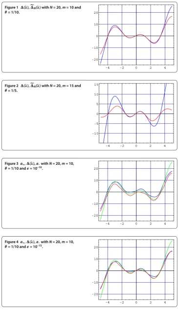
Figures and illustrate the comparison between(λ) andN(λ) for different values
inter-Figure 1 (λ),N(λ) withN= 20,m= 10 and θ= 1/10.
Figure 2 (λ),N(λ) withN= 20,m= 15 and θ= 1/5.
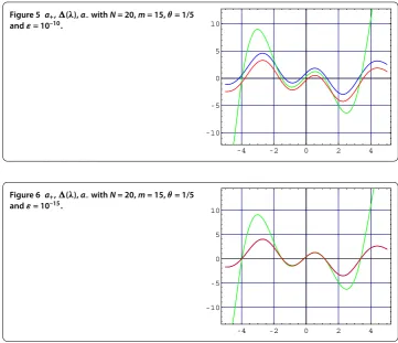
Figure 3 a+,(λ),a–withN= 20,m= 10,
θ= 1/10 andε= 10–10.
Figure 4 a+,(λ),a–withN= 20,m= 10,
Figure 5 a+,(λ),a–withN= 20,m= 15,θ= 1/5 andε= 10–10.
Figure 6 a+,(λ),a–withN= 20,m= 15,θ= 1/5 andε= 10–15.
vals forε= –andε= –, respectively. Also, Figures and illustrate the enclosure intervals forε= –andε= –, respectively, but form= ,θ= /.
Example The Dirac system
u(x) –xu(x) =λu(x), u(x) +xu(x) = –λu(x), ≤x≤, (.)
u() = , u() = –λu() (.)
is a special case of the problem treated in the previous section withr(x) =r(x) =x,
α=β= ,α=β=β= andβ= –. The characteristic function is
(λ) :=cos
+λ
–λsin
+λ
. (.)
The functionK(λ) will be
K(λ) :=cosλ–λsinλ. (.)
As in the previous example, Figures , , , , and illustrate the results of Tables , , , and . Figures and illustrate the comparison between(λ) andN(λ) for different
Figure 7 (λ),N(λ) withN= 20,m= 6 and θ= 1/14.
Figure 8 (λ),N(λ) withN= 20,m= 12 and θ= 1/8.
Figure 9 b+, (λ),b–withN= 20,m= 6,θ= 1/14 andε= 10–10.
Figure 10 b+, (λ),b–withN= 20,m= 6,
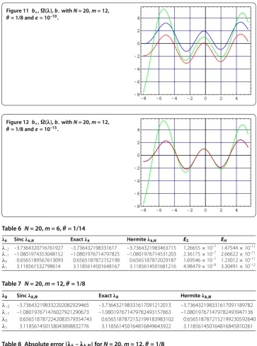
Figure 11 b+, (λ),b–withN= 20,m= 12,
θ= 1/8 andε= 10–10.
Figure 12 b+, (λ),b–withN= 20,m= 12,
θ= 1/8 andε= 10–15.
Table 6 N= 20,m= 6,θ= 1/14
λk Sincλk,N Exactλk Hermiteλk,N ES EH
λ–2 –3.7364320716761927 –3.736432198331617 –3.7364321983463715 1.26655×10⁻⁷ 1.47544×10⁻¹¹ λ–1 –1.0801974353048152 –1.0801976714797825 –1.0801976714531203 2.36175×10⁻⁷ 2.66622×10⁻¹¹ λ0 0.6565189567613093 0.6565187872152198 0.6565187872029187 1.69546×10⁻⁷ 1.23012×10⁻¹¹ λ1 3.118561532798614 3.1185614501648167 3.1185614501681216 4.98479×10⁻⁸ 3.30491×10⁻¹²
Table 7 N= 20,m= 12,θ= 1/8
λk Sincλk,N Exactλk Hermiteλk,N
λ–2 –3.736432198332202082929465 –3.736432198331617091212013 –3.736432198331617091189782
λ–1 –1.080197671476027921290673 –1.080197671479782493157863 –1.080197671479782493947136
λ0 0.6565187872242083579354743 0.6565187872152199183983102 0.6565187872152199230592640
λ1 3.118561450158043898832776 3.118561450164816849643922 3.118561450164816845810261
Table 8 Absolute error|λk–λk,N|forN= 20,m= 12,θ= 1/8
λk λ–2 λ–1 λ0 λ1
ES 5.849×10⁻¹³ 3.755×10⁻¹² 8.988×10⁻¹² 6.773×10⁻¹²
EH 2.223×10⁻²⁰ 7.893×10⁻¹⁹ 4.661×10⁻¹⁸ 3.834×10⁻¹⁸
Table 9 ForN= 20,m= 6 andθ= 1/14, the exact solutionsλkare all inside the interval
[b–,b+] for different values ofε
λk Exactλk [b–,b+],ε= 10–10 [b–,b+],ε= 10–15
λ–2 –3.736432198331617091212013 [–3.881037, –3.476447] [–3.836682, –3.557513]
λ–1 –1.080197671479782493157863 [–1.435432, –0.665868] [–1.365324, –0.760935]
λ0 0.6565187872152199183983102 [0.410872, 1.116247] [0.492155, 1.004381]
λ1 3.118561450164816849643922 [2.884061, 3.390359] [2.940901, 3.331955]
Table 10 WithN= 20,m= 12 andθ= 1/8,λkare all inside the interval [b–,b+] for different
values ofε
λk Exactλk [b–,b+],ε= 10–10 [b–,b+],ε= 10–15
λ–2 –3.736432198331617 [–4.1011429, –3.3717065] [–3.7364598, –3.7364045]
λ–1 –1.0801976714797825 [–1.5078873, –0.4433678] [–1.0808585, –1.07952734]
λ0 0.6565187872152198 [0.0168549, 1.1086918] [0.6528005, 0.6602210]
λ1 3.1185614501648167 [2.7401391, 3.1185614] [3.1157222, 3.1214041]
E10(Rθ,m) = 6.2724×10¹²,E9(Rθ,m) = 8.21004×10¹¹,ω= 1,MRθ,m= 501421.
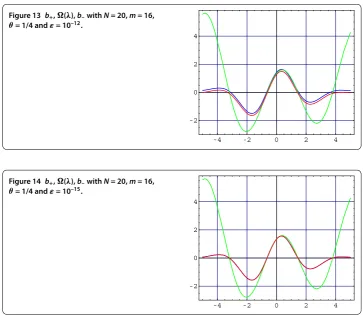
Figure 13 b+, (λ),b–withN= 20,m= 16,
θ= 1/4 andε= 10–12.
Figure 14 b+, (λ),b–withN= 20,m= 16,
θ= 1/4 andε= 10–15.
Table 11 N= 20,m= 16,θ= 1/4
λk Exactλk λk,N EH
λ–2 –3.1976270593385675784857858037 –3.1976270593385675784857498452 3.596×10⁻²³
λ–1 –0.64351783872891518984316280760 –0.64351783872891518984316309998 2.924×10⁻²⁵
λ0 1.4487204290456776077365351429 1.4487204290456776077365176362 1.751×10⁻²³
λ1 3.8015200831700579923508826075 3.8015200831700579923509045951 2.199×10⁻²³
Table 12 WithN= 20,m= 16 andθ= 1/4,λkare all inside the interval [b–,b+] for different
values ofε
λk Exactλk [b–,b+],ε= 10–10 [b–,b+],ε= 10–15
λ–2 –3.1976270593385675784857858037 [–3.30255437, –3.11013060] [–3.19791869, –3.19733846]
λ–1 –0.64351783872891518984316280760 [–0.67219637, –0.61489406] [–0.64356572, –0.64346999]
λ0 1.4487204290456776077365351429 [1.40795687, 1.49107473] [1.44812338, 1.44932224]
λ1 3.8015200831700579923508826075 [3.60636554, 4.19453907] [3.80103975, 3.80200804]
Example The boundary value problem
u(x) –xu(x) =λu(x), u(x) –u(x) = –λu(x), ≤x≤, (.)
u() = , u() =λu() (.)
is a special case of the problem(r,α,β, ,β) whenr(x) =x,r(x) = –,α=β=β = andα=β=β= . Here the characteristic function is
(λ) := /AiryAiPrimeλ( –λ)/AiryBiλ( –λ)/
–AiryAiλ( –λ)/AiryBiPrimeλ( –λ)/
×λ( –λ)/AiryAi( +λ)( –λ)/AiryBiλ( –λ)/
+AiryAiPrime(λ+ )( –λ)/AiryBiλ( –λ)/
–AiryAiPrimeλ( –λ)/λ( –λ)/AiryBi(λ+ )( –λ)/
+AiryBiPrime(λ+ )( –λ)/, (.)
where AiryAi[z] and AiryBi[z] are Airy functions Ai(z) and Bi(z), respectively, and
AiryAiPrime[z] andAiryBiPrime[z] are derivatives of Airy functions. The functionK(λ) will be
K(λ) :=cosλ–λsinλ. (.)
Figures , and Tables , illustrate the applications of the method to this problem.
Competing interests
The author declares that he has no competing interests.
Acknowledgements
This article was funded by the Deanship of Scientific Research (DSR), King Abdulaziz University, Jeddah. The author, therefore, acknowledges with thanks DSR technical and financial support.
Received: 8 November 2012 Accepted: 5 February 2013 Published: 21 February 2013
References
1. Grozev, GR, Rahman, QI: Reconstruction of entire functions from irregularly spaced sample points. Can. J. Math.48, 777-793 (1996)
2. Higgins, JR, Schmeisser, G, Voss, JJ: The sampling theorem and several equivalent results in analysis. J. Comput. Anal. Appl.2, 333-371 (2000)
3. Hinsen, G: Irregular sampling of bandlimitedLp-functions. J. Approx. Theory72, 346-364 (1993)
4. Jagerman, D, Fogel, L: Some general aspects of the sampling theorem. IRE Trans. Inf. Theory2, 139-146 (1956) 5. Annaby, MH, Asharabi, RM: Error analysis associated with uniform Hermite interpolations of bandlimited functions.
J. Korean Math. Soc.47, 1299-1316 (2010)
6. Higgins, JR: Sampling Theory in Fourier and Signal Analysis: Foundations. Oxford University Press, Oxford (1996) 7. Butzer, PL, Schmeisser, G, Stens, RL: An introduction to sampling analysis. In: Marvasti, F (ed.) Non Uniform Sampling:
Theory and Practices, pp. 17-121. Kluwer Academic, New York (2001)
8. Butzer, PL, Higgins, JR, Stens, RL: Sampling theory of signal analysis. In: Development of Mathematics 1950-2000, pp. 193-234. Birkhäuser, Basel (2000)
9. Annaby, MH, Asharabi, RM: On sinc-based method in computing eigenvalues of boundary-value problems. SIAM J. Numer. Anal.46, 671-690 (2008)
10. Annaby, MH, Tharwat, MM: On the computation of the eigenvalues of Dirac systems. Calcolo49, 221-240 (2012) 11. Annaby, MH, Tharwat, MM: On computing eigenvalues of second-order linear pencils. IMA J. Numer. Anal.27,
366-380 (2007)
13. Boumenir, A, Chanane, B: Eigenvalues of S-L systems using sampling theory. Appl. Anal.62, 323-334 (1996) 14. Tharwat, MM, Bhrawy, AH, Yildirim, A: Numerical computation of eigenvalues of discontinuous Sturm-Liouville
problems with parameter dependent boundary conditions using sinc method. Numer. Algorithms (2012). doi:10.1007/s11075-012-9609-3
15. Tharwat, MM, Bhrawy, AH, Yildirim, A: Numerical computation of eigenvalues of discontinuous Dirac system using sinc method with error analysis. Int. J. Comput. Math.89, 2061-2080 (2012)
16. Lund, J, Bowers, K: Sinc Methods for Quadrature and Differential Equations. SIAM, Philadelphia (1992) 17. Stenger, F: Numerical methods based on Whittaker cardinal, or sinc functions. SIAM Rev.23, 156-224 (1981) 18. Stenger, F: Numerical Methods Based on Sinc and Analytic Functions. Springer, New York (1993)
19. Butzer, PL, Splettstösser, W, Stens, RL: The sampling theorem and linear prediction in signal analysis. Jahresber. Dtsch. Math.-Ver.90, 1-70 (1988)
20. Jagerman, D: Bounds for truncation error of the sampling expansion. SIAM J. Appl. Math.14, 714-723 (1966) 21. Boas, RP: Entire Functions. Academic Press, New York (1954)
22. Levitan, BM, Sargsjan, IS: Introduction to Spectral Theory: Self Adjoint Ordinary Differential Operators. Translation of Mathematical Monographs, vol. 39. Am. Math. Soc., Providence (1975)
23. Levitan, BM, Sargsjan, IS: Sturm-Liouville and Dirac Operators. Kluwer Academic, Dordrecht (1991)
24. Annaby, MH, Tharwat, MM: The Hermite interpolation approach for computing eigenvalues of Dirac systems. Math. Comput. Model. (2012). doi:10.1016/j.mcm.2012.07.025
25. Kerimov, NB: A boundary value problem for the Dirac system with a spectral parameter in the boundary conditions. Differ. Equ.38, 164-174 (2002)
26. Annaby, MH, Tharwat, MM: On sampling and Dirac systems with eigenparameter in the boundary conditions. J. Appl. Math. Comput.36, 291-317 (2011)
27. Boumenir, A: Higher approximation of eigenvalues by the sampling method. BIT Numer. Math.40, 215-225 (2000) 28. Tharwat, MM, Bhrawy, AH: Computation of eigenvalues of discontinuous Dirac system using Hermite interpolation
technique. Adv. Differ. Equ. (2012). doi:10.1186/1687-1847-2012-59
doi:10.1186/1687-2770-2013-36
![Table 5 With Nvalues of = 20, m = 15 and θ = 1/5, λk are all inside the interval [a–,a+] for different ε](https://thumb-us.123doks.com/thumbv2/123dok_us/483645.2047236/14.595.117.481.478.535/table-nvalues-th-lk-inside-interval-different-e.webp)