A Framework for Identifying Compromised Nodes in
Sensor Networks
Qing Zhang Ting Yu Peng Ning
Department of Computer Science North Carolina State University {qzhang4, tyu, pning}@ncsu.edu
Abstract
Sensor networks are often deployed in open environments. They are vulnerable to physical attacks. Once a node’s cryptographic key is compromised, an attacker may completely im-personate it, and introduce arbitrary false information into the network. Basic cryptographic security mechanisms are often not effective in this situation. Most techniques to address this problem focus on detecting and tolerating false information introduced by compromised nodes. They cannot pinpoint exactly where the false information is introduced and who is responsible for it. We still lack effective techniques to accuratelyidentifycompromised nodes so that they can be excluded from a sensor network once and for all.
This paper proposes an application-independent framework for identifying compromised sen-sor nodes. In this framework, sensen-sor nodes may conceptually observe the activity of each other following the deployment topology of a sensor network. An alert is generated if a node observes an abnormal activity. Such alerts are collected by the base station, which further reason and finally identify compromised nodes. The reasoning process is very challenging due to the fact that compromised nodes may very well raise false alerts. They may also form local majorities and collude to further mislead the base station. In this paper, we develop efficient and accurate reasoning algorithms that can effectively deal with collusion and local majorities. Our algo-rithms are optimal in the sense that they identify the largest number of compromised nodes without introducing false positives. We evaluate the effectiveness of our algorithms through comprehensive experiments.
1
Introduction
Low-power wireless sensor networks can be rapidly deployed in a large geographical area in a self-configured manner. This makes them particularly suitable for real-time, large-scale information collection and event monitoring for mission-critical applications in hostile environments, such as target tracking and battlefield surveillance.
Such applications, meanwhile, impose unique security challenges. In particular, since sensors are often deployed in open environments, they are vulnerable to physical attacks. Once recovering the keying materials of some nodes, an adversary is able to impersonate them completely, and inject arbitrary false information. Basic cryptographic security mechanisms, such as authentication and integrity protection, are often not effective against such impersonation attacks [6].
Recently, several approaches have been proposed to cope with compromised nodes, which mainly fall into two categories. Approaches in the first category are to detect and tolerate false information introduced by attackers [5, 10, 22], in particular during data aggregation. Once the base station receives aggregated data, it checks their validity through mechanisms such as sampling and the deployment of redundant sensors. However, these techniques cannot be used to identify exactly where the false information is introduced and who is responsible for it.
Approaches in the second category rely on application specific detection mechanisms which en-able sensor nodes to monitor the activities of others nearby. Once an abnormal activity is observed, a node may raise an alert either to the base station or to other nodes, who further determine which nodes are compromised. We call approaches in this categoryalert-based. Representative alert-based approaches include those in sensor network routing [8] and localization [16].
be trusted since compromised nodes may also raise false alerts to mislead the base station and other nodes. Compromised nodes may further form a local majority and collude, increasing their influences in the network. Further, existing alert-based approaches are application specific. They cannot be easily extended to other domains. A general solution to the accurate identification of compromised nodes still remains elusive.
The problem of false alerts (or feedback) and collusion also arises in other decentralized systems such as online auction communities and P2P systems [1, 11, 13, 19, 23, 25, 26]. Reputation-based trust management has been adopted as an effective means to form cooperative groups in the above systems. One seemingly attractive approach is to apply existing trust management techniques in sensor networks. For example, we may identify sensor nodes with the lowest trust values as compromised. However, as a decentralized system, sensor networks bear quite unique properties. Many assumptions in reputation-based trust management do not hold in sensor networks. Thus, simply applying those techniques is unlikely to be effective (see section 4 for a detailed experimental comparison).
For example, in P2P systems, interactions may happen between any two entities. If an entity provides misleading information or poor services, it is likely that some other entities will be able to detect it and issue negative feedback accordingly. The interactions among sensor nodes, however, are restricted by the deployment of a sensor network. For a given node, only a fixed set of nodes are able to observe it. Thus, it is easy for compromised nodes to form local majorities.
Also, most decentralized systems are composed of autonomous entities, which pursue to maxi-mize its own interests. Incentive mechanisms are needed to encourage entities to issue (or at least not discourage them from issuing) feedback about others. A sensor network, on the other hand, is essentially a distributed system. Sensor nodes are designed to cooperate and finish a common task. Therefore, it is possible to design identification mechanisms that achieve global optimality for a given goal. For instance, to cope with false alerts, we may choose to identify as compromised both the target and the issuer of an alert, as long as it will improve the security of the whole system. Such an approach is usually not acceptable in P2P systems and online auction communities.
Indeed, the unique properties of sensor networks bring both challenges and opportunities. How to accommodate and take advantages of these properties is the key to the accurate identification of compromised nodes.
In this paper, we propose novel techniques to provide general solutions to the identification of compromised sensor nodes. Our techniques are based on an application-independent framework that abstracts some of the unique and intrinsic properties of sensor networks. It can be used to model a large range of existing sensor network applications. In summary, our contributions include the following:
1. We generalize the model of alert-based approaches, and propose an application-independent framework for identifying compromised nodes. The central component of the framework is an abstraction of the monitoring relationship between sensor nodes. Such relationship can be derived from application specific detection mechanisms. The framework further models sensor nodes’ sensing and monitoring capabilities, and their impacts on detection accuracy. We show by example that many existing sensor networks can be easily modeled by the proposed framework.
2. Based on the proposed framework, we design efficient algorithms to accurately identify com-promised sensor nodes for situations where (1) comcom-promised nodes inject false information and false alerts independently, and (2) compromised nodes form local majorities and collude to inject false information and false alerts. We show that our algorithms are optimal, in the sense that they identify the largest number of compromised nodes without introducing any false positives. We also propose techniques to further eliminate those compromised nodes that cannot be directly identified by the above algorithms. To the best of our knowledge, our work is the first application-independent approach to identifying compromised sensor nodes. 3. We conduct comprehensive experiments to evaluate the proposed techniques. The results
B1
B2
B3
B4
B5
B6 S2
S3
S4
S6
S5
S7
S1
(a) The deployment of beacon nodes in sen-sor network localization
B6 B5
B4
B3 B2
B1
(b) The observability graph of sensor network localization
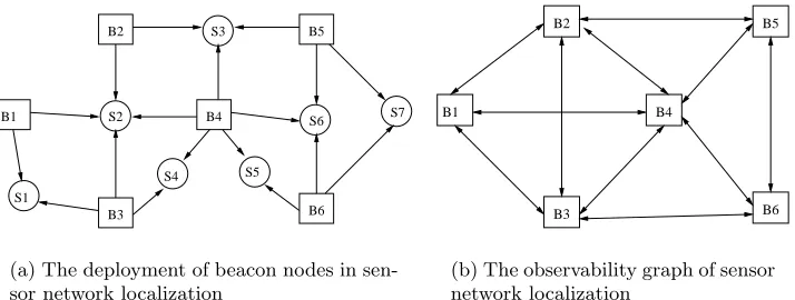
Figure 1: An example deployment of sensor nodes in sensor network localization and its corre-sponding observability graphs
The rest of the paper is organized as follows. Section 2 presents a general framework for identifying compromised nodes, and shows how sensor network application can be modeled by the framework. In section 3, we present algorithms that identify compromised sensor nodes for both the collusion and non-collusion cases. In section 4, we show the effectiveness of our algorithms through experimental evaluation. Some relevant issues are discussed in section 5. Section 6 reports closed related work. Concluding remarks are given in section 7.
2
A General Framework for Identifying Compromised Nodes
In this section, we first use an example to identify the aspects of sensor networks that are relevant to the identification of compromised nodes. We then present the general framework.
2.1 An Example Sensor Network Application
Many sensor network applications require sensors’ location information (e.g., in target tracking). Since it is often too expensive to equip localization devices such as GPS receivers on every node, many location discovery algorithms depend on beacon nodes, i.e., sensor nodes aware of their locations. A non-beacon node queries beacon nodes nearby for references, and estimates its own location. An example deployment of the sensor network is shown in figure 1(a), where beacon nodes and non-beacon nodes are represented by rectangle and round nodes respectively. An edge from a beacon node bto a non-beacon nodesindicates that bcan provide location references to s.
A compromised beacon node may claim its own location arbitrarily, making non-beacon nodes around derive their locations incorrectly. Liu et al. [16] proposed a mechanism to detect malicious beacon nodes. The basic idea is to let beacon nodes probe each other and check the sanity of the claimed locations. Suppose beacon node b1’s location is (x, y) and beacon node b2 claims its
location to be (x, y). If the difference between the derived distance and the measured distance exceeds a threshold , then b1 will consider b2 as compromised, and report to the base station.
Clearly, a compromised beacon node may also send false alerts to the base station.
After receiving a set of alerts from beacon nodes, what information is needed for the base station to make a rational decision on compromised nodes? First, the base station has to know whether an alert is valid, i.e., whether beacon nodesb1 and b2 are close enough to probe each other. In other
words, the monitoring relationship between beacon nodes is needed.
Second, due to the imprecision of distance measuring, it is possible that an alert is raised by an uncompromised beacon node against another uncompromised one. The base station has to take this possibility into consideration.
Third, it is necessary to regularly probe a beacon node so that it can be detected promptly if that beacon node is compromised and provides misleading location references.
2.2 Assumptions
We make the following assumptions about sensor network applications before presenting a general framework for identifying compromised nodes.
First, we assume there exist application-specific detection mechanisms deployed in a sensor net-work, which enable sensor nodes to observe each other’s activities. Such detection mechanisms are commonly employed in sensor networks. Examples include beacon node probing in sensor network localization as mentioned above, witnesses in data aggregation [5] and the watchdog mechanism [8]. A sensor nodes1 is called anobserverof another nodes2 ifs1 can observe the activities of s2.
A node may have multiple observers or observe multiple other nodes.
Second, we focus on static sensor networks, where sensor nodes do not change their locations dramatically once deployed. A large range of sensor networks fall into this category. One con-sequence of this assumption is that the observability relationship between sensor nodes does not change unless a sensor network is reconfigured.
Third, we assume that message confidentiality and integrity are protected through key manage-ment and authentication mechanisms [4, 7, 9].
Finally, we assume the base station of a sensor network is trusted, and has sufficient computation and communication capabilities. Hence, we adopt a centralized approach, where the base station is responsible for reasoning about the alerts and identifying compromised nodes. The responsibility of each node is only to observe abnormal activities and raise alerts to the base station. We briefly discuss in section 5 decentralized approaches, where sensor nodes also take part in the reasoning and identification process.
2.3 The Framework
With the above assumptions, our framework for identifying compromised nodes is composed of the following components:
Observability graph. An observability graph is a directed graph G(V, E), where V is a set of vertices that represent sensor nodes, andE is a set of edges. An edge (s1, s2)∈E if and only
if s1 is an observer of s2. An observability graph is derived from the detection mechanism
of an application. Note that V only contains those nodes whose security is concerned by a detection mechanism. For example, in sensor network localization, the observability graph only includes beacon nodes. Figure 1(b) shows the observability graph corresponding to the sensor network localization deployment in figure 1(a).
Alerts. An alert takes the form (t, s1, s2), indicating that nodes1 observes an abnormal activity of
s2 at timet. The information in an alert may be further enriched, for example, by including
s1’s confidence on the alert. For simplicity, this paper omits such parameters. Note that
alerts may not need to be explicitly sent by sensor nodes. Instead, in some applications they may be implicitly inferred by the base station from application data sent by sensor nodes. Sensor behavior model. Sensors are not perfect. Even if a node is uncompromised, it may still
occasionally report inaccurate information or behave abnormally. A sensor behavior model includes a parameter rm (called the reliability of sensors) which represents the percentage
of normal activities conducted by an uncompromised node. For example, in sensor network localization, if rm = 0.99, then 99% of the time, an uncompromised beacon node provides
correct location references.
Observer model. Similarly, an observer model represents the effectiveness of the detection mech-anism of a sensor network, which is captured by itsobservability rate rb,positive accuracyrp
and negative accuracyrn. rb is the probability that an observers1 observes an activity when
it is conducted by an observee s2. This reflects the fact that in some applications, due to
cost and energy concerns, s1 may not observe every activity of s2. The positive accuracyrp
is the probability that s1 raises an alert when s2 conducts an abnormal activity observed by
s1. Similarly,rn is the probability thats1 does not raise an alert when s2 conducts a normal
activity observed by s1. rp and rn reflect the intrinsic capability of a detection mechanism.
Security estimation. If it is possible that all the nodes in the network are compromised, then in general the base station cannot identify definitely which nodes are compromised based on alerts. Therefore, this framework focuses on the situation where the number of compromised nodes does not exceed a certain threshold K. This threshold is application specific. We call
K thesecurity estimationof a network. We emphasize thatK is only anupper boundof the
number of compromised nodes. The base station does not need to know the exact number of compromised nodes in a network.
Identification function. An identification function F determines which nodes are compromised. Formally, it takes as inputs the observability graph G, the sensor reliabilityrm, the observer
model (rb, rp, rn), the security estimationK, and a set of alerts raised during a periodT, and
returns a set of node IDs, which indicate those nodes that are considered compromised.
The above framework is application independent. It can be used to model a large range of sensor networks. In appendix A, we use two examples (sensor network localization [16] described in section 2.1 and a sensor network data fusion application [5]) to show the applicability of the proposed framework. Note that in the appendix we intentionally omit the discussion of identification functions when modeling the above applications, since neither work [5, 16] handles false alerts from compromised nodes. Though inconsistencies between alerts may be discovered, no solution is provided to reason which nodes are compromised.
3
Identification of Compromised Nodes
In this section, we present our approaches to identifying compromised sensor nodes based on the above framework
Let s1 be an observer of s2. Intuitively, if s1 raises an alert against s2, then at least one of
them is compromised. Otherwise, if both behave normally, there should be no alerts between them. However, sensors are not assumed to have perfect sensing and monitoring capabilities. Thus, the base station cannot draw any definite conclusion from a single alert. Instead, it needs to observe the alert pattern during a certain period of time to discover suspicious activities with high confidence. Given a network’s sensor behavior model, its observer model and the frequency of the monitored events, we can derive the expected number of alerts raised bys1 againsts2 during a period of time,
when they are uncompromised. During the operation of the sensor network, the base station compares the number of alerts actually raised by s1 against s2 with the expected number. Only
when the former is higher than the latter with statistical significance, should the base station consider it as abnormal. Specifically, for every event sensed by a node sj, the probability that si
raises an alert against sj is given by C = rb ·((rm ·(1−rn) + (1−rm)·rp). Let fj(x) be the
distribution of events that can be sensed by sj. Then the distribution of alerts along the edge
(si, sj) (i.e., those raised bysi againstsj) is fij(x) =fj(Cx). For a period t, the expected number
of alerts along (si, sj) will beRij(t) =C t
fij(x).
During a time period T, if the number of alerts along the edge (si, sj) is over Ri,j(|T|) +δ,
whereδ ≥0 is an application specific parameter, then we say the edge (si, sj) is an abnormal edge
in the observability graph. Otherwise, (si, sj) isnormal. An abnormal edge can be interpreted as a
definite claim fromsi thatsj is compromised. Similarly, a normal edge representssi’s endorsement
thatsj is not compromised.
Given an abnormal edge (si, sj), eithersi is compromised and raises many bogus alerts against
sj, orsj is compromised and its malicious activities are observed bysi, or both. Further suppose
there is an additional normal edge (sl, sj). Then one ofsi andslmust be compromised. Otherwise,
the two edges should be consistent with each other sinceslandsiobserve the activities of the same
node sj during the same period of time.
Definition 3.1. Given an observability graphG(V, E), letEa andEn be the set of abnormal edges
and normal edges inGrespectively. We say that two sensor nodes si andsj form a suspicious pair
if one of the following holds: 1. (si, sj)∈Ea or (sj, si)∈Ea;
2. There exists a sensor node s, such that either (si, s)∈Ea and(sj, s)∈En, or (si, s)∈En
1 2
6 5
7 8 9
4
3 1 3
4 5
7 8
2
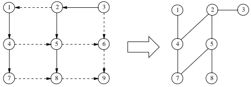
Figure 2: An observability graph and its corresponding inferred graph
Let {s1, s1}, ...,{sk, sk} be the suspicious pairs derived from an observability graphG. The inferred
graph of G is an undirected graph I(V, E) such thatV =1≤i≤k{si, si} and E ={{si, si} |1≤
i≤k}.
Intutively, if (si, sj) are a suspicious pair, then at least one of them is compromised. Note that
if a pair of node is not suspicious, it does not mean that they are both uncompromised. It only means we cannot infer anything about them.
The left part of figure 3 shows an observability graph, where abnormal and normal edges are represented by solid and dashed edges respectively. The corresponding inferred graph is shown in the right part of the figure. Note that an inferred graph may not be connected.
From the figure one may wonder that, since (2,1) is normal and (2,5) is abnormal, shouldn’t
{1,5} be a suspicious pair? The answer is no since it is possible that node 2 is compromised, and selectively issues bogus alerts against node 1 but not node 5, even though both node 1 and 5 are uncompromised. Similarly, a compromised node may sense data normally but issue bogus alerts or vise versa. So{1,3}is not a suspicious pair even though (3,2) is abnormal and (2,1) is normal. In other words, transitivity does not hold when constructing suspicious pairs.
Clearly, if a sensor node does not appear in the inferred graph, then its behavior is consistent with the sensor behavior model and observer model, and thus should be considered uncompro-mised. Hence, we concentrate on identifying compromised sensor nodes among those involved in the inferred graph.
Definition 3.2. Given an inferred graph I(V, E) and a security estimationK, a valid assignment
with regard toI andK is a pair(Sg, Sb), whereSg andSb are two sets of sensor nodes that satisfies
all of the following conditions:
1. Sg and Sb is a partition of V, i.e., Sg∪Sb =V and Sg∩Sb =∅;
2. For any two sensor nodes si and sj, if si∈Sg and sj ∈Sg, then {si, sj} ∈E; and
3. |Sb| ≤K.
Intuitively, a valid assignment corresponds to one possible way that sensor nodes are compro-mised, so that, when they raise false alerts and conduct abnormal activities, the resulting inferred graph isI. Sg and Sb contains the uncompromised and compromised nodes respectively. Given an
inferred graph and a security estimationK, there may exist many valid assignments. If a nodes
is included in theSb of every possible valid assignment, then we are sure thats is compromised.
Definition 3.3. Given an inferred graph I(V, E) and a security estimation K, let {(Sg1, Sb1),
. . . ,(Sgn, Sbn)}be the set of all the valid assignments with regard toI andK. We call
1≤i≤nSbithe
compromised coreof the inferred graphIwith security estimationK, denotedCompromisedCore(I, K).
Similarly, 1≤i≤nSgi is called the uncompromised core of I with security estimation K, denoted
U ncompromisedCore(I, K).
If an identification function always returns the compromised core of an inferred graph I with security estimationK, then the function isoptimalin the sense that it identifies the largest number of compromised nodes without introducing any false positives. Thus, given the general framework,
On the other hand, though introducing no false positives, the compromised core may not achieve high detection rates since there may exist suspicious pairs whose nodes are not included in the com-promised core. Thus,another key problem is to seek techniques that further eliminate compromised
nodes without causing many false positives.
In summary, our approach is composed of two phases. In the first phase, we compute or approximate the compromised core, identifying those nodes that are definitely compromised. In the second phase, we tradeoff accuracy for eliminating more compromised nodes.
3.1 Identification of Colluding Compromised Sensor Nodes
Let us first consider a special case in which there is no edge between two compromised sensor nodes in the inferred graph. This corresponds to a strong collusion model where compromised nodes are well coordinated so that they do not raise alerts against each other, and alerts against a node from two compromised nodes are consistent. It is easy to see that in this case the inferred graph is bipartite. We call inferred graphs in this situation collusion-inferred graphs.
Let G1, . . . , Gz be the connected components of a collusion inferred graph I. For each Gi,
1≤i≤z, let Ai, Bi denote the two sets of disjoint vertices inGi such that vertices in one set are
adjacent only to vertices in the other set. We call (Ai, Bi) thetwo-color partitionofGi. Without loss
of generality, we assume|Ai| ≥ |Bi|. Clearly, since I is collusion inferred, vertices in the same set
are either all compromised or all uncompromised. Further, if vertices in one set are compromised (uncompromised), then vertices in the other set are uncompromised (compromised). Therefore,
1≤i≤z|Bi|gives a lower bound of the number of compromised nodes in a network.
Lemma 3.1. Let I(V, E) be a collusion-inferred graph andK be a security estimation. Given the
two-color partition (Ai, Bi) of any connected component of I, 1≤i≤z, let Qi be either Ai or Bi.
We haveQi ⊆U ncompromisedCore(I, K) if and only if |Qi|+
j=i|Bj|> K.
Intuitively, ifQiis compromised, then|Qi|+
j=i|Bi|gives a tighter lower bound of the number
of compromised nodes, which should be no more thanK.
Corollary 3.1. Given any connected component Gi of a collusion inferred graphI, and a security
estimation K, Bi⊆U ncompromisedCore(G, K).
Theorem 3.1. Given a collusion inferred graph I with z connected components, and a
secu-rity estimation K, let (Ai, Bi), 1 ≤ i ≤ z, be the two-color partition of each connected
compo-nent. Let Sb = {Bi | |Ai|+
j=i|Bj| > K}, and Sa = {Ai | |Ai|+
j=i|Bj| > K}. Then
CompromisedCore(I, K) =Bi∈S
bBi and U ncompromisedCore(I, K) =
Ai∈SaAi.
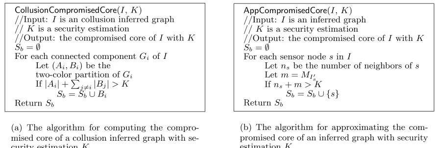
Given theorem 3.1, it is straightforward to develop the algorithm that efficiently compute
CompromisedCore(I, K). The pseudocode of the algorithm is shown in figure 3(a).
Theorem 3.2. The complexity of algorithm CollusionCompromisedCore is O(n+m), where n and
m are the numbers of vertices and edges respectively in an collusion inferred graph.
3.2 A General Algorithm to Identify Compromised Sensor Nodes
The discussion above has made two assumptions. First, we assume that compromised nodes follow a strong collusion model, so that no suspicious pair contains two compromised nodes. Second, we assume that the base station is aware of the collusion. The effectiveness of the algorithm shown in figure 3(a) relies on the fact that compromised nodes always collude.
When compromised nodes do not follow the collusion model strictly, the inferred graph may not be bipartite any more, and thus the above algorithm cannot be applied. Note that, even if an inferred graph is bipartite, it does not necessarily mean that compromised nodes are colluding. For example, suppose the inferred graph contains two suspicious pairs{s1, s2} and{s1, s3}. Though it
is bipartite, it is possible that boths1 ands2 are compromised, but raise alerts against each other.
CollusionCompromisedCore(I,K) //Input: Iis an collusion inferred graph //Kis a security estimation
//Output: the compromised core ofI withK Sb=∅
For each connected componentGi ofI
Let (Ai, Bi) be the
two-color partition ofGi
If|Ai|+
j=i|Bj|> K
Sb=Sb∪Bi
ReturnSb
(a) The algorithm for computing the compro-mised core of a collusion inferred graph with se-curity estimationK
AppCompromisedCore(I,K) //Input: I is an inferred graph //K is a security estimation
//Output: the compromised core ofI withK Sb=∅
For each sensor nodesinI
Letns be the number of neighbors ofs
Letm=MIs
Ifns+m > K
Sb=Sb∪ {s}
ReturnSb
(b) The algorithm for approximating the com-promised core of an inferred graph with security estimationK
Figure 3: Efficient algorithms for computing the compromised core
Lemma 3.2. Given an inferred graph I(V, E), let VI be a minimum vertex cover of I. Then the
number of compromised nodes is no less than |VI|.
We denote the size of the minimum vertex covers of an undirected graph G as CG. Given a
sensor nodes, the neighbors of sin an inferred graph I is denoted Ns. Further, let Is denote the
graph after removing s and its neighbors from I. We have the following theorem for identifying compromised sensor nodes.
Theorem 3.3. Given an inferred graph I and a security estimation K, for any node s in I,
s∈CompromisedCore(I, K) if and only if |Ns|+CIs > K.
Intuitively, if we assume a sensor node sis uncompromised, then all its neighbors inI must be compromised. According to lemma 3.2, there are at least |Ns|+CIs compromised nodes, which
should be no more than the security estimationK. Otherwise,smust be compromised. Meanwhile, if|Ns|+CIs ≤K, we can always construct a valid assignment for I with regard to K, where sis
assigned as uncompromised, which means sis not inCompromsedCore(I, K).
By theorem 3.3, the algorithm to identifyCompromisedCore(I, K) is straightforward. For each nodes, we check whether |Ns|+CIs is larger thanK. Unfortunately, this algorithm is in general
not efficient since the minimum vertex covering problem is NP-complete. In theory we also have to compute the minimum vertex cover of a different graph when checking each node.
Thus, we seek efficient algorithms to approximate the size of minimum vertex covers. To prevent false positives, we are interested in a goodlower boundof the size of minimum vertex covers, a goal different from that of many existing approximation algorithms. In this paper, we choose the size of maximum matchings of I as such an approximate. We denote the size of the maximum matchings of an undirected graph GasMG.
Lemma 3.3. Given an undirected graph G, MG≤CG≤2MG. And the bounds are tight.
Corollary 3.2. Given an inferred graph I and a security estimation K, for any node s in I, if |Ns|+MIs > K, then s∈CompromisedCore(I, K).
A maximum matching of an undirected graph can be computed in polynomial time [18]. Figure 3(b) shows an efficient algorithm to approximate the compromised core. Since this algorithm does not assume any specific collusion model among compromised nodes, we call it the general
identification algorithm, and the one in section 3.1 the bipartite identification algorithm.
Theorem 3.4. The complexity of the algorithm AppCompromisedCore is O(mn√n), where m is
3.3 Further Elimination of Compromised Sensor Nodes
The above algorithms do not introduce any false positives. Compromised nodes identified by the above algorithms may be safely excluded from the networks through, e.g., key revocation [4, 15]. However, there may still be suspicious pairs left that do no include any nodes in the compromised core. We call the graph composed of such pairs theresidual graph.
We may tradeoff accuracy for eliminating more compromised nodes. Since a suspicious pair contains at least one compromised node, identifying both nodes as compromised will introduce at most one false positive. By computing the maximum matching of a residual graph and treating them as compromised, the false positive rate is bounded by 0.5.
Therefore, given an inferred graph, we first compute or approximate its compromised core. We then compute the maximum matching of the residual graph, and further eliminate compromised nodes.
4
Experiments
We simulate a sensor network deployed to monitor the temperature of an area of 100m×100m. For simplicity, we assume sensor nodes are randomly distributed in the area. We adopt a simple detection mechanism. If the distance between two sensor nodes is within 10 meters, and the temperatures reported by them differ by more than 1◦C, the base station infers that each of them raises an alert against the other. In other words, two nodes are observers of each other if they are with in 10 meters. We assume that, once a network is deployed, sensors’ location information can be collected through localization techniques. Therefore, the base station is able to construct an observability graph accordingly.
Sensor nodes report temperatures to the base station once per minute, and the sensed data follows a normal distributionN(µ, σ2), whereµis the true temperature at a location, andσ= 0.2, which is consistent with the accuracy of typical thermistors in sensor network [24].
Unless otherwise stated, we assume 10% ∼15% of the nodes in the network are compromised. The security estimation is K = 0.15N, where N is the total number of nodes in the network. The goal of the attacker is to raise the temperature reading in the area. The attacker may choose to either randomly compromise nodes in the field, in which case no local majority is formed, or to compromise nodes centered around a position (x, y), following a normal distribution with a standard deviation σd. The latter corresponds to the case of local majority, and the parameter σd
controls its strength. The smaller σd is, the closer compromised nodes are to each other, and thus
the stronger the local majority is. We call σd theconcentrationof compromised nodes.
The evaluation metrics of the experiments are the detection rates and false positive rates of the proposed identification approaches.
We act conservatively, and assume that compromised nodes are in fact colluding, but the base station has to use the general detection algorithm since it cannot assume so. Thus, in the exper-iments, compromised nodes always collude. We then compare the effectiveness of the following approaches: (1) bipartite+mm: the bipartite identification algorithm followed by the maximum matching approach; (2)bipartite-only: the bipartite identification algorithm alone; (3)general+mm: the general identification algorithm followed by the maximum matching approach; and (4) general-only: the general identification algorithm alone. The comparision helps us investigate how much benefits it will bring if the base station is aware of the collusion among compromised nodes.
We further compare our approaches with EigenRep [11], a well-known reputation-based trust management scheme for P2P systems. The idea of EigenRep is similar to the PageRank algorithm [12]. In EigenRep, the number of satisfactory and unsatisfactory transactions between each pair of entities is collected to construct a matrix. One special property of the matrix is that the entries in each row add up to 1. The matrix is repetitively multiplied with an initial vector until it converges. The initial vector is a pre-defined parameter that corresponds to the default trust value of each entity. Each entry in the converged vector represents an entity’s final trust value. Since the trust values of all nodes always add up to 1, 1/N is the average trust value of sensor nodes in the network. In the experiment, we identify the K nodes with the lowest trust values as compromised, unless their trust values are over 1/N.
0 0.1 0.2 0.3 0.4 0.5 0.6 0.7 0.8 0.9 1
50 75 100 125 150 175 200 225 250
Number of sensors in a network
Detection rate
bipartite+mm bipartite-only general+mm general-only EigenRep
0 0.1 0.2 0.3 0.4 0.5 0.6 0.7
50 75 100 125 150 175 200 225 250
Number of sensors in a network
False positive rate
bipartite+mm bipartite-only general+mm general-only EigenRep
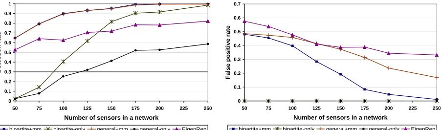
Figure 4: The impact of the deployment density of sensor nodes
from 50 to 250. The concentration of compromised nodes is set to be 20. Figure 4(a) and 4(b) show respectively the detection rate and false positive rate of each approach.
We see that when the number of sensor nodes increases, all the approaches achieve better detection rates and less false positive rates. Intuitively, the more densely sensor nodes are deployed, the more observers each node has, and thus the more likely an abnormal activity is detected. Another observation is that, bipartite+mm and general+mm achieve almost the same detection rates. However, the false positive rate of the latter is much higher than that of the former, since the latter takes advantages of the fact that compromised nodes are colluding, which helps identify compromised nodes more accurately. The third observation is that using the bipartite and the general identification algorithms alone do not achieve high detection rates when sensor nodes are deployed very loosely. This is because there are very few alerts for the base station to identify compromised nodes definitely. Note that these are the best that the base station can do without introducing false positives. Finally, we see that thebipartite+mmand the general+mmapproaches can detect much more compromised nodes with much fewer false positives than EigenRep, due to the fact that they take the unique properties of sensor networks into consideration, instead of treating it as a generic decentralized system.
Local majority. Figure 5 shows the effectiveness of different approaches when compromised nodes form local majorities. The number of nodes in the network is set to be 200. The concentration of compromised nodes is varied from 5 to 200. When compromised nodes are extremely close to each other, they essentially form a cluster. Suspicious pairs only involve those compromised nodes near the edge of the cluster. Those near the center of the cluster do not appear in the inferred graph, and thus cannot be identified. However, even at this situation, thebipartite+mmand general+mm
approaches can still achieve detection rate over 0.6, mainly due to the maximum matching approach in the second phase. When the compromised nodes are less concentrated, the bipartite and the general algorithms enables the base station to quickly identify almost all the compromised nodes. That is why we see a quick rise in their detection rates and a sharp drop in their false positive rates. Again, we observe that EigenRep is inferior to bothbipartite+mmand general+mm.
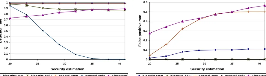
Accuracy of the security estimation. The security estimation is an important parameter for identification functions to infer compromised nodes. An accurate security estimation is not expected to always be available. The next experiment evaluate how the accuracy of a security estimation affects the effectiveness of different approaches. The total number of sensor nodes are set to 200. The number of compromised nodes and their concentration are both set to 20. The security estimation is varied from 20 to 40. The smaller the security estimation is, the more accurate it is. The experiment results are shown in figure 6.
0 0.1 0.2 0.3 0.4 0.5 0.6 0.7 0.8 0.9 1
0 20 40 60 80 100 120 140 160 180 200
Concentration of compromised sensors
Detection rate
bipartite+mm bipartite-only general+mm general-only EigenRep
0 0.1 0.2 0.3 0.4 0.5 0.6
0 20 40 60 80 100 120 140 160 180 200
Concentration of compromised nodes
False positive rate
bipartite+mm bipartite-only general+mm general-only EigenRep
Figure 5: The impact of the concentration of compromised sensor nodes
0 0.1 0.2 0.3 0.4 0.5 0.6 0.7 0.8 0.9 1
20 25 30 35 40
Security estimation
Detection rate
bipartite+mm bipartite-only general+mm general-only EigenRep
0 0.1 0.2 0.3 0.4 0.5 0.6
20 25 30 35 40
Security estimation
False positive rate
bipartite+mm bipartite-only general+mm general-only EigenRep
Figure 6: The impact of the accuracy of security estimation
matching approach. That explains why the false positives increase while detection rates remain high. The detection rate of EigenRep in fact improves when the security estimation accuracy decreases. This is because EigenRep always chooses the K nodes with lowest trust values, which will include more compromised nodes. But it also dramatically increases its false positive rate.
In summary, our experiments show that the two-phase approaches can always achieve very high detection rates with low false positives, even when sensor nodes are relatively loosely deployed, and compromised nodes form strong local majorities. Also, since they are designed to accommodate the uniqueness of sensor networks, they consistently outperform EigenRep, a reputation-based trust management schemes for general decentralized systems. Further, though the bipartite-only and
general-only approaches cannot achieve as high detection rates as bipartite+mm and general+mm, they do not introduce any false positives, which may be a desirable property for many applications.
5
Discussion
Attacks The proposed framework and algorithms focus on identifying compromised nodes through reasoning about alerts between sensor nodes. One possible attack is that an attacker may repetitively trigger events that can only be monitored by a nodes. Thus, the data reported by s may be significantly different from that of others. This may cause many alerts against
s, and have s identified as compromised. The essential reason for such attack is that the detection mechanism cannot tell the difference of information of a real phenomenon from pure bogus information generated by a compromised node. This problem cannot be handled by the general framework. Instead, it requires more accurate application detection mechanisms, e.g., having sensor nodes more densely deployed so that any event can be monitored by multiple nodes.
collects alerts and identifies potentially compromised nodes. A centralized approach usually offers better accuracy in identifying compromised and malfunctional nodes, since it has a global view of the network. A decentralized approach (as in [8]) is a possible alternative, which limits alerts to be exchanged between nearby nodes. A decentralized approach may incur less communication costs and be more scalable in some applications1. But without global information, it is in general more difficult to deal with the local majority and collusion of compromised nodes. How to design light-weighted decentralized approach to accurately identify compromised nodes is a challenging problem.
6
Related Work
Much work has been done to provide security primitives for wireless sensor networks, including practical key management [2, 4, 7, 15], broadcast authentication [14, 20, 21], and data authentication [10, 22, 27] as well as secure in-network processing [3]. The work of this paper is complementary to the above techniques, and can be combined to achieve high information assurance for sensor network applications. Several approaches have been proposed to detect and tolerate false information from compromised sensor nodes [5, 10, 22] through e.g., sampling and redundancy. But they do not provide mechanisms to accurately identify compromised sensor nodes, which is the focus of this paper.
Reputation-based trust management has been studied in different application contexts, includ-ing P2P systems, wireless ad hoc networks, social networks and the Semantic Web [1, 11, 13, 19, 23]. Many trust inference schemes have been proposed. They different greatly in inference methodolo-gies, complexity and accuracy. As discussed early, the interaction model and assumptions in the above applications are different from sensor networks. Directly applying existing trust inference schemes may not yield satisfactory results in sensor networks.
Ganeriwal et al. [8], propose to detect abnormal routers in sensor networks through reputa-tion mechanism. It is assumed that a sensor’s routing quality can be observed by nearby sensors through a watchdog mechanism. Ganeriwal et al. adopt a decentralized trust inference approach. Sensors evaluate each other’s trustworthiness by acquiring feedback information from nearby sen-sors. Ganeriwal et al.’s work shows the usefulness of reputation in sensor networks. But their approach treats a sensor network the same as a typical P2P system, and thus does not capture the unique properties of sensor networks. Further, their work focuses on avoiding services from potentially compromised sensors instead of identifying and excluding them from sensor networks. Further, their work is application specific, and cannot be easily applied to other sensor network applications.
7
Conclusion
In this paper, we present a general framework that abstracts the essential properties of sen-sor networks for the identification of compromised sensen-sor nodes. The framework is application-independent, and thus can model a large range of sensor network applications. Based on the framework, we develop efficient algorithms that achieve maximum accuracy without introducing false positives. We further propose techniques to trade off accuracy for increasing the identification of compromised nodes. The effectiveness of these techniques are shown through theoretical analysis and detailed experiments. To the best of our knowledge, our work is the first in the field to provide an application-independent approach to identifying compromised nodes.
We plan to extend this work in the following directions. First, we are interested in designing a cost model for sensor network reconfiguration to mitigate the effect of compromised nodes. The model should include possible reconfiguration mechanisms, and consider the multiple functionalities provided by a sensor network and their dependency. Second, we plan to investigate light-weighted decentralized approaches, and systematically analyze its benefits and inherent weakness when com-pared with centralized approaches.
1As mentioned early, in many applications, alerts can be derived from sensed data, which do not incur additional
References
[1] K. Aberer and Z. Despotovic. Managing Trust in a Peer-2-Peer Information System. In
Proceedings of the Ninth International Conference on Information and Knowledge Management
(CIKM), 2001.
[2] H. Chan, A. Perrig, and D. Song. Random key predistribution schemes for sensor networks.
InIEEE Symposium on Research in Security and Privacy, pages 197–213, 2003.
[3] J. Deng, R. Han, and S. Mishra. Security support for in-network processing in wireless sensor networks. In2003 ACM Workshop on Security in Ad Hoc and Sensor Networks (SASN ’03), October 2003.
[4] W. Du, J. Deng, Y. S. Han, and P. Varshney. A pairwise key pre-distribution scheme for wireless sensor networks. InProceedings of 10th ACM Conference on Computer and Communications
Security (CCS’03), pages 42–51, October 2003.
[5] W. Du, J. Deng, Y. S. Han, and P. K. Varshney. A witness-based approach for data fu-sion assurance in wireless sensor networks. In Proceedings of IEEE Global Communications
Conference (GLOBECOM 03), December 2003.
[6] W. Du, L. Fang, and P. Ning. Lad: Localization anomaly detection for wireless sensor networks.
In Proceedings of the 19th IEEE International Parallel & Distributed Processing Symposium
(IPDPS ’05) (to appear), 2005.
[7] L. Eschenauer and V. D. Gligor. A key-management scheme for distributed sensor networks.
InProceedings of the 9th ACM Conference on Computer and Communications Security, pages
41–47, November 2002.
[8] S. Ganeriwal and M.B. Srivastava. Reputation-based framework for high integrity sensor net-works. InACM Workshop on Security for Ad-hoc and Sensor Networks (SASN), Washington, DC, October 2004.
[9] D. Ganesan, R. Govindan, S. Shenker, and D. Estrin. Highly-resilient, energy-efficient mul-tipath routing in wireless sensor networks. Mobile Computing and Communications Review, vol. 4, no. 5, October 2001., 2001.
[10] L. Hu and D. Evans. Secure aggregation for wireless networks. InWorkshop on Security and
Assurance in Ad Hoc Networks, January 2003.
[11] Sepandar D. Kamvar, Mario T. Schlosser, and Hector Garcia-Molina. EigenRep: Reputation Management in P2P Networks. InWorld-Wide Web Conference, 2003.
[12] R. Lawrence, B. Sergey, M. Rajeev, and W. Terry. The PageRank Citation Ranking: Bringing Order to the Web. Technical report, Department of Computer Science, Stanford University, 1998.
[13] S. Lee, R. Sherwood, and B. Bhattacharjee. Cooperative Peer Groups in NICE. In IEEE
Infocom, San Francisco, CA, April 2003.
[14] D. Liu and P. Ning. Efficient distribution of key chain commitments for broadcast authentica-tion in distributed sensor networks. InProceedings of the 10th Annual Network and Distributed
System Security Symposium (NDSS’03), pages 263–276, February 2003.
[15] D. Liu and P. Ning. Establishing pairwise keys in distributed sensor networks. InProceedings
of 10th ACM Conference on Computer and Communications Security (CCS’03), pages 52–61,
[16] D. Liu, P. Ning, and W. Du. Detecting Malicious Beacon Nodes for Secure Location Discov-ery in Wireless Sensor Networks. In 25th International Conference on Distributed Computer
Systems (ICDCS’05, July 2005.
[17] D. Liu, P. Ning, and W.K. Du. Detecting malicious beacon nodes for secure location discovery in wireless sensor networks. Submitted for publication, 2004.
[18] S. Micali and V. Vazirani. AnO|V||E|algorithm for finding maximum matchings in general graphs. In21st. Symp. Foundations of Computing, pages 17–27, 1980.
[19] L. Mui, M. Mohtashemi, and A. Halberstadt. A Computational Model of Trust and Reputation.
In35th Hawaii International Conference on System Science, 2002.
[20] A. Perrig, R. Canetti, D. Song, and D. Tygar. Efficient authentication and signing of multicast streams over lossy channels. In Proceedings of the 2000 IEEE Symposium on Security and
Privacy, May 2000.
[21] A. Perrig, R. Szewczyk, V. Wen, D. Culler, and D. Tygar. SPINS: Security protocols for sensor networks. In Proceedings of Seventh Annual International Conference on Mobile Computing
and Networks, July 2001.
[22] B. Przydatek, D. Song, and A. Perrig. SIA: Secure information aggregation in sensor networks.
InProceedings of the First ACM Conference on Embedded Networked Sensor Systems (SenSys
’03), Nov 2003.
[23] Matt Richardson, Rakesh Agrawal, and Pedro Domingos. Trust Management for the Semantic Web. InProceedings of the Second International Semantic Web Conference, 2003.
[24] MTS/MDA Sensor and Data Acquisition Boards User Manual, May 2003.
[25] Li Xiong and Ling Liu. Building Trust in Decentralized Peer-to-Peer Electronic Communities.
InThe 5th International Conference on Electronic Commerce Research. (ICECR), 2002.
[26] Bin Yu and Munindar P. Singh. An Evidential Model of Distributed Reputation Manage-ment. In Proceedings of the 1st International Joint Conference on Autonomous Agents and
MultiAgent Systems (AAMAS), 2002.
[27] S. Zhu, S. Setia, S. Jajodia, and P. Ning. An interleaved hop-by-hop authentication scheme for filtering false data in sensor networks. InProceedings of 2004 IEEE Symposium on Security
B1
B2
B3
B4
B5
B6 S2
S3
S4
S6
S5
S7
S1
(a) The deployment of beacon nodes in sen-sor network localization
B6 B5
B4
B3 B2
B1
(b) The observability graph of sensor network localization
... ...
Phenomenon
S1 S1 Sn
witness 1 Data funsion node
Base station
witness 2
x1 x2 xn
b1 b2 bn
u0
MAC1 MAC2
(c) The architecture of the detection mech-anism for data fusion
Data fusion node Witness 2 Witness 1
(d) The observability graph of the detection mechanism for data fusion
Figure 7: Example observability graphs
Appendix
A
The Applicability of the Framework
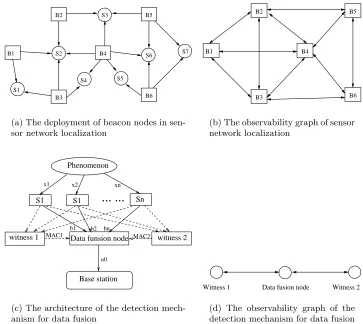
Example 1: Localization in sensor networks. The approach for detecting compromised beacon nodes [16] described in section 2.1 can be modeled by our framework as follows.
1. Observability graph. The vertices of the observability graph only includes beacon nodes. There is a bi-directional edge between two beacon nodes, if they are close enough to probe each other. (Note that a detecting beacon node has to use a pseudoID to prevent a compromised beacon node from recognizing a probing query) Figure 7(b) shows the observability graph corresponding to figure 7(a).
2. Alerts. If at timeta beacon nodeb1 detects a bogus location claimed by a nearby beaconb2,
it will send an alert (t, b1, b2) to the base station.
3. Sensor behavior model. The probability that an uncompromised beacon claims an incorrect location is determined by the resolution and the accuracy of the localization device. Let (x, y) be a beacon’s actual location and (x, y) be its measured location. Assumex−x andy−y
follow normal distribution N(0, σ2). Then the distribution of the distance d between (x, y) and (x, y) will be 2πd2σ2e−d
2/2σ2
. Suppose a beacon node is considered defected if dis larger than a pre-defined threshold. Then the reliability of beacon nodes isP(d < ).
Example 2: Sensor network data fusion. Data fusion is a common technique to reduce communication in sensor networks. Instead of having all the raw data sent to the base station, they are sent to nearby data fusion nodes, which aggregate them and forward the result further to the base station. Compromised data fusion nodes may send bogus aggregated information to the base station. Du et al. [5] proposed a witness-based mechanism to detect compromised data fusion nodes. The basic architecture of their approach is shown in figure 7(c). For a set of sensor nodes, there are one dedicated data fusion node and several witness nodes, all of which can receive raw data from sensor nodes. A witness node performs the same aggregation as the data fusion node, but only forwards the MAC of the result (using its shared key with the base station) to the data fusion node. The data fusion node then sends its result along with the witnesses’ MACs to the base station. The base station checks the consistency between the data fusion node’s result and the MACs of witnesses. Clearly, a compromised witness nodes may also send bogus MACs.
The above scheme can be modeled by our framework as follows.
1. Figure 7(d) shows the observability graph corresponding to figure 7(c). If there is a disagree-ment between the data fusion node and a witness, it is equivalent that they raise alerts against each other. In [5], sensor nodes collecting raw data are assumed to be trusted. Therefore, the observability graph only contains data fusion nodes and witnesses. The observability graph will be more complicated if we consider the situation where a node may serve as a witness or an aggregator for more than one set of sensors.
2. Alerts. If the MAC of a witnessw1 does not agree with the reported aggregation result of the
data fusion node df for an event happened at time t, the base station can derive two alerts
(t, w1, df) and (t, df, w1).
3. Sensor behavior model. We only need to derive the reliability rate for the data fusion node and witnesses. Suppose the communication channels between sensor nodes are reliable. Then the data fusion node and witness nodes will always receive the same data from the sensor node and get the same aggregation results. Thus the reliability rm of the data fusion node
and the witness nodes is 1.
4. Observer model. If we assume the communication channels between sensor nodes are reliable, then the data fusion node and the witness nodes will always send data to the base station when an event happens. Thus the observability rate rb = 1. The positive accuracy is the
probability that the MAC sent by an uncompromised witness does not agree with the bogus aggregation result from a compromised data fusion node, which equals to 1−2−k, where k
is the length of the MAC. The negative detection rate is the probability that the MAC from an uncompromised witness matches with the aggregation result from an uncompromised data fusion node, which equals torm.
B
Proofs
Lemma 3.1.
Proof. ⇒: Suppose there existsQi ⊆U ncompromisedCore(G, K), which satisfies|Qi|+
j=i|Bj| ≤
K. Then from definition 3.3,Qi∈Sgifor all 1≤i≤n, wherenis the number of valid assignments.
Suppose the corresponding set in the same coloring partition with Qi is Pi. Since Pi and Qi are
bipartite, we know that Pi ∈ Sbi for all 1 ≤ i ≤ n, thus Pi ⊆ CompromisedCore(G, K). Now
we look at a particular assignment (Sgx, Sbx), 1 ≤ x ≤ n, such that Sbx contains Qi and all Bj,
1≤j≤kexceptQi, wherekis the number of two-color partitions, andSgx containsPiand all Aj,
exceptQi. This assignment satisfies all constraints of definition 3.2, but it also introduces a
contra-diction: Qi ⊆U ncompromisedCore(G, K), thus Qi ⊆Sgj for all 1≤j ≤n, but Qi ⊆Sgx in this
assignment. So if we haveQi ⊆U ncompromisedCore(G, K), it must satisfy|Qi|+
j=i|Bj|> K. ⇐ : Suppose there exists someQi that satisfies |Qi|+
j=i|Bj|> K, andQi can be in some
Sby, 1 ≤y ≤n. Since each coloring partition will have a set in Sby, Sby will be composed of the
following sets: Sby = {Qi, Ar,· · ·, As, Bt,· · ·, Bm}. We thus have |Sby| > |Qi|+
since|Ai| ≥ |Bi|for 1≤i≤k. This contradicts with constraint 3 in Definition 3.2. So Qi must be
inSgy for all 1≤y≤n. ThusQi⊆U ncompromisedCore(G, K).
Corollary 3.1.
Proof. Suppose there exists some Bi ⊆ U ncompromisedCore(I, K), then we know Bi ∈ Sgi for
all assignment 1 ≤ i ≤ n. Thus Ai ∈ Sbi for all assignment 1 ≤ i ≤ n, so we have Ai ⊆
CompromisedCore(I, K). Now from Lemma 3.1, we have |Bi|+
j=i|Bj|> K. Since|Ai| ≥ |Bi|,
we also haveAi+
j=i|Bj|> K. Again from Lemma 3.1,Aimust be inU ncompromisedCore(I, K).
This introduces contradiction. SoBi⊆U ncompromisedCore(I, K).
Theorem 3.2.
Proof. The complexity of finding all the two-color partitions from the collusion inferred graph is
O(m), since we need to go through each edge to construct the partitions. The complexity of identifying the compromised core isO(n), since the number of the connected components is in the order ofO(n), and we need to go through each component. Thus the total complexity of algorithm
CollusionCompromisedCore isO(n+m).
Lemma 3.2.
Proof. When we assign the nodes into Sg, Sb, for each edge Eij, at least one end point of them is
inSb. So Sb is essentially a vertex cover forI. |S| ≥ |VI|.
Theorem 3.3.
Proof. ⇒: Suppose there exist somesthat satisfies|Ns|+CIs > K, ands∈Sgfor some assignment
(Sg, Sb). Then we will have Ns⊆Sb. According to Lemma 3.2, we know the minimum number of
malicious nodes inIs is CIs. So we have|Sb| ≥ |Ns|+CIs > K. This contradicts with constraint 3
of Definition 3.2. Sosmust be in Sb under any assignment. Thuss∈CompromisedCore(G, K). ⇐: If there exists s∈ CompromisedCore(G, K) that satisfies |Ns|+CIs ≤ K. Then we can
always construct an assignment ofSb: Sb =Ns
VIs. This assignment will satisfy all constraints
of Definition 3.2, but it also introduces a contradiction: s∈CompromisedCore(G, K), ands /∈Sb.
So if s∈CompromisedCore(G, K), it must satisfy |Ns|+CIs > K
Theorem 3.4.
Proof. From [18], the complexity of finding the maximum matching ofIs of any nodesisO(m√n).