Application of Deterministic and Stochastic Components of the Ocular Dynamic System.

ABSTRACT

WANG, XUEZHONG. Application of Deterministic and Stochastic Components of the Ocular Dynamic System. (Under the direction of Dr. Simon M. Hsiang and Dr. David B. Kaber.)

With the advent of eye tracking technology, gaze control is perceived to be an alternative way of human-machine interaction. Owing to the nature of eye movement, visually localizing a target is faster than by hand control and less likely to cause fatigue. Because of the connection between eye movement and attention, it is plausible to infer what targets may be of interest to people based on their gaze pattern. However, current design paradigms focus on fitting eye movements to user interfaces initially designed for hand movement. For example, many studies attempted to utilize gaze point as a mouse cursor, which resulted in limited success. To date, gaze-based interaction has been prone to mistakes and it is time consuming compared to other conventional non-keyboard input methods. Therefore, commercial eye tracking systems are almost exclusively used by people with severe disabilities or for military purposes.

previous models for hand movement are no longer appropriate for explaining dynamic features of the ocular plant.

By addressing these two differences between eye movement and hand movement, this dissertation aimed to improve the usability of eye tracking interaction and extend the existing goal-directed model for hand movement to three-dimensional eye movement. A prototype interface called the “Hot-Zone” was implemented for gaze-based interaction and assessment. Previous studies focused on utilizing gaze control for one-stage control such as „click‟ on an existing interface. The Hot-Zone acts like a context menu designed for gaze, which provides a solution to two-stage control, such as “Call out first, then select”. An experiment was conducted to show the performance of this technique compared with a conventional pointing device.

Because eye movement is closely related to information processing, it is possible to infer the task context (e.g., browse a picture on the web or read an article) by analyzing eye movement data. A system with predictive intelligence to evaluate a user‟s attention based on passive eye movement could be beneficial to support interaction quality and improve productivity. Hidden Markov Models and Support Vector Machine were used to differentiate reading and visual searching gaze patterns based on eye movement.

Application of Deterministic and Stochastic Components of the Ocular Dynamic System

by

Xuezhong Wang

A dissertation submitted to the Graduate Faculty of North Carolina State University

in partial fulfillment of the requirements for the Degree of

Doctor of Philosophy

Industrial and Systems Engineering Raleigh, North Carolina

2010

APPROVED BY:

________________________________ ______________________________

Dr. Simon Hsiang Dr. David Kaber

Co-chair of Advisory Committee Co-chair of Advisory Committee

DEDICATION

BIOGRAPHY

ACKNOWLEDGMENTS

I owe my deepest gratitude to Dr. Simon Hsiang, my advisor and Dr. David Kaber, my co-advisor, for their support and guidance. I am also heartily thankful to my committee

TABLE OF CONTENTS

LIST OF TABLES ... viii

LIST OF FIGURES ... ix

LIST OF SYMBOLS ... xii

1 Introduction ... 1

1.1 Motivation ... 1

1.2 Research scope and deliverable results ... 3

1.3 Organization ... 4

2 Literature review ... 5

2.1 Ocular anatomy and physiology ... 5

2.1.1 Globe and retina ... 5

2.1.2 Extraocular muscles (EOMs) ... 8

2.1.3 Eye movements ...11

2.1.4 Noise in eye movements ... 12

2.2 Gaze control for interaction ... 14

2.3 Gaze pattern recognition ... 17

2.4 Approaches for pattern recognition ... 19

2.4.1 Hidden Markov Models (HMMs) ... 19

2.4.2 Support Vector Machines (SVMs) ... 24

2.5 Eye rotation model in three dimensional space ... 30

2.5.1 Problem description ... 30

2.5.2 Eye movement in one dimension ... 30

2.5.3 Eye movement in three dimensions ... 33

2.5.4 Velocity-to-position integrator in three dimensions ... 38

2.5.5 Donders‟ Law, Listing‟s Law and half angle rule ... 40

2.6 Motor control strategies for goal-directed movements ... 41

2.6.1 The recursive approach ... 41

2.6.2 The optimal control approach ... 45

2.7 Summary ... 50

3 Pilot work ... 51

3.1 Apparatus ... 51

3.2 Application of voluntary eye movements – Hot-Zone ... 53

3.2.1 Objectives and hypotheses ... 53

3.2.2 Introduction ... 53

3.2.4 Results ... 56

3.2.5 Discussion ... 60

3.3 Gaze pattern recognition ... 61

3.3.1 Objectives and hypotheses ... 61

3.3.2 Methods... 61

3.3.3 Results ... 62

3.3.4 Discussion ... 68

3.4 Deterministic and stochastic components for ocular dynamics ... 68

3.4.1 Objectives and hypotheses ... 68

3.4.2 Deterministic component modeling ... 69

3.4.3 Stochastic component modeling ... 78

3.4.4 Methods... 82

3.4.5 Results ... 83

3.4.6 Discussion ... 87

4 Hot-Zone – a gaze interface ... 89

4.1 Research objective ... 89

4.2 Introduction ... 90

4.2.1 Hot-Zone overview ... 90

4.2.2 Local calibration ... 92

4.2.3 Hot-Zone component ... 94

4.3 Methods... 99

4.3.1 Task and equipment ... 99

4.3.2 Participants ... 101

4.3.3 Experimental design... 101

4.4 Results ... 103

4.5 Discussion ... 108

5 Differentiating reading and searching gaze patterns ... 111

5.1 Research objective ... 111

5.2 Feature selection ...112

5.3 Methods...115

5.4 Results ...115

5.5 Discussion ... 123

6 Modeling tradeoff between time-optimal and minimum energy in saccade main sequence ... 126

6.1 Research objective ... 126

6.2 Introduction ... 126

6.4 Results ... 132

6.5 Discussion ... 135

7 Conclusions and future research ... 140

7.1 Conclusions ... 140

7.2 Future research ... 141

LIST OF TABLES

Table 2-1 Specific research questions to be answered by this chapter ... 5

Table 2-2 Rotation directions and functions of extraocular muscles (EOMs) ... 9

Table 2-3 Classification of eye movements ... 12

Table 2-4 Levels of noise in the human body ... 13

Table 2-5 ISO 9241, CD Part 9: Non-Keyboard Input Devices requirement (applicable part) ... 17

Table 2-6 Summary of questions for literature review ... 50

Table 3-1 t-test for eye tracking and mouse, Test 1 ... 60

Table 3-2 t-test for eye tracking and mouse, Test 2 ... 60

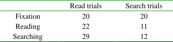
Table 3-3 Results of gaze pattern recognition ... 67

Table 3-4 Stochastic component of ocular dynamic models ... 79

Table 3-5 Experimental conditions (direction is not listed here) ... 83

Table 4-1 Manipulation schemes for manual and gaze control ... 92

Table 4-2. Experiment setup ... 102

Table 4-3 Experiment design ... 102

Table 4-4 Descriptive statistics ... 104

Table 4-5 Univariate analysis for completion time ... 106

Table 4-6 Variance structure estimates on completion time ... 106

Table 4-7 Univariate analysis for correct selection rate ... 106

Table 4-8 Variance structure estimates on correct selection rate ... 107

Table 5-1 Recognition rate statistics ... 122

LIST OF FIGURES

Figure 2-1 Sagittal section of adult human eye (Kolb, Fernandez & Nelson, 2008) ... 6

Figure 2-2 Structure of retina (Kolb, et al., 2008) ... 7

Figure 2-3 Distribution of cones in human retina, reproduced from (Curcio, Sloan, Packer, Hendrickson, & Kalina, 1987) ... 8

Figure 2-4 Rotation axes of eyeball ... 9

Figure 2-5 Extraocular muscles with motor nerves, anterior (Patrick et al.) ... 10

Figure 2-6 EyePoint test application with GUIDe: Point at the balloon... 15

Figure 2-7 Eye movement patterns for reading (left) and visual search (right) ... 18

Figure 2-8 Hidden Markov Models for pattern recognition ... 20

Figure 2-9 Left-right (left) and full connected (right) HMMs ... 22

Figure 2-10. Linearly separable data ... 26

Figure 2-11. Linearly overlapping data ... 28

Figure 2-12 The oculomotor integrator in one dimension ... 33

Figure 2-13 Non-commutative rotation in three-dimensional space ... 34

Figure 2-14 Head-fixed and eye-fixed frames ... 35

Figure 2-15 Two types of Gimbal sets reproduced from Haslanter (1995) ... 37

Figure 3-1 Components of pilot work ... 51

Figure 3-2 ASL EH 6000 eye tracker ... 52

Figure 3-3 Hot-Zone layout ... 54

Figure 3-4 Manipulation of Hot-Zone ... 55

Figure 3-5 Interface for Experiment 2. ... 56

Figure 3-6 Eye tracking and mouse completion time, Test 1 ... 58

Figure 3-7 Eye tracking and mouse completion time, Test 2 ... 58

Figure 3-8 Mouse trials completion times for all three subjects ... 59

Figure 3-9 Mean completion times for eye tracking and mouse trials ... 59

Figure 3-10 Interfaces for reading trial (left) and visual search trial (right) ... 62

Figure 3-11 Velocity profiles for reading (left) and visual search (right) ... 63

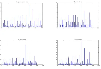
Figure 3-12 Scalar quantization ... 64

Figure 3-13 Short-time energy for reading and visual search ... 65

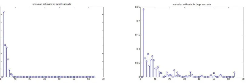
Figure 3-14 Initial emission matrix B0 estimation for small and large saccades ... 66

Figure 3-15 Parameter estimation convergence ... 67

Figure 3-16 Trained HMM for reading. S-small saccade, L-large saccade, F-fixation .. 67

Figure 3-17 Schematic diagram of the ocular dynamic model ... 69

Figure 3-19 Velocity function ... 72

Figure 3-20 The velocity function for a 7˚ saccade ... 73

Figure 3-21 Velocity function in oblique direction ... 74

Figure 3-22 Velocity profile of oblique saccade from experiment data ... 74

Figure 3-23 Vector rotation model in Simulink ... 77

Figure 3-24 Left: End point scatter plot; Right: fixational gaze points after saccades stop ... 78

Figure 3-25 Effect of target distance on endpoint variability (small target) ... 84

Figure 3-26 Effect of target size on endpoint variability ... 85

Figure 3-27 95% confidence ellipses of motor noise component prediction... 85

Figure 3-28 Endpoint scatter plot of experiment data ... 86

Figure 3-29 95% confidence ellipses on experiment data ... 86

Figure 3-30 Endpoint scatter and 95% confidence ellipses from (van Beers, 2007) ... 87

Figure 3-31 Accumulation error of simulation ... 89

Figure 4-1 Hot-Zone appearance ... 91

Figure 4-2 Offset (left) and local calibration (right) ... 93

Figure 4-3 Hot-Zone workflow. ... 94

Figure 4-4 Methods of the HotZoneLogicControl. ... 96

Figure 4-5 IEyeTracker interface. ... 97

Figure 4-6 ASLEyeTracker class. ... 98

Figure 4-7 The Hot-Zone with 6 peripheral zones. ... 99

Figure 4-8 Experiment task: Select the item. ... 100

Figure 4-9 Box plot of Completion time... 103

Figure 4-10 Box plot of Correct rate... 104

Figure 4-11 Correct selection rate vs. completion time percentile ... 107

Figure 5-1 Velocity profile ...113

Figure 5-2 Velocity for reading and visual search ...116

Figure 5-3 Duration histogram of reading and searching ...117

Figure 5-4 Saccades for read and search...118

Figure 5-5 Feature extraction (left: n=30, right: n=50) ...119

Figure 5-6 Recognition results with Support Vector Machine ... 120

Figure 5-7 Effect of batch size on recognition rate ... 121

Figure 5-8 Reading pattern with low recognition rate ... 123

Figure 6-1 Prediction error of duration. Left:θ = 25˚, Right: θ = 45˚ ... 133

Figure 6-2 Linear relationship between  and R ... 134

Figure 6-3 Weighting factor (/R) as a function of the amplitude  ... 134

Figure 6-5 Relation between qT (τ) and p2(t). ... 137

LIST OF SYMBOLS

J_{: Moment of inertia for the eye globe}

B_{: Viscous damping constant of the ocular system} K_{: Effective elasticity constant of the ocular system}

n

f

Natural frequency of the eye plant

 _{: Damping ratio of the eye plant}

m



: Peak velocity of saccadic eye movement

0



: Optimal saccade velocity constant, 450˚/s

0

A

: Optimal saccade amplitude constant, 7.9˚ A_{: Saccade amplitude}

1 2 3

{ ,h h h, }

: Head-fixed coordinate system

1 2 3

{ ,e e e, }

: Eye-fixed coordinate system υ_{: Axis of eye rotation}

( , )υ _{: Axis/angle representation of rotation} ( )

q t _{: Unit quaternion}

H_{: Set of quaternions} L_{: Listing‟s plane}

1

T

: Duration of the primary submovement

2

T

: Duration of the secondary (corrective) submovement

i

L

: Mean absolute distance to the center of the target after ith corrective movement

( )

S _{: Skew symmetric matrix operator}

R



: Saccade variance in radial direction 



: Saccade variance in tangential direction

( )t

 _{: Signal dependent noise}

( , , )

 A B π _{: Hidden Markov Model}

{ }a_ij



A

: State transition probability distribution matrix

{ ( )}b k_j



B

: Observable symbol probability distribution matrix { }i



π

1

Introduction

1.1 Motivation

The eyes are the windows to the soul. From a practical point of view, since the Stone Age, human history is very much defined by the evolution of hand tools. Nevertheless, the developments of eye tracking techniques for interaction remain in their infancy.

Existing eye tracking systems for human computer interaction are used almost exclusively for military purposes or by users with severe disabilities who do not have alternatives. Current design paradigms for gaze-based interaction treat the gaze end effector as a cursor to imitate manual control. Such practice violates the nature of eye movement, degrades the merits of eye tracking technology, and results in limited success. Such difficulties come from the fact that eye movement has unique characteristics different from hand movement. Equation Chapter (Next) Section 1

Due to the close relationship between visual perception and attention, passive eye movement is ubiquitous, which poses difficulties in determining a user‟s true intention. This ambiguousness is generally considered as a disadvantage of gaze interaction. As a result, eye movement dynamics are usually treated as noise and filtered out for practical purposes. Nevertheless, passive eye movement may be a rich source of knowledge to help identify gaze patterns such as reading and visual searching.

sinusoidal-shape velocity profile and impulse-step neural control signals (Meyer, Kornblum, Abrams, Wright, & Smith, 1988). However, hand movement is closed loop control with visual feedback. Most models developed to account for hand movement assume that the position of the end effector, either a fingertip or a stylus, is known during the movement. This assumption does not apply to eye movement, where the image on the retina is too blurry during the movement. The eye movement is more likely to be preprogrammed before the movement is initiated with no feedback correction during the course.

Eye movements comply with particular neural constraints. Donders‟ Law states that for each direction of gaze, the eyes assume the same position. Listing‟s Law indicates that when the eye moves to any position, it rotates about an axis that is perpendicular to the initial and final directions of gaze at the point of their intersection (Cannata & Maggiali, 2008; Martinez-Trujillo, 2005). The models for goal-directed hand movements can neither account for these features, nor explain the underlying control mechanism of eye movement.

realistic dynamic properties as inputs to a simulation model.

1.2 Research scope and deliverable results

1. An interface widget the “Hot-Zone” was developed to facilitate interaction through eye tracking. An experiment was conducted to compare the performance of gaze-based interaction with conventional mouse interaction for a simple selection task with the context menu. This new widget can be integrated with existing software such as Microsoft Office etc. to extend the scope of usability for eye tracking technology. 2. Passive eye movements were studied to extract information about visual task context.

Hidden Markov Models and Support Vector Machines were tested for gaze pattern recognition intended to discriminate reading and visual searching.

1.3 Organization

2

Literature review

The objective of this chapter was to provide background relevant to the model development in terms of eye movement variability and eye tracking based applications. In particular, the following topics are to be discussed (Table 2-1):

Table 2-1 Specific research questions to be answered by this chapter

Question Related background

What are the components of the ocular system? Anatomy/Physiology

What is the function of eye movement? Biomechanics

What are the challenges with existing eye tracking techniques for HCI applications?

Human factor How can unintentional eye movements be utilized? Pattern recognition What approaches are used for pattern recognition in this study? Pattern recognition How can the eye movements be represented in the three-dimensional

space?

Biomechanics What are the similarities and differences between eye movements and

hand movements?

Neurophysiologic What is the possible criterion that governs eye movement planning? Optimal control

Equation Chapter (Next) Section 1

2.1 Ocular anatomy and physiology

2.1.1

Globe and retina

film). The eye globe, as the camera body, is a slightly asymmetrical sphere with an approximate sagittal diameter of 24 or 25 mm and a transverse diameter of 24 mm.

Figure 2-1 Sagittal section of adult human eye (Kolb, Fernandez & Nelson, 2008)

The pupil is an aperture that allows light to enter (Figure 2-1). The dark color comes from the absorbing pigments in the retina. The iris is a circular muscle that controls the size of the pupil so that the amount of light allowed to enter the eye can be adjusted. The cornea is a transparent external surface covering both the pupil and the iris. This powerful lens produces a sharp image at the retina. The sclera is the supporting wall of the eyeball that is continuous with the cornea.

The lens, as the optical component, is a transparent body located behind the iris that is suspended by ligaments (zonular fibers), which are attached to the anterior portion of the ciliary body. Ciliary muscle actions contract or relax these ligaments and change the shape of the lens. This accommodation process is essential to focus an image of an object at distance on the retina (Kolb, et al., 2008).

same function as the film in a camera: to form the final image. Essentially, the retina is a piece of brain tissue that gets direct stimulation from outside light and images. The retina is a circular disc of approximately 22 mm in diameter. The center area of the retina is called the fovea, which is also the central point for image focus or the visual axis that provides the finest detail and directly transfers these detail to the brain for higher order visual perception. The central retina is a circular field of approximately 6 mm in diameter around the fovea while the remainder represents the peripheral retina stretching to the ora serrata (Kolb, 1991; Polyak, 1941; Van Buren, 1963).

The retina has a complex layered organization as shown in Figure 2-2. The innermost layer contains the ganglion cell axons that are the output neurons of the retinal, connected directly to the brain. The outermost layer consists of the pigment epithelium and choroid.

Figure 2-2 Structure of retina (Kolb, et al., 2008)

message and finally an electrical message that stimulates all neurons of the retina. There is a delicate difference between the retina and film, which could be an important factor in the proposed model for eye movement variability. That is, the film depends on the chemical reaction of the light-sensitive grains to record the pattern of light. Since the grains are sprayed evenly on the film, the developed image has a constant resolution. However, for the retina, anatomical evidence shows that the central retina close to the fovea is much thicker than the peripheral retina (Figure 2-3). The packing densities of photoreceptors, and the associated bipolar and ganglion cells increase in a radial direction toward the fovea. As a result, humans have the sharpest vision only at the central circular region that measures less than a quarter of a millimeter.

Figure 2-3 Distribution of cones in human retina, reproduced from (Curcio, Sloan, Packer, Hendrickson, & Kalina, 1987)

2.1.2

Extraocular muscles (EOMs)

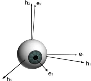
gimbal set. To describe the eye‟s orientation, it is necessary to define three orthogonal directions: horizontal, vertical and torsional (Figure 2-4). It is reasonable to approximate the eyeball as rotating around a fixed single point, where three axes intersect. To be specific, several terminologies are commonly used for describing eye rotation in three-dimensional space. Abduction is the horizontal rotation away from the nose, whose complement is adduction, the rotation toward the nose. Elevation and depression are the vertical rotations in opposite directions. Intorsion and extorsion are the rotations of the top of the cornea toward and away from the nose respectively (Table 2-2).

Figure 2-4 Rotation axes of eyeball

Table 2-2 Rotation directions and functions of extraocular muscles (EOMs)

Extraocular muscle Rotation direction Primary function

Medial rectus (a) Horizontal Adduction

Lateral rectus (b) Horizontal Abduction

Inferior rectus (c) Vertical Depression

Superior rectus (d) Vertical Elevation

Inferior oblique (e) Torsional Extorsion

Superior oblique (f) Torsional Intorsion

It should be noted that although there are three degrees of freedom, the eye does not assume all possible torsional rotations. Torsional movements are necessary to minimize the

Torsional

Horizontal

tilt to stabilize perception of horizontal lines, but they only become apparent when they are exaggerated by pathological processes. The eye rotations around the three axes are implemented by three pairs of complementary muscles attached to each eye: superior (Figure 2-5 d) and inferior (c) rectus muscles, medial (a) and lateral (b) rectus muscles, and superior (f) and inferior (e) oblique muscles.

Figure 2-5 Extraocular muscles with motor nerves, anterior (Patrick et al.)

The medial and lateral recti simply produce adduction and abduction, and the actions of the four remaining muscles are complicated because each of these muscles has some torsional component to its action. To reduce complexity, the model is limited under the condition that the inferior and superior recti produce depression and elevation only, and the superior and inferior obliques produce intorsion and extorsion. Experiments indicated that such an arrangement is a reasonable approximation, given that the saccade amplitude is within a certain range, e.g., 15 degrees (Raphan, 1998). It should be pointed out that although EOMs have the same functionality as a gimbal set, there are clear differences between the two regarding rotational kinematics, which will be covered in Section 2.1.4.

c

a

f

e

b

2.1.3

Eye movements

Globe, retina and extraocular muscles are the low-level building blocks for the ocular system. When people visually observe the surrounding environment, eye movement, plays an important role in connecting the external stimulus with the low-level components. Based on their functions and neurological differences, eye movements are generally classified into four categories: saccade, pursuit, vergence, and vestibule-ocular (VO) (Robinson, 1968).

Saccades are rapid eye movements with velocities as high as 800˚ per second. They occur frequently when we read or look at a scene, searching for an object. During saccades, sensitivity to visual input is reduced because the eyes are moving so quickly that only a blur image would be perceived on the retina. In other words, we don‟t receive information during saccades. The peak velocity and duration of the saccade is mostly determined as a function of the distance covered by the eye movements. Pursuit eye movements occur when the eyes follow a slowly moving target. Vergence is a conjugate movement which means the two eyes rotate in the opposite direction to accommodate the change of visual field depth. Vestibule eye movements occur to compensate head movement and keep a target on the fovea (Table 2-3).

Table 2-3 Classification of eye movements

Eye movement Directions Peak velocity Function Saccade Conjunctive 400- 800˚/s Switch focus

Pursuit Conjunctive Up to 100˚/s Follow slow motion target

Vergence Conjugate 20˚/s Make focus clear

VO Conjunctive 300˚/s Compensate head motion

Fixational Random 60 Hz Keep firing neuron spikes

There exist three types of small movements: nystagmus, drifts, and micro-saccades, which are also known as fixational eye movements. Due to these micro eye movements, the eye balls are never really still. Nystagmus is the constant tremor of the eyes, whose magnitude is quite small. Nystagmus is generally considered to be related to perceptual activity in that it keeps firing the nerve cells in the retina. Drifts and micro-saccades are often larger movements in magnitude than the nystagmus. Drift is a small and slow movement caused by the less than perfect control of the oculomotor system. Micro-saccades are small rapid movements to compensate for drift (Rayner, 1998). In this study, saccadic eye movements were carefully investigated. Saccades could be utilized for study of real world applications since they reflect visual attention processes. The motor control mechanisms that underlie saccades are also of general interest for both academic and practical purposes.

2.1.4

Noise in eye movements

the system that depend on the initial state and input for each movement. The second source is pure noise that can be characterized by certain probability density functions. In accordance with the information flow of external stimuli, three types of noise - sensory noise, cellular noise and motor noise - affect the system at three levels (Table 2-4).

Table 2-4 Levels of noise in the human body

Noise Source Example

Sensory noise Magnitude of the signal;

anatomy and physiology structure

Quality of the image, distance to the focus

Cellular noise Action potential (AP) variance of neuronal cell

Electrical noise & synaptic noise Motor noise Number of firing motoneurons

and muscle fibers

Signal dependent noise

Sensory noise is introduced during the perception stage when the external sensory stimulus is converted and amplified into a chemical signal. For visual perception, photons are absorbed by photoreceptors on the retina and converted to electrical signals. Consequently, the photoreceptor density, and its ability to accurately respond to a stimulus, sets a limit for perception. The second category is cellular noise that involves electrical noise and synaptic noise. Electrical noise is related to membrane potential fluctuations in the absence of synaptic inputs (van Rossum, O'Brien, & Smith, 2003). Synaptic noise refers to the trial-to-trial variability in the post-synaptic response (Kleppe & Robinson, 2006).

increase, accordingly (Henneman, 1957).

Because of these physiological properties of the motorneurons and muscle fibers, as well as the variance of action potential (AP) timing (Christakos, Papadimitriou, & Erimaki, 2006; Frank, Friedrich, & Beek, 2006), the variability in the generated force is proportional to the average force produced by that muscle (Jones, Hamilton, & Wolpert, 2002). Experimental and theoretical evidence revealed that the proportional variability of force is an inescapable consequence of the organization of the motoneuron and muscle fibers. Noise is an important factor in formulating the principles of the nervous system, which is the key to understanding the control mechanism and modeling realistic dynamic profiles of motor movement.

2.2 Gaze control for interaction

Eyes always fixate at a target before any hand movement is initiated. This indicates that eye tracking can be an alternative with superior potential for human-computer interaction (HCI) (Jacob, 1990). Past studies (Shumin, Carlos, & Steven, 1999) mostly focused on utilizing the gaze point as a mouse cursor to manipulate existing interface widgets. Those studies resulted in limited success attributable to distinct differences between eye and hand movements.

operate the system. In 1999, Zhai et al., developed a Manual And Gaze Input Cascaded (MAGIC) pointing system (Shumin, et al., 1999). By using this system, manual controlled pointing and selection were aided by eye tracking. Although the MAGIC pointing techniques were expected to provide potential advantages, such as reduction of manual stress and fatigue and shorter performance time for large magnitude pointing operations, the benefit gained by using eye-tracking technology was not promising.

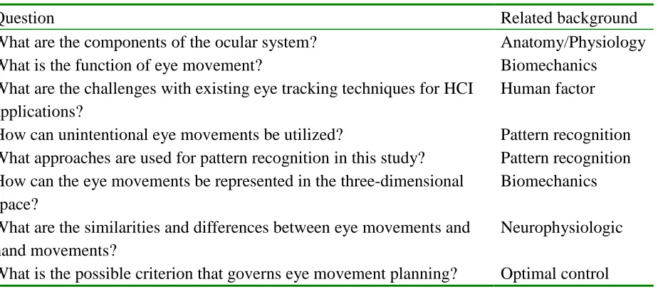
Recently, the HCI group at Stanford University developed a gaze-based interaction system {Kumar, 2007 #45} called Gaze-enhanced User Interface Design (GUIDe), which explored the effectiveness of utilizing gaze information as an augmented input besides the keyboard and mouse. The system provided a two-stage object selection sequence that presents a magnified “confident area” in the first stage as a basis for the user to adjust more precisely in the second stage. To fully cover the functions of a mouse, the system designated six hotkeys in the number pad for users to work with. To evaluate the usability of their system, several real world tasks, such as web browsing were tested (Figure 2-6). Qualitative results showed that 75% of the subjects preferred to use EyePoint instead of the mouse for faster and easier control. However, the error rate was much higher than the mouse input.

Table 2-5 ISO 9241, CD Part 9: Non-Keyboard Input Devices requirement (applicable part)

Requirement topic Mouse Eye tracking

Fine positioning anchor √

Repositioning possible without tools √ √

Feedback provided √ √

Resistance to unintended input √

Access from work position √ √

Visual feedback on input √

2.3 Gaze pattern recognition

Figure 2-7 Eye movement patterns for reading (left) and visual search (right)

Consider English reading tasks as an example. Eye fixations last about 200-250 ms and mean saccade amplitude is 7–9 letter space; most are made from left to right. Interestingly, it was found that word length has a direct impact on the probability of fixation. For example, 2-3 letter words are fixated about 25% of the time while words of 8 letters or longer are almost always fixated (Rayner & McConkie, 1976). Comparatively, visual search is much less stereotypical. Saccades are made more frequently with larger directional variance, and fixation duration is determined by the nature of currently fixated information (Vaughan, 1982). When searching for words, the word length no longer influences fixation duration (Rayner, Sereno, & Raney, 1996).

designing assistant devices to support user performance in tasks. In this study, Hidden Markov Models (HMMs) and Support Vector Machines (SVMs) were tested to identify reading and search behaviors from eye movement data. As the most popular approaches for pattern recognition, these two methods are briefly introduced in next section.

2.4 Approaches for pattern recognition

2.4.1

Hidden Markov Models (HMMs)

Hidden Markov Models were chosen for this application based on the following methodological requirements: (a) the model must be suitable for real-time implementation, (b) it must have a low computational cost; and (c) it must be robust to noise. Hidden Markov Models, as a statistical classification method, are capable of addressing all the three conditions. In fact, HMMs are an extensively applied tool, which dominant human behavior recognition applications such as speech recognition (both isolated word and continuous) and handwriting recognition (both on-line and off-line). Given a well-trained model, the computational cost is low. In addition, problems such as boundary detection, which commonly occur in other methods (i.e., dynamic time warping) are eliminated.

sequence. The two phases are interdependent in that the appropriate feature is closely related to the topology and recognition unit of the HMMs.

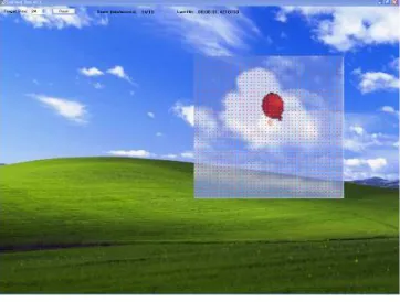
Raw Data: Voice signal, hand writing, eye movement etc Feature extraction Probability Calculation λA Probability Calculation λB Probability Calculation λC

HMM for A

HMM for B

HMM for C

Max λ

P(O|λA)

P(O|λB)

P(O|λC)

Figure 2-8 Hidden Markov Models for pattern recognition

Definitions and notations

To fully describe a HMM, a compact triple parameter notation is used: ( , , )A B π , Where A{ }a_ij is the state transition probability distribution matrix,

1

( | )

ij t j t i

a P q_ S q S { ( )}b k_j



B is the observable symbol probability distribution matrix,

( ) ( | )

j t k t j

b k P O V q S

{ }i



the model starting at statei. To be coherent, the probability matrix needs to satisfy: , ( ) 0, , ,

1 , ( ) 1 ,

ij j

ij j

j k

a b k i j k

a i

b k j

 

 

 





The HMM assumes the Markov assumption, which indicates that the state at time t1 only depends on the state at time t . In other words, it‟s assumed that the current state is conditionally independent of all previous states except for the most recent.

1 1 1 1

1 1 1 1

( _t t | _t t, _t t , , ) ( _t t | _t t) P q_ S  q S q_ S  q S P q_ S  q S

Since a HMM is a two stage process, it also assumes the Markov assumption for output symbol generation. Therefore, the probability of a particular symbol generated at time t

only depends on the state at that moment, and is independent of the past.

1 1

1 1

( _{t k}| _t t, _t t , , ) ( _{t k} | _t t) P O V q S q_ S  q S P O V q S

With the above two assumptions, conditional probability can be easily factorized by the Bayesian equation. Although these assumptions limit the memory of the HMM, they reduce the number of parameters to be determined, and they make it possible for learning and decoding algorithms to be extremely efficient.

HMM topology

used for both the state transition matrix and the output matrix. To apply probability calculations, each frame of the extracted feature must be represented by a symbol from a finite alphabet. Vector quantization is usually used during this data compression procedure.

S1 S2 S3

S1 S2

S3

Figure 2-9 Left-right (left) and full connected (right) HMMs

There are also continuous HMMs that use continuous density functions, most commonly multivariate Gaussian density, in which an output probability density function is described by a mean vector and a covariance matrix. This approach provides a distribution that is more accurate and can directly estimate the parameters. However, such advantages are achieved at the cost of a considerably higher computational load. As a result, they are generally inefficient, and inconsistent in performance.

Many researchers have conducted experiments comparing discrete and continuous HMMs. Studies in speech recognition suggest that discrete HMMs perform better because of their efficiency in calculation and capability to represent any distribution. Given the nature of this application, discrete HMMs were used for gaze pattern recognition.

Solutions to the three fundamental problems in HMMs

problems deal with training the HMMs, and solutions are aimed at determining the parameters in the triple notation to maximize the probability of the observation sequence given the model. This learning problem is usually difficult in terms of obtaining a global optimal solution. The Baum-Welch method (also known as the expectation maximization method) provides a locally optimized solution with an interactive procedure.





t 1 2

T t 1 t+1

1

1

1 t+1 1 t+1

1 t+1

Let ( ) ( , | )

( ) 1 ( ) ( ) ( )

Let ( ) ( | , )

( , ) , ,

( ) ( ) ( ) ( ) ( ) ( )

( , )

( | ) ( ) ( ) ( )

t t T t i

N

ij j t i

t t i

t t i t j

t ij j t t ij j t

t

t ij j t

i P O O O q S

i j a b O j

i P q S O

i j P q S q S O

i a b O j i a b O j

i j

P O i a b O j

                                   







1 1 ( , ) T t t i j   



expected number of transitions from state S_i to S_j Formally, the Baum-Welch algorithm can be defined as follows:

(i) assume an initial HMM ₀ (A B π₀, ₀, ₀)

(ii)re-estimate the parameter matrices with the following equations:

1 1

1, 1

1 1 1

1 1 ( ) ( , ) ( ), , ( ) ( ) ( ) t k T T t t

t O V t

i ij T j T

t t

t t

i i j

i a b k

i i                 









(iii) Check convergence criteria; if satisfied, exit the loop, otherwise, go to step (ii) To evaluate HMMs, P O( | ) must be calculated, given the observation sequence

1 2 T

complexity from 2TNT to 2

N T. The induction can be formulated as follows









t 1 2

1 1 t+1 t 1

1

T 1

Let ( ) ,

( ) ( ) ( ) ( ) ( )

( )

t t i

N

i i ij j t

i N

i

i P O O O q S

i b O j i a b O

P O i

                _{  }   





where_t( )i is the probability of the partial observation sequence { ,O₁ O_t} (1 t T) with the hidden state i at time t given the model. To determine the most probable internal state sequence, a dynamic programming method called the Viterbi algorithm is employed. Since this method is not used in the present study, it is not discussed here. More detailed information can be found in other papers or books on the HMM topic (Rabiner, 1989).

2.4.2

Support Vector Machines (SVMs)

Introduction

provides background on applying SVMs to learn from sampling data and solve pattern recognition problems. Consider a binary classification problem with n training samples, given as: ( ,x₁ y₁), (x₂,y₂), , (x_n,y_n), x_i l, y









( , , ) T

f x w b w xb, which labels training samples.

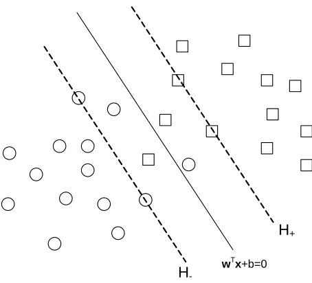
Linear maximal margin classifier for linearly separable data

When the training data set is linearly separable, the hyperplanes obtained perfectly separate training samples into two classes:









sign , ,

1 0

,

1 0

i i

T i T

i

y f b

b b



  

 _{  } 

x w w x w x

(2-4)

wTx+b=0

H+

H

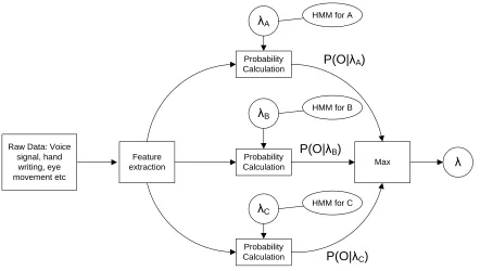
-Figure 2-10. Linearly separable data

A canonical hyperplane satisfies w xT _i b 1 and SVMs search for the optimal canonical hyperplane, which have a maximal margin. Specifically, we denote

: T 1

H_ w x b and H_:w xT   b 1 as training samples in the canonical hyperplanes, which are support vectors. Consequently, the margin M  2

w , which indicates that to find the hyperplane with a maximal margin is equal to minimizing w . This approach can be formulated as a convex quadratic programming problem:

1 2 ( , )

min

. . ( ) 1

1, 2, ,

T b

T

i i

s t y b

i n

  

w w w

w x (2-5)

This optimization problem is solved by the saddle point of the Lagrange function:

1 2

1

( , , ) ( ) 1

n

T T

i i i

i

L b  y b



 

 



The Karush-Kuhn-Tucker (KKT) conditions for this function to be optimum are as follows: * 1 1 0, 0, 0 n

i i i i n i i i L or y L or y b          _{ } 





The following complementary conditions must also be satisfied:





1 0 0, 1, 2, ,

T i i T i i y b y b i n                 w x

w x (2-7)

Substituting (2-6) into L( , , )w b α , the primal problem is formulated as:

1 2

min

. . 0,

0 T T T s t   

α Hα f α y α

α

Where H denotes the Hessian matrix of this problem H_{i j}  y y_{i j}(x xT_{i j}) and f is a unit vector f 





Linear soft margin classifier for overlapping classes

wTx+b=0

H+

H

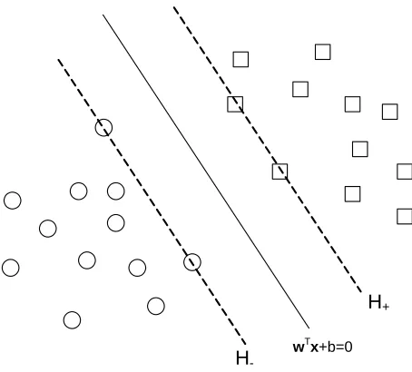
-Figure 2-11. Linearly overlapping data

The width of a soft margin is controlled by a penalty parameter C chosen by the user. The constraints are relaxed by introducing slack variables _i , i1, ,n. Constraints are rewritten as y_iwTxb_ 1 _i . The problem is reformulated with the penalty parameter C:

1 2 ( , , )min

. . ( ) 1

0, 1, 2, ,

T b

T

i i i

i

s t y b

i n

 

  

 

w ξ w w

w x (2-8)

The Lagrange function is:

1 2

1 1 1

( , , , ) ( ) 1

n n n

T T

i i i i i i i

i i i

L b C   y b   

  

 

 

 



w α β w w w x





1 0, 1, ,

n

i i i i n i i i i i T

i i i i

L or y L or y b L or C

y b i n

         _{ }                  





The resulting dual problem is very similar to the separable cases:

1 2

min

. . 0,

0 , 1, ,

T T

T

i

s t

C i n



 

  

α Hα f α

y α (2-10)

The final quadratic optimization problem is the same as the separable case, the only difference is that an upper bound C is now applied to each _i.

Nonlinear classifier

The SVM method can be extended to handle nonlinear classification problems by transforming training samples to a higher dimensional space with a mapping :

l m

  _.

Linear SVMs are then applied to separate the classes in the feature space m. The dual problem is then formulated as:

1 2

min

. . 0,

0 , 1, ,

T T

T

i

s t

C i n



 

  

α HKα f α

y α (2-11)

1

sign ( , )

n

j i i i j

i

y  y K x x b



 

 _  _





2.5 Eye rotation model in three dimensional space

2.5.1

Problem description

Eye movement is the direct outcome of extraocular muscle contractions. The forces applied by the EOMs determine the dynamic features of the eye movement such as trajectory and velocity profile. The transition from the force to the final gaze orientation is rather mechanical and complies with the same physical principles as any other rigid body rotation. Information presented in this section is important for modeling the deterministic component of the ocular dynamic system, where the neuronal constraints that specifically apply to the eye movement are also introduced. These rules, along with the physical principles will be developed rigorously in Chapter 3.

2.5.2

Eye movement in one dimension

The analysis of eye movement is relatively standardized, and with less degree of freedom compared to the analysis of limb movement. The relationship between dynamic components, such as amplitude, duration and peak velocity, has been well established by regression and exponential models, as in the following equations (Collewijn, Erkelens, & Steinman, 1988).

0

0 (1 )

A A

m e

    (2-12)

2.7 23

where _mis the peak velocity (degrees per second), and d is the duration in milliseconds. This relationship is also called the “main sequence” of saccadic eye movement. Both _m and d are determined almost exclusively by the amplitude A. ₀ and A₀ are the constant coefficients determined by the experiment. Although these equations were established for horizontal saccadic eye movements, they are also fair approximations for saccades in oblique directions. Since eye movement, like any other mechanical movement, involves the physical qualities of force and mass, it can be modeled as a differential equation relating displacement to force or torque applied. The first eye movement model (2-14) made connections between eye position  and the firing rate of ocular motoneurons, which innervate extraocular muscles and generate force (Westheimer, 1954; Young & Stark, 1963). These early models were later confirmed by directly recording the firing rate R of the motoneuron and refined as follows:

Rmrk (2-14)

The coefficients k, r and m are the slopes of the linear regression fit to the experimental data (Robinson, 1970; Skavensk.Aa & Robinson, 1973). Although the scale of the three slopes changes with the amplitude, Robinson found that the ratio between them was relatively constant. The existence of such a relationship was observed by neurological experiments (Robinson, 1970). Given that changes in the discharging rate of the motoneuron causes changes in muscle force, Equation (2-14) can be rewritten as

TJBK (2-15)

compatible with the neurological structure and can be modified to agree with experimental eye movement data by adjusting the ratio of the three parameters (Robinson, Gordon, & Gordon, 1986). For theoretical studies, a second order differential equation has been widely accepted for one-dimensional saccadic eye movement:

1 2

1 2 1 2

1 2

1 2

1 2 1 2

1 2

1 2 1 2

1

1

1, , ,

1 1

,

2 2 2 2

n

t t T

t t t t

t t B

J B K t t

t t t t K

t t

K B

f

J t t KJ t t

                     (2-16)

where f_n is the natural frequency, and  is the damping ratio. fn and  are

eye movements (Leigh & Zee, 1999). This velocity-to-position integrator plays a central role in understanding how the ocular motor system produces kinematically efficient behavior since this transforming process occurs during all kinds of eye movements.

Figure 2-12 The oculomotor integrator in one dimension

2.5.3

Eye movement in three dimensions

brief review of these mathematical tools will be covered and one of them will be chosen for the modeling work.

Figure 2-13 Non-commutative rotation in three-dimensional space

Figure 2-14 Head-fixed and eye-fixed frames

The orientation of the eye-fixed coordinate system in regards to the head-fixed coordinate system could then be described with a rotation matrix R of the form

1 1 2 1 3 1

1 2 2 2 3 2

1 3 2 3 3 3

i i

e Rh

e h e h e h R e h e h e h e h e h e h



  

 

 

_    _

    

 

(2-17)

R belongs to the special orthogonal group of order three (SO(3)), which holds the following properties:

(a) RT R1SO(3)

(b) Columns (therefore the rows) of R are mutually orthogonal (c) Each column (therefore each row) of R is a unit vector (d) det( ) 1R 

conventional methods to parameterize an arbitrary rotation: the Euler-angle representation, the roll-pitch-yaw representation, and the axis/angle representation.

The Euler-angle representation is extensively used in classical mechanics of rigid bodies and many other applications. The eye orientation in regards to the head can be specified by three angles( , , )   , which are referred to as Euler angles. The sequence of the rotational composition is critical to obtain the correct result. For example, we first rotate about h2 by the angle . Next, rotate about the e1 axis by the angle  and finally rotate

about the e₃ axis by the angle  . The rotational transformation can be described as the composition of three rotation matrices

2, 1, 3,

h e e

RR R R  (2-18)

It should be noted that there is no uniform standard regulating the order of the axes when applying a sequence of rotations. As a result, there are twelve possible conventions regarding the Euler angles in use and proper definitions should always be stated before employing Euler angles (Spong, et al., 2006).

Figure 2-15 Two types of Gimbal sets reproduced from Haslanter (1995)

This sequential style rotation conflicts with the physiological properties of eye movement that the three pairs of extraocular muscles apply their torques simultaneously on three nearly fixed axes. Therefore, the composition of the three components of rotation is mutually interdependent. Such an anatomical arrangement favors a symmetric representation of eye orientation, which will be introduced in the following sections.

According to Euler‟s theorem, an arbitrary eye position can be achieved from the primary position by a single rotation about a fixed axis. Thus, the angle/axis representation is more efficient since it eliminates the ambiguity of the rotation sequences. Let

1 2 3

[ ,  , ]T



rotation vector model.

2.5.4

Velocity-to-position integrator in three dimensions

Quaternion model

To develop a three-dimensional analog of the velocity-to-position integrator, a quaternion was introduced as the substitute for the scalar counterpart in the one-dimensional model (Tweed & Vilis, 1987; Westheimer, 1957). Quaternion is a four-component representation of angular position discovered by Hamilton in the mid-19th century. Detailed instruction on and discussion of quaternion and their mathematical properties is beyond the scope of this paper. Here essential background material on quaternion is covered, which is used in the proposed model. Let Hdenote the set of quaternion. A quaternion q that uniquely specifies a rotation represented by ( , )υ is defined as

0 1 2 3 0

2 2 2

q ( q q q ) q ,

1, ,

q i j k q

i j k ijk ij k ji k

      

       

qI H

(2-19)

0

q is referred to as the scalar component and qrepresents the vector component. In general, a unit quaternion with length of 1 describes a pure rotation transformation

0

2 2 2

1 2 3

2 2 2 2

0 1 2 3

q cos 2

q q +q sin 2 q +q q +q 1

        q (2-20)

The derivative of a quaternion is given by 1 2 (0, ) q q



ω

ω ω

The vector part ωis the angular velocity of the eye in the head-fixed frame. With the position and velocity components represented by quaternion, Tweed et al. proposed a quaternion integrator (Tweed & Vilis, 1987) to replace the one-dimensional model in Equation (2-15). As for the relationship between the quaternion and rotation matrix, a detailed treatment can be found in other papers (Haslwanter, 1995). The general conclusion is that the two tools are equivalent since they are used to represent the same principles.

Vector model

For a unit quaternion, the scalar component is not independent and provides no additional information once the vector component is given. Thus, a rotation vector r

corresponding to a quaternion is given by:

0

tan 2 q



 q  υ

r (2-22)

Based on this relationship, another approach to model the oculomotor control utilizes rotation vectors (Raphan, 1998; Schnabolk & Raphan, 1994a). The main argument for this effort is that the quaternion model treats the orientation of the eye as the output of the integrator while neglecting the fact that the central nervous system (CNS) activates the muscles to generate the torque to rotate the eyeball.

Following this rationale, Raphan et al. proposed a vector integrator model that converts neural signals, representing an angular velocity, to a state variable xp. This state variable is

p p p p

n p p

n       

x H x G m C x D

m Mm r r (2-23) 1 1 (  )      

ω J Bω K υ J m (2-24)

  ω υ (2-25)





1 1

( ) ( ) cot

2 2 2



     

υ ω υ υ ω υ (2-26)

p

H is the system matrix whose eigenvalues determine the time constants of the integrator. G_p and C_p are the coupling matrices applied to input and output neural input. Dis the direct premotor-to-motoneuron coupling matrix. This model has the advantage that it resembles the neural and physiological aspects of eye movements (Raphan, 1998). However, the input to the model is the neural signal which is not easily available. Furthermore, it requires as many as eight parameters, most of which were approximated to be consistent with the dominant time constants associated with Equation (2-14). To justify the model and verify the parameters, a simulation was conducted with an assumed input signal and parameters from the work of Schnabolk and Raphan (1994b).

2.5.5

Donders’ Law, Listing’s Law and half angle rule

exists a specific eye orientation, called the “primary position”, from which other physiological orientations can be reached by a single rotation about an axis. During eye movements, the eyeball assumes a unique torsion for each possible eye orientation (Crawford, Martinez-Trujillo, & Klier, 2003). Listing‟s Law can be used as a touchstone to test the ocular dynamic model. This neural constraint also indicates that only sequential independent rotation representation should be considered in describing eye movement. One important implication of Listing‟s Law is the half angle rule, which states that though the eye rotation itself has no torsional component, the angular velocity axes should tilt out of Listing‟s plane by half the angle of the gaze‟s deviation from the primary position. Detailed explanation for Listing‟s Law and the half angle rule will be presented later in the Chapter.

2.6 Motor control strategies for goal-directed movements

2.6.1

The recursive approach

There are resemblances between limb movements and saccadic eye movements. From a physiological perspective, any body movements can be viewed as results of contracting opposing groups of agonist and antagonist muscles. For limb movement, Fitts‟ Law indicates that motion time is a function of target size and target distance. For eye movement, a similar linear relationship (also known as the main sequence) has also been observed, as mentioned in 2.5.2. Several goal-directed models were developed to explain Fitts‟ Law for limb movement, which cast insight on eye movement. In this section, we review and point out the limitations of these models before we introduce more sophisticated optimal control models.

The two-component model suggests that aiming limb movements consist of an initial impulse phase and a current control phase. The initial impulse phase is rapid and stereotyped and the second phase consists of slow motion adjustments guided by visual feedback. Woodworth examined the contribution of vision to the control loop and suggested that the time lag needed for visual feedback to be effective was approximately 450 ms.

In the 1950s, Fitts (Fitts, 1954) quantified a linear relationship, which governs hand movement as follows:

2

log (2 / )

MT  A B D W (2-27)

MT is the mean time to complete the movement. D is the distance from the start point to the center of the target. W is the width of the target along the axis of motion.

Following Woodworth‟s work (1899), several processing-based models were developed on the two-component model. In 1968, Keele and Posner substantially reduced the time lag estimate to 190~260 ms in an influential study, which addressed a flaw in Woodworth‟s experiments (Keele & Posner, 1968). These results provide physiological evidence that eye movement is an open-loop control process because most saccades last less than 200 milliseconds, which is not sufficient for visual feedback to be effective.

Other notable examples include the iterative correction model (Crossman & Goodeve, 1983), single-correction model (Beggs & Howarth, 1970, 1972) and the impulse variability model (Meyer, et al., 1988; Meyer, et al., 1982). All these models attempted to derive a form similar to Fitts‟ Law based on assumptions. For instance, the iterative correction model (Crossman & Goodeve, 1983) makes three assumptions:

1. There is a minimum time t for an initial movement and each corrective movement.

movements is constant.

3. The initial movement takes less time (expressed by a constant a) than the corrective movements.

Let L_i denote the mean absolute distance from the center of the target after the th

i corrective movement. With the preceding three assumptions, we can obtain the following





0 1

2 2

, / 2, /

/ 2 solve for :

/ (2 )

log log (2 / )

n i i

n n

n

L D L W L L K

L K D W

n

K W D

n K D W

          (2-28)

Then the mean completion time for the movement can be formulated as

2

2

( 1) ( 1) log (2 / )

/ log

MT n t t nt a a b D W

b t K

        

  (2-29)

Based on the iterative correction model and the impulse variability model, Meyer et al. (1982) developed the “optimized dual-submovement model”. The key idea is that the motor intelligence controls the movement subject to minimizes (or maximizes) certain performance criterion. For example, in manual positioning tasks, subjects are instructed to choose a control solution to minimize total movement time. This minimizes the average time to reach the target. This model predicts that average total movement time can be approximated by the equation:

1

1 1 2

2

n _n

i i

D

MT T T k k

W      _{   }  



T is the duration of the primary submovement. T ₂ is the duration of the secondary (corrective) submovement. n is the maximum number of submovements.