Quantum transport and dynamics of phonons in
mesoscopic systems
Thesis by
Deborah H. Santamore
In Partial Fulfillment of the Requirements for the Degree of
Doctor of Philosophy
1 8 9 1
C A L
IF
O
RN
IA
IN
ST I T
U TE O
F T E
C H
N
O
L
O
G Y
California Institute of Technology Pasadena, California
2003
c
° 2003
Acknowledgements
Firstly, I would like to thank Mike Cross for giving me the opportunity to work on challenging and interesting research projects. In spite of my many shortcomings, through his guidance, I have successfully picked up some of his research style over the years, which I hope to treasure and safeguard for life. His approach to physics is thorough and his comments always to the core of the problem. He has been truly my research father and he is and will be always the one I look up to.
Looking back on the second part of my PhD work it was rather a challenging project as well as fascinating. I have put one foot in condensed matter physics whilst the other foot in atomic physics/quantum optics, and tried to pull out the best of both fields at the interface. I have also made (sometimes effective and many other times futile) attempts to bridge the gap between the two fields with frequent help from astrophysics for order of approximations and numerical tricks. In course of my PhD research, I have been fortunate to benefit from interactions with several physicists in different branches, who are the leading figures in their respective fields. All of them took an interest in one as small as myself, have taken time from their busy schedule, and kindly helped and guided me. They even agreed to be on my PhD defence committee. Without their help and encouragement, I could not have survived.
I am grateful to Gerard Milburn for allowing me to visit and work with him at the SRC for Quantum Computer Technology at the University of Queensland. During the long stay, I have learnt from him numerous theoretical techniques used in quantum optics and atomic physics.
listening to a request from a student such as myself. His deep insights in physics have fascinated me from the very first meeting and his physics mind seems to be always filled with ideas. I also thank him for hosting me during my visit. His warm hospitality was superb and nobody could ask for more.
Kip Thorne had supported me on my formative year as a theoretical physicist. He is also famous for caring others and this legend has never failed me. I am grateful for his support and allowing me to attend his group meeting whenever I want to over the years.
I owe thanks to Michael Roukes for financial support in my final year. I also thank him for providing the information about exciting recent experimental developments in his group as well as addressing his great experimental insights.
It was fortunate that I have had an opportunity to interact with Andrew Do-herty. He introduced me to a world of quantum dynamics and measurement theory which have eventually brought forth a fruitful collaboration. He has been also very patient listening to my endless moans about the huge gap between quantum optics and condensed matter physics.
My Caltech life started with an interaction with Yuri Levin who had trained me in my infant years as a theoretical physicist until I was weaned. He was very much in favour of Newtonian mechanics and it showed from time to time: I had to unlearn Lagrangian mechanics in order to learn another, but I knew, at the end, his was correct and simpler. I also have enjoyed our collaboration very much.
It was a pleasure to meet Miles Blencowe. He has helped my earlier work by carefully reading manuscripts of my papers and providing useful suggestions as well as inviting me to visit him.
I sincerely express my thanks to Alexei Alexeevich Abrikosov for his kind reply to my e-mail a long time ago, which initiated my quest as a theoretical physicist. I also thank him for sharing some interesting stories about Lev Davidovich Landau.
if outsiders ever have had listened to our conversations, they would have wrongly thought we were fighting.
My heartfelt thanks go to Jonathan Tannenhauser, Ruben Krasnopolsky, and Dustin Laurence for their support, especially in the last few months of my thesis writing. I could not have completed my thesis without their help in proofreading, English grammar, and LaTeX typesetting.
Abstract
Recent advances in nanotechnology have shrunk the size of mesoscopic structures. This allows us to investigate the quantum mechanics of mechanical oscillators. In this thesis we focus on two aspects.
In Part I, an individual discrete mode structure of an oscillator and its effect to thermal conductance have been thoroughly examined: Specifically, we investigated the reduction in the thermal conductance in the quantum limit due to phonon scat-tering by surface roughness, first using scalar waves, then using full three dimensional elasticity theory for an elastic beam with a rectangular cross section. At low fre-quencies, we find power laws for the scattering coefficients that are strongly mode dependent, and different from the results deriving from Rayleigh scattering of scalar waves, that is often assumed. The scattering gives temperature dependent contribu-tions to the reduction in thermal conductance with the same power laws. At higher frequencies, the scattering coefficient becomes large at the onset frequency of each mode due to the flat dispersion. We use our results to attempt a quantitative un-derstanding of the suppression of the thermal conductance from the universal value observed in experiment.
Contents
Acknowledgements iii
Abstract vi
I
Quantum transport of phonons in disordered systems
1
1 Introduction and preliminary calculations 2
1.1 Ideal thermal conductance . . . 5
1.1.1 Analytical method using density of states . . . 5
1.2 Approximation methods to obtain cutoff frequencies . . . 6
1.2.1 Thin plate elastic theory method . . . 7
1.2.2 Bulk mode method . . . 8
1.2.3 Comparison of the different methods . . . 9
2 Surface scattering of phonons - the scalar model 11 2.1 Scattering formalism . . . 12
2.1.1 The model . . . 12
2.1.2 Green function method . . . 13
2.1.2.1 Scattering amplitude and Green function . . . 13
2.1.2.2 Green function . . . 13
2.1.3 Boundary perturbation . . . 15
2.1.4 Scattered field . . . 17
2.1.5 Roughness characterisation . . . 17
2.2 Comparison with the experiment of Schwab et al. . . 22
3 Detailed analysis of surface scattering effects - the elastic model 27 3.1 From a scalar model to an elastic model . . . 27
3.2 General formalism . . . 29
3.2.1 The model . . . 29
3.2.2 Incident and scattered fields . . . 33
3.2.3 Green function . . . 36
3.2.4 Boundary perturbation . . . 38
3.2.5 Scattering coefficient . . . 39
3.3 Thin plate limit . . . 45
3.3.1 Attenuation coefficient in the thin plate limit . . . 47
3.3.2 Evaluating the group velocity . . . 50
3.3.2.1 In-plane modes . . . 51
3.3.2.2 Flexural modes . . . 51
3.4 Scattering analysis . . . 58
3.4.1 Dispersion relation and group velocity . . . 59
3.4.2 Scattering behaviour . . . 60
3.4.3 Change in the thermal conductance . . . 65
3.5 Comparison with the experiment of Schwab et al. . . 66
3.5.1 Experimental geometry . . . 66
3.5.2 Roughness correlation function . . . 68
3.5.3 Individual mode contribution to the thermal conductance . . . 72
6 Deterministic dynamics - the master equation 82
6.1 Constructing the Hamiltonian . . . 82
6.1.1 The model . . . 82
6.1.2 System Hamiltonian . . . 83
6.2 Dynamics of the system: Master equation and adiabatic elimination 90 6.2.1 Master equation . . . 90
6.2.1.1 Thermal coupling component of the master equation (Lindblad form) . . . 90
6.2.2 Adiabatic elimination . . . 99
6.2.2.1 Evaluation of ˙ρP1 . . . 103
6.2.2.2 Evaluation of ˙ρP2 =−iλ 01 h a†0a0a†1a1, ρ i . . . 104
6.2.2.3 Evaluation of ˙ρP3 =−iλ 01 h a†0a0 ³ αa†1+α∗a 1 ´ , ρi . . 105
6.2.2.4 Adiabatically eliminating the ancilla operators . . . . 108
6.3 Analysis of the master equation . . . 110
7 Measurement statistics and stochastic dynamics - the stochastic master equation 115 7.1 Measurements and trajectories overview . . . 115
7.2 The measurement bath operator description of the current . . . 116
7.3 Quantum trajectories . . . 120
7.3.1 Background on quantum trajectories . . . 120
7.3.2 Quantum trajectory description of the measurement . . . 122
7.3.2.1 Unravelling a master equation . . . 122
7.3.2.2 Measurement current with a stochastic component . 123 7.3.3 Adiabatic elimination of the stochastic master equation . . . . 128
7.3.4 Accumulated projective measurements and thermalisation . . 135
7.3.4.1 The component with dt of Eq. (7.73) . . . 135
7.3.4.2 Dwell time between transitions . . . 136
7.3.4.4 Collapse time, measurement time, and ease of
observ-ing transitions . . . 138
7.3.4.5 The measurement time versus the dwell time . . . . 141
7.3.4.6 Effect of temperature . . . 143
7.4 Trajectories and experimental outcomes . . . 148
7.4.1 The stochastic master equation and the measured signal . . . 148
7.4.1.1 Stochastic master equation with an imaginary observer 151 7.4.2 Parameters and constraints . . . 152
7.4.2.1 Anharmonic coupling coefficient . . . 152
7.4.2.2 Damping rates and k/ν ratio . . . 153
7.4.2.3 Driving strength . . . 154
8 Anharmonicity - the effect of the nonlinear term 156 8.1 The Hamiltonian and master equation . . . 156
8.2 A damped driven anharmonic oscillator . . . 161
8.2.1 One-time correlations . . . 161
8.2.2 Two-time correlations . . . 165
8.2.3 Operator correspondences toc-numbers . . . 168
8.3 The master equation for the reduced density matrix . . . 171
8.3.1 Effects of the anharmonic terms . . . 172
8.3.2 Parameter constraints imposed by the anharmonic terms . . . 173
9 Conclusion to Part II 177 9.1 Future issues . . . 178
A Appendices to Part I 180 A.1 Optical theorem and S-matrix . . . 180
A.2 The second term of the total field equation . . . 181
A.3 Group velocity and energy velocity . . . 184
B.2 Wiener process . . . 189 B.3 Unravelling of a master equation for a heterodyne detection . . . 191 B.3.1 Derivation . . . 192
List of Figures
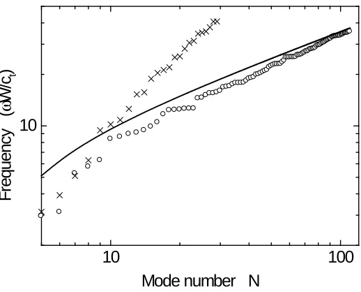
1.1 Mode cutoff frequency ωN as a function of mode number N. crosses: thin plate theory; circles: xyz algorithm; solid line: density of states calculation. A thickness to width ratio d/W = 0.38 was used. Bulk mode calculation is not shown here. . . 10
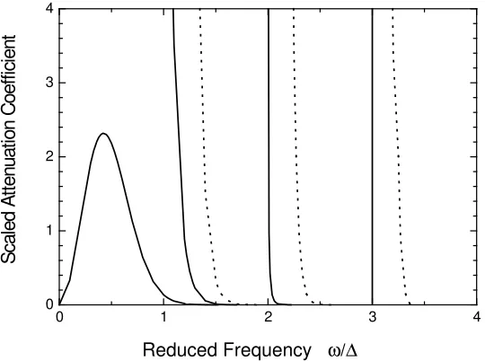
2.1 2-D model used for calculation of the scattering of elastic waves by rough surfaces. . . 12 2.2 Scaled attenuation coefficients (W4/δ2aL)|σ
−n,m|2 as a function of
re-duced frequency,ω/∆ where ∆ =πc/W withcthe velocity of the waves: solid—from mode m= 0 to mode −n,n = 0. . .3 and dashed—modem
to mode −m, m = 1. . .3. A value of the roughness correlation length
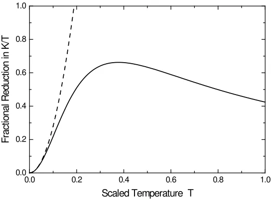
a= 0.75W was used. . . 20 2.3 Reduction in the thermal conductance divided by temperature due to
back scattering of the lowest mode, expressed as the ratio to the universal conductance divided by temperature and then scaled by aW2/δ2L, as a
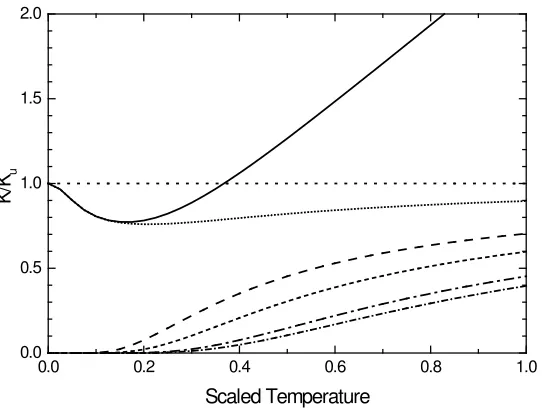
2.4 Contribution to the thermal conductance K divided by the universal value Ku from the first few modes for the ideal no scattering case, and for the rough case with scattering, as a function of the scaled tem-perature kBT /~∆: solid line—total thermal conductance for the rough surface case; dotted line and short-dotted line—conductance of mode 0 (ideal and rough); dashed line and short-dash-dotted line—conductance of mode 1 (ideal and rough); dashed-dotted line and short-dash-dotted line—conductance of mode 2 (ideal and rough). Values of the roughness parameters were a/W = 0.75 andδ/W = 0.22. . . 25 2.5 Thermal conductance relative to the universal value Ku as a function of
temperature for the ideal case (dashed line), the rough surface case (solid line), and the data of Schwab et al. (circles). The roughness parameters used were a/W = 0.75, δ/W = 0.22. . . 26
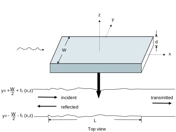
3.1 Top: Three-dimensional elastic beam with rectangular cross section. The rough surfaces are on the top, bottom, and sides. Bottom: Top view of the mathematical model of the structure actually used for the scattering calculation. . . 30 3.2 Dispersion relation for in-plane modes (solid) and flexural modes (dashed)
for a geometry ratio d/W = 0.375 and Poisson ration 0.24. The wave numbers are scaled with the widthW, and the frequencies byW/ctwith
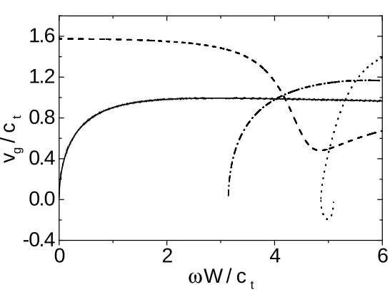
ct=pµ/ρ. . . 59 3.3 Group velocity for in-plane modes for the same parameters as Fig. (3.2):
3.4 Attenuation coefficient γmW4/˜g(0) for scattering from the two lowest
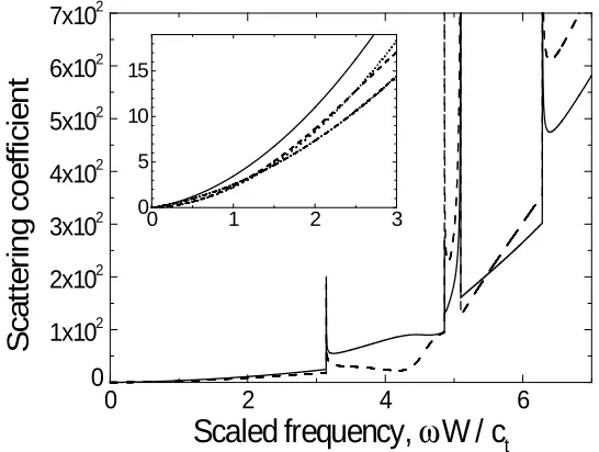
m = 0 inplane modes to any other mode as a function of scaled fre-quency ωW/ct: solid line–inplane bend mode; dashed line–compression mode. The insert shows an enlargement of the low frequency region, and compares with the analytic low frequency expressions from Table 3.2: dotted line–analytic in-plane bend mode; dash-dotted line–analytic compression mode; other lines as in the main figure. . . 62 3.5 Attenuation coefficient γmW4/˜g(0) for scattering from the two lowest
m = 0 flex modes to any other mode as a function of scaled frequency
ωp12(1−σ2)(W/d)W/cE: solid line–the flex-bend mode; dashed line–
torsion mode. The insert shows an enlargement of the low frequency region, and compares with the analytic low frequency expressions from Table 3.2: dotted line–analytic approximation for the flex-bend mode; dash-dotted line–analytic expression for the torsion mode; other lines as in the main figure. . . 63 3.6 Total scatteringP
mγmW4/g˜(0) for the in-plane modes on a log-log plot.
The dotted line shows the low frequency analytic expression from Table 3.2, and the dashed line shows a power law 4. (Note that the heights of the peaks in the plot are not significant, depending on how close the individual points, separated by 0.01 in ωW/ct, used in constructing the plot are to the mode onset frequencies where the scattering diverges.) . 64 3.7 Reduction in the thermal conductance scaled with the universal
conduc-tance Ku for the lowest in-plane modes as a function of scaled
tempera-ture T /TE with TE = ~cE/kBW: solid line–low temperature analytical
3.8 Similar to Fig. (3.7), δK/2Ku for the lowest flexural modes (torsion and flexural-bending) as a function of the scaled temperature T /TF with
TF =~cEd/kBW2. . . . 67
3.9 Attempts to fit the low temperature dataT .0.2 K using various values of aδ2: solid line–√πaδ2 = 0.1; dotted line–√πaδ2 = 0.05; dashed line– √
πaδ2 = 0.02; open circles–from the experimental data of Schwab et
al. . . 68 3.10 Thermal conductance per mode scaled with universal value Ku: solid
line–fit using roughness parametersa/W = 5.5,δ/W = 0.2, andk0W =
4.9; circles–data of Schwab et al. The dotted line shows the ideal value with no scattering. . . 70 3.11 Same as in Fig. 3.10 but showing the decrease of K/Ku from the ideal
value. . . 71 3.12 Individual mode contribution to the thermal conductance. The lowest
two flex modes and lowest three in plane modes are shown. The contri-butions toK/Ku from the four modes with zero onset frequency tend to unity at low temperatures. The higher modes only contribute at higher temperature. The modes are: dash-dotted–in-plane bending; dashed– compression; dotted–torsion; dashed-dotted-dot–out-of plane bending. The solid line shows the sum of all the mode contributions, reduced by 4Ku. Values of the roughness parameters used were a/W = 5.5,
δ/W = 0.2,k0W = 4.9, andd/W = 0.375. . . 72
5.1 A sketch of Da†0a0 E
(t) if we were able to observe the transitions of the mechanical oscillator states. . . 78
6.1 Schematics of a QMD measurement using two coupled mechanical oscil-lators. . . 83 6.2 A mechanical oscillation measurement scheme proposed by Yurke et al.
7.1 A plot of Eq. (7.73) without the stochastic component,k = 0,ν= 1 with the intitial state |1i (solid line) and with the intitial state |2i (dashed line). . . 136 7.2 Average dwelling time Tdwell of each number state between transitions.
cross: calculated from Eq. (7.74), circle: simulation results. ν = 0.02, k = 10. . . 137 7.3 A plot of a solution to Eq. (7.73) without the master equation
compo-nent, ν= 0, k= 1 with an intitially thermal state. . . 138 7.4 pnplot for a simulation of Eq. (7.73) withν = 0 for the states|0i,|1i,|2i,|3i.
The initial state is a mixed state with the average h1.63i. The figures corresponds to Fig. 7.3 (i.e., the same run). . . 139 7.5 A simulation using N0 = 1.62, ν = 0.02, and k = 5. . . 142
7.6 A simulation using N0 = 1.62, ν = 0.02, and k = 0.1. . . 143
7.7 A histogram of Da†0a0 E
(t) for a simulation t = 3000 with k = 1.5,
ν = 0.01, and N0 = 1.62. . . 144
7.8 A histogram of Da†0a0 E
(t) for a simulation t = 3000 with k = 1.5,
ν = 0.1, and N0 = 1.62. . . 144
7.9 A histogram of Da†0a0 E
(t) for a simulation t = 3000 with k = 1.5,
ν = 0.5, and N0 = 1.62. . . 145
7.10 The variation ofDa†0a0 E
(t) from integral numbers is plotted for various
k/ν ratio. It is quantified by P
N
¯ ¯ ¯ D
a†0a0
E
(t)−IntDa†0a0 E
(t) ¯ ¯ ¯ 2
/N. . . 145 7.11 T = 0.1K, N0 = 1.62, andνN/k = 0.063 with the initial state |2i. . . . 147
7.12 T = 1 K, N0 = 38, and νN/k = 0.063 with the initial state |2i. . . 147
7.13 Given the measurement current, the above figures show attempts to filter out the noise using a Butterworth filter with various band widths, for parametersk/ν = 250,N0 = 1.62. The dotted line is
D
a†0a0
E
8.1 A sketch ofn0/E2 vs.δω with various driving strengths. Curve A shows
List of Tables
3.1 Dispersion relation, group velocity, and (unnormalized) transverse mode structure for the four modes with zero frequency at zero wave vector. . 61 3.2 Scattering coefficients for the zero onset frequency modes at low
fre-quencies: c denotes compression, b denotes bend, t denotes torsion, bb denotes bend to bend scattering etc. Values are quoted for γmW4/˜g(0)
as a function of scaled frequency ¯ω = ωcE/W. For the flexural bend to bend scattering (bb) the terms in the braces in Eq. (3.72) cancel to leading order resulting in very small O(¯ω3) scattering. There is no
Part I
Quantum transport of phonons in
Chapter 1
Introduction and preliminary
calculations
Landauer’s formulation of quantum transport showed that when elastic scattering dominates, the electrical conductance can be related to the transmission coefficient of the electron waves [1]. In the ideal case of no scattering, this leads to a universal conductance that is quantized in units of e2/h at low temperatures, where e is the
electron charge andh Planck’s constant, with an additional quantum of conductance added as each channel or mode of the conductance pathway opens up. The application of similar ideas to the phonon counterpart, namely, thermal conductance, was recently derived by a number of authors [2, 3, 4], and is now recognized [5] to be related to earlier work on the entropy transport at low temperatures [6]. Rego and Kirczenow have extended the concept of the universality of the thermal conductance to particles of arbitrary statistics (anyons) [7].
The thermal conductance K of a suspended mesoscopic beam connecting two thermal reservoirs has been derived by three groups simultaneously [2, 3, 4] and the expression is
K = ~
2
kBT2
X
m
1 2π
Z ∞
ωm
Tm(ω)
ω2eβ~ω
(eβ~ω
−1)2dω, (1.1)
where the integration is over the frequency ω of the modes m propagating in the beam, ωm is the cutoff frequency of the m-th mode, β = 1/(kBT), T is the
temper-ature, kB Boltzmann constant, the factor (eβ~ω−1)
−1
n(ω), and Tm(ω) is the transmission coefficient, which equals 1 in the ideal case of
no scattering, i.e., Tm(ω) = 1. Scattering reduces the thermal conductance, and scattering of the lowest modes can reduce the conductance below the universal value,
Ku = (π2/3)k2
BT /h, at low temperatures.
In the case of electrical resistance, the chemical potential or the number of con-ducting modes can be varied at very low temperatures, giving sharp jumps between various quantized values of the resistance. On the other hand, since thermal transport by phonons necessarily requires nonzero temperatures to populate the modes of the conducting pathway, the width of the Bose distribution function smears out the quan-tization of the conductance. Only at very low temperatures, where just the modes of the conducting pathway with zero frequency at long wavelengths contribute to the thermal conductance, the quantization of the ideal conductance becomes appar-ent in a universal thermal conductance N0Ku with Ku = (π2/3)kB2T /h the universal
conductance per mode, with N0 the number of modes with zero frequency at long
wavelengths, which is four for a freely suspended elastic beam connecting the two thermal reservoirs. Note that this value of the low temperature conductance in the absence of scattering is independent of the dimensions and elastic properties of the thermal pathway.
conduc-tance decrease. We suggest that the conducconduc-tance decrease is caused by scattering due to rough surfaces. Recent advanced crystal growth technology guarantees very few impurities in the material during substrate growth, thus eliminating the possibility of impurity scattering. On the other hand, chemical etching can produce surface rough-ness on a scale of tens of nanometres, large enough to cause significant scattering.
1.1
Ideal thermal conductance
For the rest of this chapter, we consider a mesoscopic beam with rectangular cross section and its dimensions: length L, widthW, and depth d.
1.1.1
Analytical method using density of states
To evaluate Eq. (1.1), for small m, we need to evaluate the sum mode by mode, but for large m the modes become closely spaced and we can replace the sum by an integral. The density of states (i.e., the number of mode cutoffs per frequency increment) in a continuous form is
dN dω = W d 2π µ 2 c2 t + 1 c2 l ¶ ω, (1.2)
wherec2
t and c2l are transverse and longitudinal wave speeds, respectively. Let us now
evaluate the whole expression using the continuum approximation:
K = ~
2
kBT2
dW
4π2 µ 2 c2 t + 1 c2 l
¶ Z ∞
0
dωcωc
Z ∞
ωc
ω2eβ~ω
(eβ~ω
−1)2dω. (1.3)
Changing the order of integration gives
K = ~
2
kBT2
dW
4π2 µ 2 c2 t + 1 c2 l
¶ Z ∞
0
ω2eβ~ω
(eβ~ω
−1)2dω Z ω
0
dωcωc. (1.4)
Theωcintegral is easily done and then introducing the scaled frequency,y=xβ~πct/W gives
K = k
4
BT3 ~3
dW
8π2 µ 2 c2 t + 1 c2 l
¶ Z ∞
0
y4ey
(ey−1)2dy. (1.5)
The value of the last integral is 25.976. Note thatK has T3 dependence.
integral:
K = ~
2 kBT2 M X m=0 1 2π Z ∞ ωm
ω2eβ~ω
(eβ~ω
−1)2dω
+ ~
2
kBT2
dW
4π2 µ 2 c2 t + 1 c2 l
¶ Z ∞
ωM
dωcωc
Z ∞
ωc
ω2eβ~ω
(eβ~ω
−1)2dω. (1.6)
We can evaluate the integral part in the same way to give
K = ~
2 kBT2 M X m=0 1 2π Z ∞ ωm
ω2eβ~ω
(eβ~ω
−1)2dω
+k
4
BT3 ~3
dW
8π2 µ 2 c2 t + 1 c2 l
¶ Z ∞
yM
y2(y2−y2
M)ey
(ey −1)2 dy (1.7)
with yM =β~ωM, Convergence can be checked by choosing various values of M. Scaled with the universal value Ku = (π2/3) (k2
BT /h)
K Ku = π2 3 k2 BT
2π~ ~2 kBT2 M X m=0 1 2π Z ∞ ωm
ω2eβ~ω
(eβ~ω
−1)2dω
+ k
2
BT2 ~2
3dW
4π3 µ 2 c2 t + 1 c2 l
¶ Z ∞
yM
y2(y2−y2
M)ey
(ey −1)2 dy. (1.8)
This expression can be evaluated numerically. When the temperature is high enough, we can neglect the cutoff frequency and obtain an analytical expression:
K
Ku =
k2
BT2 ~2
3dW
4π3 µ 2 c2 t + 1 c2 l
¶ Z ∞
0
y4ey
(ey −1)2dy. (1.9)
1.2
Approximation methods to obtain cutoff
fre-quencies
validity range of these approximations (c.f. Fig. 1.1). We present two approximation methods: a method based on the properties of the bulk modes (§1.2.2), and a method based on thin plate theory (§ 1.2.1). Then we compare these methods with the fully numerical solution of the exact method using the “xyz algorithm” that was developed by Nishiguchi, Ando, and Wybourne [9]. This algorithm can calculate the full elastic modes, obtaining the dispersion relation of any geometry.
1.2.1
Thin plate elastic theory method
Whilst the exact solution from the 3-D elasticity theory requires full numerical ap-proach, the thin plate theory allows to obtain some analytical expressions that can be evaluated fairly easily with a lesser programming power. In addition to the com-putational reason, using the range of modes that can be approximated by the thin elastic theory, we can estimate the temperature range where the thin plate limit is applicable for a given experimental structure. This is essential information to us since our quantitative calculation of the scattering coefficient in Chapter 3 relies on the analytic expressions for the elastic modes available only in the thin plate limit. The cutoff frequencies for each mode can be determined from the dispersion relations. There are a total of four modes in a thin plate: inplane even and odd modes, and flexural even and odd modes. The dispersion relations of these four modes have been derived by Cross and Lifshitz [10]. For inplane modes,
(k2−χ2T)2tanχTW 2 + 4k
2χTχLtanχLW
2 = 0, (1.10)
4k2χTχLtanχTW 2 + (k
2
−χ2T)2tanχLW
2 = 0, (1.11)
and for flexural modes,
[ ¯K2+ (1−σ)k2]2χ−tanh(χ−W/2) = [ ¯K2−(1−σ)k2]2χ+tanh(χ+W/2), (1.12)
where
¯
K = E
3(1−2σ), µ=
E
2(1 +σ), (1.14)
cl =
s
E
ρ(1−σ2), ct=
s
E
2ρ(1 +σ), (1.15)
and E Young’s modulus, σ Poisson ratio , ρ the mass density, ω2/c2
t = k2 +χ2T =
r2(k2+χ2
L), andr=cl/ct,D=Ed3/12(1−σ2),
p
ρd/D ω= ¯K2, andχ
±=
√
k2±K¯2.
The cutoff frequencies can be obtained by solving these transcendental equations.
1.2.2
Bulk mode method
As the wavelength becomes much smaller than the dimensions of the structure, we should be able to treat the waves in terms of separate longitudinal and transverse waves in the bulk of the material, without worrying too much about the complicated standing wave transverse mode structure important for the long wavelength modes. In this regime, which we refer to as the bulk mode limit, the counting of the modes is insensitive to the details of the boundary conditions, and bulk mode approximation becomes valid. This approximation is essentially the discrete case of § 1.1.1.
For the bulk mode calculation, there are three polarizations (one longitudinal and two transverse) with propagation velocities c3l and ct, respectively, with ct as in the
2-D thin plate elasticity theory in§1.2.1, andc3l is according to 3-D elasticity theory
c3l =
s
E(1−σ)
ρ(1 +σ) (1−2σ). (1.16)
The precise details of the boundary conditions are unimportant in the mode counting for large mode numbers. If we assume standing waves in the transverse direction corresponding to zero normal derivative boundary conditions on the wave functions, the cutoff frequencies are
ωt,mn =ct
r ³mπ
W
´2
+³nπ
d
´2
for the transverse waves, and
ωl,mn =c3l
r ³mπ
W
´2
+³nπ
d
´2
, (non degenerate) (1.18)
for the longitudinal waves, withm, n= 0,1,2. . .. As mentioned before, for largem, n
we can use the continuous form for the frequency ωN of the N-th mode.
1.2.3
Comparison of the different methods
10 100 10
F
re
q
u
e
n
cy
(
ω
W
/ct
)
Mode number N
Chapter 2
Surface scattering of phonons - the
scalar model
In this chapter we use a simple scalar model for the elastic waves. The scalar model is a simple and useful tool to obtain analytical solutions, grasps the scattering behaviour, and assesses for our reason for the thermal conductance at low temperatures. This work forms the basis for a published paper [11].
y=f-(x)
y=f+(x)+W
x y
L
x=0 x=L
incident
back scattering
forward scattering
Figure 2.1: 2-D model used for calculation of the scattering of elastic waves by rough surfaces.
2.1
Scattering formalism
2.1.1
The model
The expression for the thermal conductance K of a suspended mesoscopic beam connecting two thermal reservoirs is already given in the previous chapter (Eq. (1.1)). We repeat it here for convenience
K = ~
2
kBT2
X
m
1 2π
Z ∞
ωm
Tm(ω)
ω2eβ~ω
(eβ~ω
−1)2dω. (2.1)
and refer the reader to the beginning of § 1.1 for an explanation of the notation used. The change of the thermal conductivity due to the rough surface is obtained by finding the transmission coefficient.
scattering process by considering an elastic wave propagating in the waveguide in the +x direction with wave vector k0 and entering a rough surface region of length L
(0 < x < L), where the rough boundaries are at y = W +f+(x) and y = f−(x) so
that the roughness is characterized by the functions f±(x). We assume that the top
and the bottom roughness functions are uncorrelated, and that f±(x) is small and
is differentiable. The incident wave Ψin interacts with the rough surface, is scattered
into other modes Ψsc, and leaves the rough region. The total field Ψ is the sum of
the incident field and the scattered field
Ψ = Ψin+ Ψsc. (2.2)
Our task is to find an expression for Ψsc and hence calculate the transmission
coeffi-cients. As said before, we do this by using Green functions.
2.1.2
Green function method
2.1.2.1 Scattering amplitude and Green function
In terms of fields, the S-matrix formulationS = 1+iT can be written with an incident field and scattering field. The matrix 1 corresponds to the incident field as explained previously andT matrix corresponds to a scattered field. The easiest and clearest way to obtain the scattered field, Ψsc, is to use a Green function. The Green function is a
solution to the Helmholtz equation with a point source. The description of scattering in terms of scattering amplitudes and that in terms of Green functions are equivalent in a far-field regime [12].
2.1.2.2 Green function
We start with the Helmholtz equation for a scalar wave at frequency ω
where K is ω/c with c the wave speed. Define the Green function as a solution to the point sources
∇2G(x, y;x0, y0) +K2G(x, y;x0, y0) = −δ(x−x0)δ(y−y0) (2.4)
with (x0, y0) the source coordinates and (x, y) the observation coordinates. It is
con-venient to define G(x, y;x0y0) such that it satisfies Neumann boundary conditions at
the smoothed boundaries, y= 0, W
∂G/∂n|y=0,W = 0, (2.5)
where ˆn is the outward-pointing normal to the surface. We then project the physical boundary conditions at the rough surfaces onto the smoothed boundaries to calculate the scattering.
Multiplying Eq. (2.3) by G(x, y;x0, y0) and Eq. (2.4) by Ψ(x, y) then subtracting
one from the other, and integrating over a volume bounded by the position of the smoothed surfaces yields the result of Green’s theorem
Ψ (x, y) = Z
smooth
dx0∂Ψ (x
0, y0)
∂n0 G(x
0, y0;x, y)
±
Z
x→±∞
dy0
·
∂Ψ (x0, y0)
∂x0 G(x
0, y0;x, y)
−Ψ (x0, y0)∂G(x
0, y0;x, y)
∂x0
¸
, (2.6)
where the first integral is the integration along the smoothed edges and the second over the distant ends taken atx→ ±∞, each with its proper sign. We have used the boundary condition Eq. (2.5) for G to eliminate a second term in the first integral.
We now need to calculate the Green function. The Green function G(x, y;x0, y0)
satisfies Eq. (2.4). Using the completeness relation, the right hand side can be written
− 1
2π
Z ∞
−∞
eik(x−x0)dkX
n
where φn is the normalized transverse eigenfunction for smooth boundaries
φn=Nncosχny (2.8)
with χn =nπ/W, n = 0,1,2, .., and Nn the normalization factor: Nn =p2/W for
n 6= 0 and Nn = p1/W for n = 0. The Green function is then given by Fourier transforming
G(x, y;x0, y0) = 1
2π
Z ∞
−∞
dkX
n
eik(x−x0)
φn(y)φn(y0)
k2+ (nπ/W)2−K2. (2.9)
The k integral in Eq. (2.9) is now evaluated by contour integration. The poles cor-responding to propagating waves at k = pK2−(nπ/W)2 for K > nπ/W must be
given infinitesimal imaginary parts ±iε to yield outgoing waves. We then have
G(x, y;x0, y0) =X
n
ieikn|x−x0|φn(y)φn(y0)
2kn
, (2.10)
where
kn=
p
K2−n2π2/W2 nπ/W < K
ipn2π2/W2−K2 nπ/W > K . (2.11)
The second term in Eq. (2.6) is just the incoming wave Ψin(x, y) as will be
dis-cussed below, so that
Ψsc(x, y) =
Z
smooth
dx0∂Ψ (x
0, y0)
∂n0 G(x
0, y0;x, y). (2.12)
In Appendix A.2, it is shown that evaluating the second term in Eq. (2.6) results in the incident field.
2.1.3
Boundary perturbation
the smoothed surface appearing in the integral by expanding about the stress-free rough surface [13]. We will present the calculation for the rough lower surface, and simply double the scattering probabilities assuming uncorrelated roughness on the two surfaces.
Firstly, we express the unit normal vector as
ˆ
n=−yˆ+f−0 (x) ˆx. (2.13)
Then we impose the Neumann boundary condition at y=f−(x)
µ
−∂Ψ (x, y)
∂y +f
0 −(x)
∂Ψ (x, y)
∂x
¶¯ ¯ ¯ ¯
y=f−(x)
= 0. (2.14)
Now we expand this equation abouty = 0 in terms off− and retain only terms that
are first order in f andf0. This gives the normal derivative at the smooth surface up
to first order in f, f0 as
∂nΨ (x, y)|y=0 =
£
f0
−∂xΨ (x, y)−f−∂y2Ψ (x, y)
¤¯ ¯
y=0. (2.15)
Thus the scattered field to first order in the roughness amplitude is
Ψsc(x, y)'
Z
dx0G(x0, y0;x, y)£
−f−(x0)∂y20Ψin(x0, y0) +f−0 (x0)∂x0Ψin(x0, y0)
¤¯ ¯
y0=0,
(2.16) where we can replace the field appearing in the integral by the incident field Ψin at
this order.
It is now straightforward to insert the explicit expression for the Green function Eq. (2.10) to calculate the scattering from a normalized incident wave entering in the
m-th mode Ψin(x, y) = Ψm(x, y) = Nmcos (χmy)eikmx:
Ψsc(x, y)'
Z
dx0X
n
iN2
nNm
2kn cos (χny)e
ikn|x−x0|£f
−(x0)χ2m+ikmf−0 (x0)
¤
eikmx0.
2.1.4
Scattered field
Outside the scattering region, Eq. (2.17) takes the form for the scattered field
Ψsc(x→+∞, y)
=X
n
eiknxcos (χny)
Z ∞
−∞
dx0iN
2
nNm
2kn
£
χ2mf−(x0) +ikmf−0 (x0)
¤
ei(km−kn)x0, (2.18)
Ψsc(x→ −∞, y)
=X
n
e−iknxcos (χny)
Z ∞
−∞
dx0iiN
2
nNm
2kn
£
χ2mf−(x0) +ikmf−0 (x0)
¤
ei(km+kn)x0, (2.19)
giving the forward scattered field and back scattered fields respectively. The terms inf0
− can be simplified by integration by parts.
Z ∞
−∞
dx0if−0 (x0)kmei(km∓kn)x0 =km(km∓kn) ˜f
−(km∓kn), (2.20)
where ˜f− is the Fourier transform off−, i.e. f˜− =
R∞
−∞dx 0f
−eikx
0
, and we have used the fact that the roughness is confined to 0< x < L, so thatf−(±∞) = 0.
Now using K =pχ2
m+k2m, we get
Ψsc(x→ ±∞, y) =
X
n
iNnNm
2kn f˜−(km∓kn)
¡
K2∓knkm¢
Ψn(x, y), (2.21)
for the forward and backward scattered waves, expressed as a sum over normalized waves Ψn.
2.1.5
Roughness characterisation
Previously we have defined two surface profile functions byf±(c.f. Fig. 2.1) Since they
are rough surface functions, we treat them statistically. Thenf+(x) and f−(x) have
correlation function are
hf(x)i= 0, (2.22)
hf(x)f(x0)i=δ2g(|x−x0|), (2.23)
where δ is the root mean square (rms) roughness and g(|x−x0|) is the roughness
correlation function, which only depends on the distance betweenxandx0. h idenotes an average over the ensemble of realizations of the function. The correlation for Fourier transform of this function Df˜(k) ˜f∗(k)E is
D ˜
f(k) ˜f∗(k)E=
¿Z
dxf(x)eikx
Z
dx0f(x0)e−ikx0
À
= Z Z
dxdx0hf(x)f(x0)ieik(x−x0)
= Z
dx0
Z
d(x−x0)δ2g(|x−x0|)eik(x−x0)
=δ2L
Z
d(x−x0)g(|x−x0|)eik(x−x0)
= ˜g(k)δ2L, (2.24)
where ˜g(k) is the roughness correlation function in Fourier space and Lis the length of the rough surface is the flat surface. Thus the roughness fluctuation is characterised by
¿ ¯ ¯ ¯f˜−(k)
¯ ¯ ¯
2À
=δ2g˜(k)L, (2.25)
where δ2g˜(k) is the Fourier transform of the surface roughness correlation function
with δ the roughness amplitude. As we mentioned before, we have assumed that the roughness function, ˜f−, is stochastic (spatial not temporal) and treat it statistically.
We also assume that the correlation function of the roughness function is Gaussian
g(x) =e−x2/a2
with the correlation lengtha. Since the Fourier transform of a Gaussian is a Gaussian, we obtain
˜
g(k) = √πaexp
·
−a
2k2
4 ¸
Now we apply this correlation function to calculate the scattering probability using the result from Eq. (2.21). Lett±n,m be the scattering amplitude from modemto±n,
where the plus sign is for forward scattering and the minus sign is for back scattering. Then from Eq. (2.21) we have the scattering amplitude
t±n,m =
iNnNm
2kn
¡
K2∓knkm¢ ˜
f−(km∓kn). (2.27)
To calculate the transmission coefficient appearing in the expression for the thermal conductance we need the energy flux scattering probabilities σ±n,m, given by
multi-plying |tn,m|2 by the ratio of the group velocities
σ±n,m =
kn km
|t±n,m|2
®
. (2.28)
The angular brackets denote the average of the rough surface. This finally gives
σ±nm =
N2
nNm2
4knkm
£
K2∓knkm¤2
δ2˜g(km∓kn)L , (2.29)
where ˜g is the correlation function in Fourier space ˜g(km∓kn) = ¿
¯ ¯ ¯
˜
f−(km∓kn)
¯ ¯ ¯
2À
.
2.1.6
Thermal conductance
To calculate the thermal conductance we must recognize that not all scattering pro-cesses decrease the heat transport. A wave entering in mode m has four possible outcomes: after the scattering events it may stay in mode m propagating forward; it may be converted to mode n also propagating forward; it may stay in mode m but propagating backward (call this mode −m); and finally it may be converted to mode
n and propagating backward (call this−n). The former two cases do not change the heat transport, since each mode at frequency ω contributes the same amount to the conductance. The two back-scattering events do reduce the heat transport, however. Thus the backward scattering rate σ−n,m contributes to the reduction of the thermal
un-0 1 2 3 4 0
1 2 3 4
S
ca
le
d
A
tt
e
n
u
a
tio
n
C
o
e
ff
ic
ie
n
t
Reduced Frequency ω/∆
Figure 2.2: Scaled attenuation coefficients (W4/δ2aL)|σ
−n,m|2 as a function of
re-duced frequency,ω/∆ where ∆ =πc/W withcthe velocity of the waves: solid—from modem = 0 to mode−n,n = 0. . .3 and dashed—modem to mode−m,m= 1. . .3. A value of the roughness correlation length a= 0.75W was used.
changed. We therefore define the conductance attenuation coefficient per unit length of the rough surface waveguide as γm ≡(2/L)P
nσ−n,m. The factor of two accounts
for scattering off the top surface. We have
γm =X
n
(K2+k
nkm)2 knkm
√πN2
nNm2δ2a
2 e
−a2(kn+km)2/4
. (2.30)
The conductance attenuation coefficient γm gives the exponential decay rate of the wave in mode m, so that over a length L the transmission is
Tm =e−γmL. (2.31)
2.31) into Eq. (2.1):
K = ~
2
kBT2
X
m
1 2π
×
Z ∞
ωm
dω ω
2eβ~ω
(eβ~ω
−1)2 exp[− X
n
(K2+knkm)2
knkm
N2
nNm2
√
πδ2aL
2 e
−a2(k
n+km)2/4].
(2.32)
The contributions to the conductance attenuation coefficients per unit length γm
for the first few modes are shown as a function of the mode frequency in Fig. 2.2. A scattering correlation length ofa/W = 0.75 was used in the figure. The backscattering amplitude from the lowest mode (mode 0) to its reverse is
γ00(ω, a, δ) = 2π
1
2aδ
2
W2
ω2
c2e
−a2ω2/c2
. (2.33)
This expression is finite for all frequencies. It has a maximum at a frequencyω =c/a
depending on the roughness correlation length, with a peak value of order (δ2/aW2).
The higher modes have a divergent back-scattering proportional to (ω−ωm)−1 at the
cutoff frequenciesωm. In addition eachγmhas a contribution diverging as (ω−ωn)−1/2
at the onset of the n-th mode. These divergences are due to the flat spectrum at the mode cutoff frequencies, and will also be found in the full elastic wave calculation.
At low enough temperatures only the lowest mode with k0 = ω/c contributes
0.0 0.2 0.4 0.6 0.8 1.0 0.0
0.2 0.4 0.6 0.8 1.0
F
ra
ct
io
n
a
l R
e
d
u
ct
io
n
in
K
/T
Scaled Temperature T
Figure 2.3: Reduction in the thermal conductance divided by temperature due to back scattering of the lowest mode, expressed as the ratio to the universal conductance divided by temperature and then scaled by aW2/δ2L, as a function of temperature
scaled by kBT /~∆.
may be replaced by unity, exp[−a2ω2/c2]'1. This leads to
K
T '
π2k2
B
3h
"
1−8π
9/2
5
δ2aL
W4
µ
kBT ~∆
¶2#
, (2.34)
where ∆ = πc/W is the spacing between the mode cutoff frequencies. Thus at low temperatures, the conductance divided by temperature should show a quadratic temperature decrease with an amplitude depending on the combination of roughness parameters aδ2/W3.
2.2
Comparison with the experiment of Schwab
et
al.
with width W = 160 nm and length L = 1µm. In the experimental geometry the width varied along the length to provide smooth junctions with the reservoirs. This was done to eliminate scattering off abrupt changes in the geometry. We use the width at the narrowest point as our estimate of the size of the structure. For the length we use the length of the central portion over which the width is constant. Since the length only occurs in the combination δ2L, changing the value of L used
will only change the fitted value ofδ. We use a wave propagation speed c= 8250 m/s which is the reciprocal average of the velocity of longitudinal and transverse elastic waves in silicon nitride.
The roughness parameters are not known a priori. As a first attempt, we might try to estimate the combination aδ2L/W4 from a quadratic fit to the decrease in
the thermal conductance data at low temperatures, Eq. (2.34). This would give the value aδ2L/W4 ∼ 0.05. However, from Fig. 2.3 we see that the quadratic low
temperature fit is only good up to about a quarter of the temperature of the maximum backscattering of the first mode. If we estimate this temperature from the minimum in the measured conductance, we find that the data does not extend to low enough temperatures to provide a reliable fit, and so this value can only be used as an order of magnitude. In fact our “best fit” (see below) over temperatures up to 1 K corresponds to a valueaδ2L/W4 about a factor of 4 larger.
It is interesting to use this value of the roughness parameters to estimate the strength of the scattering of the higher modes. For example, for the first mode, with cutoff frequency ∆, and at a wave vector π/W corresponding to a frequency √2∆, we find for the backscattering into the same mode
γ1(k1 =π/W)L∼16 exp ¡
−π2a2/W2¢
. (2.35)
The scattering increases for smaller wave vectors, diverging at onset as shown in Fig. 2.2. Remember that the transmission amplitude is e−γ1L. This means that the
To fit the higher temperature data using Eq. (2.32) we will find that we need a value of a comparable to W. Although this strongly reduces the value of γ1(k1 = π/W),
there remain frequency ranges where the scattering of this mode and other modes is strong. An interesting consequence is that a significant fraction of the thermally excited phonons at temperatures of order 1 K are predicted to be localized in the experiments of Schwab et al., with a localization length less than the length of the bridge. Unfortunately, in this regime the estimate of the contribution to the conduc-tance from these modes predicted by our lowest order scattering calculation, will not be accurate. Kambili et al. [14] have used a similar model in a numerical investiga-tion of the effect of surface roughness on the mode propagainvestiga-tion. The scattering of scalar waves in waveguides with rough surfaces has been also investigated numerically by other workers [15, 16] in a diffusive region - a transition regime between ballistic regime and localised regime.
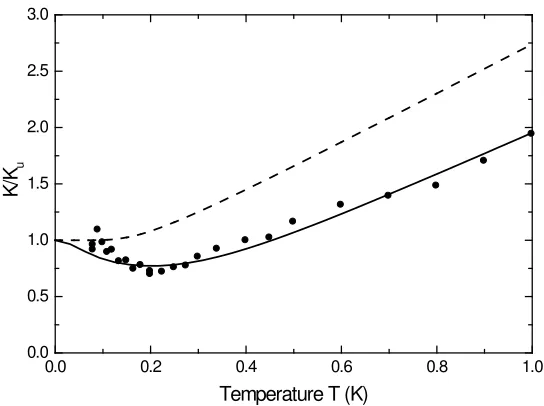
From Fig. 2.3 we can suggest two mechanisms that might account for the observed minimum in the dependence of K/T on temperature. The first mechanism ascribes the minimum in K/T to the behaviour of the first mode alone, as plotted in Fig. 2.3. The upturn in K/T arises from the reduced scattering of the lowest mode as the wave vectors of the important modes increase with temperature. The second mechanism supposes that the scattering of the lowest mode is responsible for the decreasing K/T at low temperatures, but that the subsequent increase is from the thermal excitation of the higher modes. For our “best fit” values of a, δ (see below) the results are summarized in Fig. 2.4. The picture is quite complicated, with both the reduced scattering of the lowest mode and the thermal excitation of the higher modes contributing to the rise in K/T with increasing temperature. Furthermore, due to the strong scattering of the higher modes near their cutoff frequencies, these modes become important in the transport at a higher temperature than would be estimated simply from their cutoff frequencies.
0.0 0.2 0.4 0.6 0.8 1.0 0.0
0.5 1.0 1.5 2.0
K
/Ku
Scaled Temperature
Figure 2.4: Contribution to the thermal conductanceK divided by the universal value
Ku from the first few modes for the ideal no scattering case, and for the rough case with scattering, as a function of the scaled temperature kBT /~∆: solid line—total thermal conductance for the rough surface case; dotted line and short-dotted line— conductance of mode 0 (ideal and rough); dashed line and short-dash-dotted line— conductance of mode 1 (ideal and rough); dashed-dotted line and short-dash-dotted line—conductance of mode 2 (ideal and rough). Values of the roughness parameters werea/W = 0.75 andδ/W = 0.22.
The roughness parameters a/W = 0.75 and δ/W = 0.22 (so that aδ2L/W4 = 0.23)
0.0 0.2 0.4 0.6 0.8 1.0 0.0
0.5 1.0 1.5 2.0 2.5 3.0
K
/Ku
Temperature T (K)
Figure 2.5: Thermal conductance relative to the universal value Ku as a function of
temperature for the ideal case (dashed line), the rough surface case (solid line), and the data of Schwab et al. (circles). The roughness parameters used werea/W = 0.75,
δ/W = 0.22.
There are small but systematic differences at very low temperatures, where the conductance is dominated by the lowest modes, and the theory should be most ac-curate. The discrepancy suggests that we are overestimating the scattering at long wavelengths. A roughness spectrum ˜g(k) ∼ k2e−a2k2/4
Chapter 3
Detailed analysis of surface
scattering effects - the elastic
model
3.1
From a scalar model to an elastic model
In this chapter we again calculate the effect on the low temperature thermal conduc-tance of the scattering of the thermal phonons by surface roughness, but this time, using elastic waves. In the last chapter, we described the scattering in waveguides with rough surfaces via a scalar wave equation. However, this does not accurately cap-ture the low frequency modes of interest at low temperacap-ture. For example, the scalar model predicts a linear dispersion at small wave vectors. In fact the dispersion rela-tions of the modes are different, with two of the four modes with zero long-wavelength frequency having a quadratic dispersion at small wave vectors, rather than the linear one given by the simple scalar theory.
To understand the experimental results quantitatively, a more accurate treatment of the vibrational waves is needed. At low temperatures, the wavelengths of the ther-mally excited modes are large compared with the atomic spacing, and so a treatment based on the equations of macroscopic elasticity theory is appropriate. Blencowe [4, 18] has considered the scattering of elastic waves in a thin plate waveguide with rough surfaces1, but prior to our work, the scattering of elastic waves confined in a
1Blencowe has considered a semi-infinite thin plate. In his case, the out-of-plane mode is a
beam-like wave guide with rough surfaces has not been considered.
At the end of the last chapter, we noted the apparent discrepancy between the results of the scalar model with a simple assumption for the nature of the surface roughness and the data by Schwab et al. [8] below a temperature of 0.1 K: the data seemed to show a delay of the onset of scattering as the temperature increased that was not predicted by the model. However, since the scalar model does not properly account for the properties of the elastic waves, it was not clear whether this discrepancy is due to inadequate modelling of the surface roughness or a flaw in the description of the waves themselves. To resolve this matter, and to obtain a more accurate account of the scattering of the waves by rough surfaces, we develop a theory based on the full elasticity equations, and use this to calculate the thermal conductance at low temperatures. This work forms the basis for three published papers [19, 20, 21].
In § 3.2, the scattering of elastic waves confined to a beam of rectangular cross section with rough surfaces is calculated using the full three dimensional elasticity theory. We use a Green theorem approach, and calculate the scattering coefficient to quadratic order in the amplitude of the surface roughness. These results are quite general, but are rather intractable for further progress, since the structure of the modes in an elastic beam cannot be determined in closed form. Thus in§3.3 we reduce the expressions to a thin plate limit to provide a closed form for the displacement fields, and to obtain analytical expressions for the scattering behaviour. In § 3.4 the general behaviour of the scattering and the effect on the thermal conductance is analysed in detail, using a simple description of the surface roughness, to investigate the physical consequences of the novel features of the elastic waves. In § 3.5 we use our theory to attempt to fit the data of Schwab et al. [8] using more realistic descriptions of the surface roughness. A number of the more difficult issues that arise in the elasticity theory are described in appendices.
Although our main interest is the scattering of thermally excited vibrational waves in mesoscopic systems at low temperatures, the formulation of the surface scattering
is quite general, and can be applied to other situations, such as the scattering of mechanically excited modes in macroscopic samples, for example.
3.2
General formalism
3.2.1
The model
The geometry we consider in this chapter is a 3-D freely suspended elastic beam, which we call the bridge, connecting two thermal reservoirs. We will consider a beam of rectangular cross section of dimensions width W (in the y direction) and depth d
(in the z direction). Mesoscopic structures are often produced lithographically from epitaxially grown material. We choose a convention that the depth is the dimension in the growth direction, and the width in the lithographically defined transverse direction. We define the length of the rectangular beam of nominally uniform cross section as L. In practice the bridge may be joined to the reservoirs smoothly, by a portion of continuously growing width, to eliminate or reduce the scattering of the vibration modes off a sharp junction. We will suppose that the scattering by roughness is important only in some narrower portion of length L.
To actually perform the scattering calculation we imbed the rough beam of length
L in an infinite beam of the same cross section but with smooth surfaces outside of the region of length L, Fig. 3.1. In the previous chapter, we have defined the rough surface boundaries in y-direction to be y = f−(x, z) and y = W +f+(x, z). In
this chapter, we shift the coordinate such that the boundaries in y-direction will be symmetrical about the origin. Thus the mathematical calculation is the scattering of a wave incident from x = −∞ on a rough portion of the beam with surfaces at
y = ±W/2±f1(x, z) and at z = ±d/2±f2(x, y), with the height functions f1,2,
defining the roughness, nonzero only in a finite region 0< x < L. Forward scattering is evaluated from the intensity of waves as x →+∞, and backward scattering from the intensity of waves asx→ −∞.
x z
y
d
L W
transmitted incident
reflected
y= W 2
-Top view - f1 (x,z)
y= W 2 + + f1 (x,z)
Figure 3.1: Top: Three-dimensional elastic beam with rectangular cross section. The rough surfaces are on the top, bottom, and sides. Bottom: Top view of the mathe-matical model of the structure actually used for the scattering calculation.
to the one used for the scalar model in the previous chapter.
The displacement field u away from any sources satisfies the wave equation:
ρ∂t2ui =∂jTij, (3.1)
where ρ is the mass density, and
Tij =Cijkl∂kul (3.2)
is the stress tensor field with Cijkl the elastic modulus tensor. The subscript i runs over the three Cartesian coordinates, we use the symbol ∂x to denote the derivative
∂/∂x etc., and repeated indices are to be summed over. The displacement field satisfies stress-free boundary conditions at the surfaces
Tijnj|S = 0, (3.3)
harmonic time dependence at frequency ω, Eq. (3.1) becomes
ρω2ui+Cijkl∂j∂kul= 0. (3.4)
We approximate the material of the system as an isotropic solid. Then the elastic modulus tensor is
Cijkl =λδijδkl+µ(δikδjl+δilδkj), (3.5)
where λ and µare Lam´e constants (µ is also the shear modulus)
λ=Eσ/(1 +σ)(1−2σ), µ=E/2 (1 +σ) (3.6)
with E Young’s modulus andσ the Poisson ratio.
Even in a rectangular beam geometry the displacement fields in the propagating modes yielded by these equations are complicated, and cannot be found analytically. The modes can be grouped into four classes according to their signature under the parity operations y → −y and z → −z. Some modes show regions of anomalous dispersion where the group velocitydω/dkis negative: these regions require a careful examination of the notions of “forward” and “backward” scattering for the waves. The lowest frequency mode of each class has a frequency that tends to zero at small wave number. These four modes are the only ones excited at low enough temperature, and are the ones contributing to the universal thermal conductance. The structure of these modes at small wave numbers is simple and can be calculated using familiar macroscopic arguments of elasticity theory: they are the compression, torsion, and two orthogonal bending modes.
We define a Green function Giq(x,x0;t, t0) to satisfy the wave equation with a
source term −δiqδ(x−x0)δ(t−t0), and Γ
ijq to be the corresponding stress
It is convenient to introduce the frequency space version of the Green function
Giq(x;x0;t, t0) =
Z dω
2πGiq(x;x
0;ω)e−iω(t−t0)
, (3.8)
with a similar expression defining Γijq(x,x0;ω). Inserting G, Γ, and the source term
into Eq. (3.4) gives
ρω2Giq(x,x0;ω) +∂jΓijq(x,x0;ω) = −δiqδ(x−x0), (3.9)
where xis the observation coordinate and x0 is the source coordinate.
Equations (3.4) and (3.9) lead to Green’s theorem expressing the displacement field at frequency ω in terms of a surface integral
uq(x) =
Z
S0
£
n0jTij(x0)Giq(x0,x;ω)−n0jui(x0) Γijq(x0,x;ω)
¤
dS0. (3.10)
We are free to choose any closed integration surface S0. One choice is to use the
physical rough surface thereby eliminating the first term in Eq. (3.10) due to the boundary condition Eq. (3.3). However, the resulting integration over the rough surface is not easy. Instead, we integrate over the smoothed surfaces at y =±W/2 and z = ±d/2 and impose the boundary conditions on the Green function to be stress-free on these smoothed surfaces
Γijqnj|S = 0, (3.11)
together with cross sections atx0 → ±∞to close the surface.
The total field u can be written as the sum of incident and scattered waves
3.2.2
Incident and scattered fields
Using Green’s theorem we have expressed the displacement field at frequency ω in terms of the surface integral
uq(x) =
Z
S0
£
n0jTij(x0)Giq(x0,x)−n0jui(x0) Γijq(x0,x)
¤
dS0. (3.13)
Eq. (3.13) involves the integration over a closed surface S0, which we have chosen to
be the smooth boundaries together with the cross sections at x0 → ±∞. We show
that the integration over the sections at ±∞simply yields the incident field uin
q, and
this allows us to deduce the expression for the scattered field as an integration over the side surfaces. To deduce this result, we first need to derive what are known as reciprocity relations for the elastic modes. We follow Auld’s approach [22] to derive reciprocity relation. Remember that for x→ ±∞ the surfaces are smooth, so we are interested in the modes of the ideal beam here.
Let u(r) and u(s) be the displacement fields for modes r and s in the ideal beam,
and T(r), T(s) the corresponding stress tensor fields. The modes satisfy the wave
equation at frequency ω, so that
ρω2u(ir)+∂jTij(r) = 0. (3.14)
Multiply the first equation byu(is)∗ and the complex conjugate of the second byu(ir), subtract the two equations, integrate over a volume of the beam between x=x1 and
x=x2, and finally use the divergence theorem to find
Z
S
h
ui(s)∗Tij(r)−ui(r)Tij(s)∗iˆnjdS = 0, (3.15)
where the integral is over the surface bounding the volume, consisting of the sides of the beam between x1 and x2, and the sections at x1 and x2. The integrations
and T(r) = T¯(r)(y, z)eikrx, with kr the wave number of mode r at frequency ω, etc.
Then Eq. (3.15) reduces to
¡
1−ei(kr−ks)(x1−x2)¢
Z Z h
φi(s)∗T¯ix(r)−φi(r)T¯ix(s)∗idydz = 0, (3.16)
and the integral is independent of x. Unless the prefactor is zero, this shows us that the integral over the section must be zero, and so
Z Z h
ui(s)∗Tix(r)−u(ir)Tix(s)∗i dydz = 0, kr 6=ks. (3.17)
This is one version of the reciprocity relations.
For our purposes it is more convenient to express the condition for the reciprocity integral to be zero in terms of the group velocity rather than the wave number. To do so, we need to consider the dispersion curves. The condition for the reciprocity integral to be nonzero, kr = ks for modes r, s at the same frequency ω, actually implies r and s are the same mode, so that in fact vg(r) = vg(s). The only other
possibility is that r and s are modes with dispersion curves that cross at frequency
ω,k =kr=ks. However only modes of differenty, z parity signatures can cross, and
then the integration over the section for these different modes in Eq. (3.17) is again zero. Thus we can rewrite the reciprocity relation as
Z Z h
ui(s)∗Tix(r)−u(ir)Tix(s)∗i dydz= 0, vg(r) 6=v(gs). (3.18)
If r and s are the same mode, the integral is related to the energy flux and hence to the group velocity (see Eq. (3.25))
Z Z
dydz³u(ir)∗Tij(r)−ui(r)Tij(r)∗´= 2iρωvg(r). (3.19)
We now use Eqs. (3.18, 3.19) to evaluate the contributions to Eq. (3.13) from the integrations over the sections at x0 → ±∞.
Green’s function pairG,Γconsist of modes us(x0)∗ withv(gs) <0 since herex0 > xfor
any finitex. On the other hand the field pair u,T are made up of the incident wave, and waves scattered from the roughness at finite x, and so consist of modes ur(x0)
with v(gr) >0. The integral in Eq. (3.13) over the section at x0 → ∞ is therefore the
sum of terms involving R R h
u(is)∗Tix(r)−u(rr)Tix(s)∗
i
dydz with v(gr) and vg(s) of opposite
sign. All these terms are zero by Eq. (3.18), and so there is no contribution from the section at x0 → ∞.
Similar arguments apply to the section atx0 → −∞. The Green function is made
up of modes with vg >0. The scattered component of the field u consists of modes
with vg <0, and there is no contribution to the integral over the section from these modes. On the other hand the incident waveuin is modeu
m withv(gm)>0, and there
is the single term with vg(n) = vg(m) surviving in the sum over modes in the Green
function. Using Eq. (3.19) the integral just givesu(qm)(x). So the integration over the
sections atx0 → ±∞on the right-hand side of Eq. (3.10) just givesuin
q. On the other
hand, in the integration over the smoothed surfaces aty=±W/2 and z =±d/2 the second term in the integrand vanishes due to Eq. (3.11). Thus we find the expression for the scattered field
usc
q (x) =
Z
dS
£
n0
jTij(x0)Giq(x0,x;ω)
¤
dS0, (3.20)
with the surface S the smoothed surfaces y =±W/2 and z =±d/2. The stress field
Tij on the smoothed surface is evaluated by expanding about its value on the rough
surfaces, where Eq. (3.3) applies. Writingu =uin+usc then leads to Eq. (3.20).
3.2.3