Robustness, Adaptation, and Learning in Optimal Control
Thesis by Ivan Papusha
In Partial Fulfillment of the Requirements for the Degree of
Doctor of Philosophy
California Institute of Technology Pasadena, California
2016
c
2016
Acknowledgments
First and foremost, I would like to thank my incredible advisor, Prof. Richard Murray, for his guidance and support during my graduate school years. He helped me clarify ideas, and gave me great freedom to pursue the best ones. Despite his full schedule, Richard always made time for me. He has forever earned a place in the back of my mind as the voice that asks questions like “why?” “what is the big picture?” and “suppose you could do this. . . ”
Huge thanks also go to my thesis committee, Profs. John Doyle, Joel Burdick, and Eugene Lavretsky. Their great courses and sharp insight into robust control, robotics and estimation, and adaptation got me excited about the intersection between control theory and engineering. I was extremely privileged to have the geniuses of my field, right here at Caltech, helping to answer my questions and giving advice. I also want to acknowledge my officemates and close friends S. You, A. Swaminathan, K. Shan, as well as my peers and col-laborators J. Fu, U. Topcu, E. Wolff, S. Livingston, I. Filippidis, K. Shankar, M. Horowitz, S. Farahani, C. McGhan, N. Matni, and V. Jonsson for many insightful discussions.
I want to give a special thanks to Prof. Vijay Kumar and his group at the University of Pennsylvania, especially M. Pivtoraiko and R. Ramaithitima, for graciously providing the facilities and expertise with the quadrotor experiments that appear in this thesis.
Of course, I would not be anywhere without my amazing family. Great thanks go to my mom, grandma, and little sister Katya, for providing support and encouragement from across the continent.
Abstract
Recent technological advances have opened the door to a wide variety of dynamic control applications, which are enabled by increasing computational power in ever smaller devices. These advances are backed by reliable optimization algorithms that allow specification, syn-thesis, and embedded implementation of sophisticated learning-based controllers. However, as control systems become more pervasive, dynamic, and complex, the control algorithms governing them become more complex to design and analyze. In many cases, optimal con-trol policies are practically impossible to determine unless the state dimension is small, or the dynamics are simple. Thus, in order to make implementation progress, the control designer must specialize to suboptimal architectures and approximate control. The major engineering challenge in the upcoming decades will be how to cope with the complexity of designing implementable control architectures for these smart systems while certifying their safety, robustness, and performance.
Contents
Acknowledgments v
Abstract vii
List of Symbols xii
1 Introduction 1
2 Lyapunov Theory 7
2.1 Conserved and dissipated quantities . . . 7
2.2 Lyapunov’s stability theorem . . . 10
2.3 Robust control . . . 18
2.3.1 Linear differential inclusions . . . 18
2.3.2 Quadratic stability margins. . . 21
2.4 Fundamental variational bounding ideas . . . 23
2.5 References . . . 26
3 Model Predictive and Approximately Optimal Control 27 3.1 Online optimization for control . . . 27
3.2 Box constrained quadratic programming . . . 29
3.2.1 Primal-dual path following algorithm . . . 30
3.2.2 Taking advantage of structure . . . 32
3.3 Discrete-space approximate dynamic programming . . . 32
3.3.1 Bounds on the value function . . . 32
3.3.2 Setup . . . 33
3.3.3 Bellman operator . . . 34
3.3.5 Bound optimization by linear programming . . . 35
3.3.6 Approximation guarantees and limitations . . . 37
3.3.7 Optimization with unknown transition probabilities . . . 38
3.3.8 Example: Gridworld . . . 40
3.4 Continuous-space approximate dynamic programming . . . 41
3.4.1 Example: Linear quadratic dynamics with bounded control . . . 43
3.5 Extensions . . . 45
3.6 References . . . 45
4 Automata Theory Meets Approximate Dynamic Programming 47 4.1 Introduction . . . 47
4.2 Problem description . . . 49
4.3 Product formulation . . . 51
4.4 Lower bounds on the optimal cost . . . 54
4.4.1 Linear quadratic systems . . . 55
4.4.2 Nonlinear systems . . . 57
4.5 Examples . . . 58
4.5.1 Linear quadratic systems with halfspace labels . . . 58
4.5.2 More complex specification . . . 60
4.6 Conclusion . . . 63
5 Adaptation and Learning 65 5.1 Introduction . . . 65
5.2 Robust adaptation . . . 69
5.3 Dynamic estimation . . . 73
5.3.1 Least squares estimator . . . 73
5.3.2 Constrained estimator . . . 75
5.3.3 Equality constrained least squares estimator . . . 76
5.3.4 Learning example: Finite measure estimation . . . 77
5.4 Case study: Controlling wing rock . . . 79
5.4.1 Open loop limit cycle . . . 80
5.4.2 Robust design . . . 81
6 Networked Adaptive Systems 85
6.1 Introduction . . . 85
6.1.1 Preliminaries . . . 86
6.2 Problem setting . . . 87
6.2.1 Parameter estimator dynamics . . . 87
6.2.2 Persistence of excitation . . . 88
6.2.3 Proof of Theorem 4 forp= 1 . . . 94
6.3 Interpretations and related problems . . . 98
7 Conclusion 107 7.1 Summary and contributions . . . 107
7.2 On the title . . . 108
7.3 Current and future directions . . . 109
Appendix A Proof of Theorem 4 for p >1 113
List of Symbols
Notation Meaning
R,Rn,Rm×n real numbers,n-dimensional vectors, andm×nmatrices
C,Cn,Cm×n complex numbers,n-dimensional vectors, and m×nmatrices
j the imaginary unit,√−1
1 the vector of all ones,i.e., (1, . . . ,1)∈Rn
Sn symmetricn×nmatrices {X∈Rn×n|X=XT}
Sn+ positive semidefinite matrices{X∈Sn|zTXz≥0 for allz6= 0}
Sn++ positive definite matrices{X∈Sn|zTXz >0 for allz6= 0} P 0,P ≻0 same asP ∈Sn+,P ∈Sn++, dimension taken from context P K Q,P ≻KQ P−Q∈clK, andP −Q∈intK, where K is a convex cone
Tr(M) trace of a matrixM ∈Rn×n,i.e.,Pni=1Mii
λmax(P),λmin(P) maximum, minimum eigenvalue of a matrixP ∈Sn
σmax(M), σmin(M) maximum, minimum singular value of a matrixM ∈Rm×n
Co(S) convex hull of the setS⊆Rn, given by
Co(S) =
( k X
i=1
θixi |xi ∈S, θi≥0, i= 1, . . . , k, k
X
i=1 θi = 1
)
Lp signalsu:R+→Cn withkukp =
R∞
0 ku(τ)kpdτ
1/p <∞, 1≤p≤ ∞
kuk 2-norm for vectors,L2-norm for signals,σmax(u) for matrices
H∞ Hardy space onCn+
Ex expected value of a random variablex
P(A) probability of an eventA
ˆ
θ(t),y(t)ˆ estimate at timet of a parameterθ∈Rnθ, and output y∈Rny ˜
θ(t),∆θ(t) parameter estimation error ˆθ(t)−θ∈Rnθ ˜
Chapter 1
Introduction
From its classical engineering roots in the 1930s–40s, increasing mathematization in the 1950s–60s, through to the present day, the discipline of control has been progressive in its adoption of computational tools and algorithms. The Nyquist criterion, Bode and Nichols plots, Kalman filter, KYP lemma, LMIs, and convex optimization are all tools designed by control theorists, or imported from other fields to solve an engineering question. But instead of giving a specific answer, more often than not these theoretical tools lead to a procedure, which the control designer—in their quest for practical implementation—must execute, check and recheck, abandon, resurrect, tune, and check once more. The final proof is in the pudding. After all, the goal is to control dynamical systems.
This reliance on algorithms starkly conflicts with the standard practice in mathematics and physics, where definite answers reign supreme. A true 17th century mathematician would never be satisfied until a closed-form solution to a problem has been obtained. Only a formula, or an equation, a concept—something simple—into which someone could substitute facts and figures, would make them happy. Whereas a mathematician wants to tell youwhat
orwhy something is, a control theorist would be more interested inhow to make it happen. These algorithmic tools help researchers and decision makers working in a variety of multidisciplinary fields, such as biology and medicine, transportation, and earth sciences. By making use of a strong tradition in modeling and abstraction of physical systems, they are able to solve problems they could not before. Control theory has the right pedigree to help contextualize some of the toughest “squishy” and “applied” questions, because it lies at the intersection of engineering and mathematics, and has an obsession with both intellectual rigor and practicality.
computers, and ever better optimization algorithms. As our world becomes increasingly automatized, engineers are faced with very real societal needs to create complex and opti-mized automatic systems that affect more and more people. Meanwhile, these systems must operate safely, robustly, and with high performance. This means that practice continues to outpace rationale. In fact, the late Jan Willems predicted the influx of optimization technology as the next “big thing” in control. In his autobiographical essay, he wrote
. . . MPC is an area where essentially all aspects of the field, from modeling to optimal control, and from observers to identification and adaptation, are in synergy with computer control and numerical mathematics [Wil07].
MPC stands for Model Predictive Control, a particular kind of optimization-based con-trol method that comes from the chemical process community. Its main idea is very simple:
1. model the system
2. using the model, make a plan from now until a timeT later (with optimization) 3. execute the first portion of the plan, and let the system evolve
4. go to step 2.
Model Predictive Control is arguably one of the most compelling, highly performant, and most broadly applicable tools control theory has to offer. For example, it has the ability to incorporate constraints on the input and state. It neatly ties together observers and controllers. It can be extended to nonlinear, hybrid, stochastic, and machine learning systems. It has beautiful links to dynamic programming, and encompasses all of LQR, LQG, and Kalman filtering.
However, the very thing that makes control relevant, namely feedback, appears in MPC in an indirect way. Somewhere between steps 3 and 4, a measurement of the true system must take place. Unlike classical control—where this measurement process appears centrally with the notions of signals, closed-loop poles, and small gain theorems—optimization-based control treats stability through foreign concepts liketerminal costs,control-Lyapunov func-tions, invariant sets, and tubes. Furthermore, the notion of feedback is made even more difficult to track by the inherent discrete time (or epoch) nature of the optimization-based control.
In other words, the frequency domain currency is no good here. This makes sense, because frequency domain tools primarily operate on linear systems, while an optimization-based control strategy is inherently nonlinear. Thus, there is a very clear disconnect: on the one hand, control designers want to use MPC because it is so simple and works so well. On the other hand, they are wary because when applied without care to convergence and stability issues, MPC can fail spectacularly—often at a great (physical) cost.
To help alleviate some of these concerns, this thesis argues that the right way to think about optimization-based control is through bounds on the Lyapunov, or energy, func-tion (Chapter 2). Lyapunov bounds help answer quesfunc-tions about robustness, adaptation, and learning through algorithms, specifically convex optimization algorithms. In so doing, some systems concepts are brought back to the optimization-based setting. Specifically, we enlist the help ofadaptive androbust control to design approximate adaptive- or robust-by-construction control methods, which must be implemented online as convex optimization problems (Chapters 3–4).
We must use algorithms to find tractable bounds, because for all but the simplest linear systems, exact Lyapunov functions are notoriously difficult to compute. Ways to provide useful upper and lower bounds have frequently come up as a theme in the past. Although hints at the idea can probably be traced back to Bellman [Bel57], the most illuminating reference is a two-part series on dissipation theory by Willems [Wil72a, Wil72b], in which he describes the notion of an energy storage function and a dissipation inequality. The storage function is bounded below by the available storage and above by the required supply. Since then, many researchers have used these ideas to develop bounds-based control and estimation policies.
pervades our approach. More importantly, these bounding techniques lead to efficiently computed approximate policies, depending on the type of bound employed. By using bounds instead of the true Lyapunov function, we give up some optimality for efficient synthesis or guarantees about safety. Of course, if useful bounds cannot be obtained or implemented, usually because the class of Lyapunov function candidates is not rich enough, we must remain agnostic about the applicability of these methods. However, in many cases results speak for themselves—as shown when Lyapunov bounding techniques are applied to formal methods and hybrid systems (Chapters 3–4).
Closely related to the Lyapunov thinking that led to the success of adaptive control are notions of identifiability that can be exported to other fields, such as communication networks and machine learning. Part of this thesis concentrates on novel notions of identifi-ability and persistence of excitation. Classical schemes in system identification and adaptive control often rely on persistence of excitation to guarantee parameter convergence, which may be difficult to achieve with a single agent and a single input. However, by adding communication to the mix, we show that it is possible to obtain parameter convergence even if no single agent employs a persistently exciting input (Chapters 5–6).
Summary of contributions. Chapter 2 grew out of a course that my advisor graciously let me develop and teach during Spring 2015. While the main ideas date back to Lya-punov [Lya92], and are (by now) fairly standard in nonlinear control, the notation is up-dated for the modern mathematical palate, often following the language of linear matrix inequalities [BEFB94, Boy08] and dissipation inequalities [Wil72a, Wil72b]. Chapter 3 reviews MPC, and presents recent directions for fast implementation, referencing ideas com-ing from various software implementations. These optimization tools are then combined with approximate dynamic programming to obtain Lyapunov bound based policies. The closest works are [BT96, Ran99, dFR03, WOB14], however the applications and exam-ples are new. Chapter 4 is a novel application of bounds-based techniques to approximately solve hybrid and temporal logic constrained problems, based on the paper:
Chapter 5 switches gears to adaptation and learning by describing robust adaptive con-trol in the language of optimization and Lyapunov bounds developed in the previous chap-ters. This chapter explores novel reformulations and makes connections between learning theory and adaptive control. The fundamental departure frome.g., [LW13, IF06] is to view adaptive control not just as the result of a clever zeroing of dissipation terms in a Lyapunov argument, but rather as the implementation of a specific (continuous-time or discrete-time) algorithm for solving a constrained convex optimization problem online. This view is made more explicit in Chapter 6, which introduces a new concept of networked adaptive systems by specializing to a specific subspace parameter consensus constraint and implementing a gradient flow. In this networked setting, we derive an identifiability criterion and adapta-tion algorithm that trades off time and space, resulting in provable parameter convergence even without persistence of excitation. This last chapter is based on the paper:
[PLM14] I. Papusha, E. Lavretsky, and R. M. Murray. Collaborative system identification via parameter consensus. In American Control Conference (ACC), pp. 13–19. June 2014.
Not directly referenced in this thesis are the following additional publications:
[HPB14] M. B. Horowitz, I. Papusha, and J. W. Burdick. Domain decompo-sition for stochastic optimal control. In IEEE Conference on Decision and Control (CDC), pp. 1866–1873. 2014.
[PM15] I. Papusha and R. M. Murray. Analysis of control systems on symmetric cones. InIEEE Conference on Decision and Control (CDC), pp. 3971–3976. December 2015.
Chapter 2
Lyapunov Theory
2.1
Conserved and dissipated quantities
In this section we set out notation by discussing autonomous dynamical systems of the form
˙
x(t) =f(x(t)), x(0) =x0, (2.1)
where x(t) ∈ Rn is the system state at time t, and f : Rn → Rn is a function that corresponds to the (infinitesimal) direction of evolution of the state: given a state space location x ∈ Rn, the quantity f(x) is a tangent vector that points in the direction of the trajectory, see Figure 2.1. We assume that the initial value problem (2.1) has a unique solution x(t) for all t≥ 0. This can be ensured, for example, if f is a globally, uniformly Lipschitz continuous function of its argument, see e.g., [CL55, Per01].
x f(x)
Rn
Figure 2.1: Schematic of general autonomous system ˙x=f(x(t)).
form. However, we would still like to quantitatively analyze the stability or dissipativity of the system (2.1) without reference to specific trajectories of f. An energy orLyapunov
function allows us to describe the behavior of the system (2.1) in a quite general way. For the remainder of this section, letV :Rn→Rbe a given real-valued function of state space.
Level sets. Given a real scalarα∈R, theα-level set Lα of V is the set
Lα ={z∈Rn|V(z) =α}.
Conserved quantities. We say that V is a conserved quantity if it is constant along trajectories of (2.1). The quantity V is conserved if its time derivative does not change,
d
dtV(x(t)) =∇V(x(t))
Tf(x(t)) = 0, (2.2)
for allt. If V is a conserved quantity, then trajectories of (2.1) stay in level sets of V. To see why, suppose V(x(0)) =α. Integrating ˙V along the trajectories of (2.1) gives
V(x(t)) =V(x(0)) +
Z t
0 ˙
V(x(τ))dτ =α+
Z t
0 ∇
V(x(τ))Tf(x(τ))
| {z }
=0
dτ
=α,
for all t≥0. Thus if x(0)∈ Lα and V satisfies the condition (2.2), then x(t) ∈Lα for all t≥0.
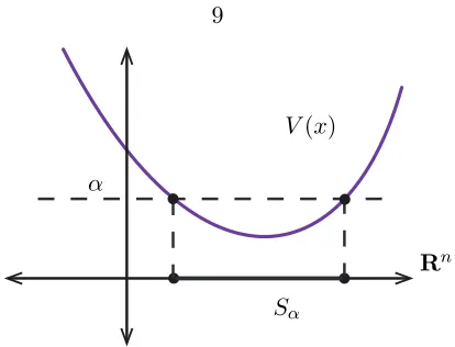
Sublevel sets. Given a real scalar α∈R, theα-sublevel set Sα of V is the set
Sα={z∈Rn|V(z)≤α}.
V(x) α
Rn
Sα
Figure 2.2: Sublevel setsSα given an energy functionV(x).
Dissipated quantities. We say thatV is adissipated quantity if it is nonincreasing along trajectories of (2.1). The quantity V is dissipated if its time derivative is nonpositive,
d
dtV(x(t)) =∇V(x(t))
Tf(x(t))≤0, (2.3)
and strictly dissipated if its time derivative is negative, d
dtV(x(t)) =∇V(x(t))
Tf(x(t))<0, (2.4)
for allt. A key property of dissipated quantities is that trajectories of (2.1) stay in sublevel sets ofV. To see why, suppose V(x(0)) =α. Integrating ˙V along the trajectories of (2.1) gives
V(x(t)) =V(x(0)) +
Z t
0 ˙
V(x(τ))dτ =α+
Z t
0 ∇
V(x(τ))Tf(x(τ))
| {z }
≤0
dτ
≤α,
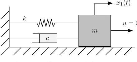
Example 2.1 Spring-mass-dashpot. The system illustrated in Fig 2.3 below has the linear dynamics
x˙1
˙
x2
| {z }
˙
x(t)
=
0 1
−k m − c m
x1
x2
| {z }
f(x(t))
,
where x1(t) is the signed displacement of the mass from its equilibrium position,x2(t) = ˙x1(t)
is its velocity,mis the mass,kis the spring constant, and cis dashpot constant.
m
u= 0 k
c
x1(t)
Figure 2.3: Spring-mass-dashpot system.
Define V(x1, x2) = 12kx21+12mx22 as the total energy (kinetic plus potential) of the mechanical
system. The energy derivative is
˙
V(x1, x2) =
kx1
mx2 T
0 1
−k m − c m
x1
x2
=−cx22.
The total energyV is conserved ifc= 0, and dissipated if c >0. Note that by our definition, the total energy is not necessarily strictly dissipated, becauseV(x1,0) = 0 for allx1.
2.2
Lyapunov’s stability theorem
Lyapunov’s insight. We should note that the conservation and dissipation conditions (2.2), (2.3), and (2.4) can be interpreted in two ways. First, we can think ofV(x(t)) as a quantity that depends on a given trajectoryx(t). The time derivative ˙V(x(t)) is therefore computed indirectly through x(t). This way of thinking, however, is not particularly useful, because it requires knowing the full trajectory x(t).
conditions (2.2), (2.3), and (2.4) as
∇V(x)Tf(x) = 0, ∀x∈Rn (2.2′)
∇V(x)Tf(x)≤0, ∀x∈Rn (2.3′)
∇V(x)Tf(x)<0, ∀x∈Rn\ {0} (2.4′)
to stress that V is a function on the state space Rn, rather than of a specific trajectory x(t). Thus whether or not V is conserved or dissipated can be concluded by checking the conditions (2.2′), (2.3′), or (2.4′).
The power of this small shift in thinking, widely attributed to Lyapunov’s 1892 the-sis [Lya92] has not gone unnoticed in the dynamical systems community. As we will see, the power of this shift lies in an ability to quantify stability, optimality, and robustness of control policies. Lyapunov is arguably the principal enabler of modern control.
Generalized energy. A function V : Rn → R is positive definite if it satisfies the following conditions:
• V(x)≥0 for allx∈Rn, • V(x) = 0 if and only ifx= 0, • All sublevel sets ofV are bounded.
A positive definite function is a kind of generalized energy for the system. As Lyapunov’s famous result asserts, the existence of a strictly dissipated generalized energy is a sufficient condition for the stability of the system.
Example 2.2 The quadratic function V(x) = xTP x is positive definite if and only if the
matrixP is a positive definite matrix,P ≻0.
Theorem 1 (Lyapunov, 1892). Suppose there is a function V :Rn→R such that
• V is positive definite (generalized energy)
Proof. Suppose x(t) 6→ 0 as t → ∞. Since V is a dissipated, nonnegative quantity, the conditionsV(x(t))≥0 and ˙V(x(t))≤0 together mean thatV(x(t)) is a monotone, bounded function of t, therefore V(x(t)) → c1 > 0 as t → ∞ for some positive constant c1. In particular,c1 ≤V(x(t))≤V(x(0)) =c2 for all t≥0. Take
C={z∈Rn|c1 ≤V(z)≤c2}.
Since C is a compact subset of Sc2, which excludes a neighborhood of the origin, andV is
strictly dissipated, we have supz∈CV˙(z) =−γ <0 for some positive constant γ. But the energy at time tis given by
V(x(t)) =V(x(0)) +
Z t
0 ˙ V(x(τ))
| {z }
≤−γ
dτ ≤c2−γt,
which is negative for large t, leading to a contradiction.
Example 2.3 Consider the linear system ˙x=Ax, whereA∈Rn×n, and defineV(x) =xTP x,
whereP =PT
∈Rn×nis a given symmetric matrix. The derivative along trajectories of ˙x=Ax
is given by
˙
V(x) = ˙xTP x+xTPx˙
= (Ax)TP x+xTP(Ax) =xT(ATP+P A)x.
Thus, we conclude the following:
• V is positive definite if and only ifP ≻0.
• V is strictly dissipated if and only if ATP+P A ≺0.
We can restate Lyapunov’s theorem in the linear setting as follows: if there exists a matrix
P ≻0 withATP+P A≺0, then all trajectories of ˙x=Axconverge to the origin ast→ ∞.
system; see, e.g., [Kra63, LSW96]. One example is linear systems, for which it is easy to see that a quadratic Lyapunov function is sufficient to prove stability.
Example 2.4 Converse Lyapunov result for linear systems. LetQ=QT ≻0 be any positive
definite matrix and let ˙x=Axbe a (Hurwitz) stable system. Let
P =
Z ∞
0
eATτ
QeAτdτ,
which is well defined because all eigenvalues ofAhave negative real part. Consider the quadratic Lyapunov functionV(x) =xTP x.
˙
V(x(t)) =x(t)T(ATP+P A)x(t) =x(t)T
AT
Z ∞
0
eATτ
QeAτdτ +
Z ∞
0
eATτ
QeAτdτ A
x(t) =x(t)T
Z ∞
0
d dt
n
eATτ
QeAτodτ
x(t) =−x(t)TQx(t)
for any trajectory x(t) of the system. Thus the quantity V is positive definite and strictly dissipated. The matrix P, also known as a Gramian, satisfies the Lyapunov equationATP+
P A+Q= 0.
Example 2.5 Certificate of instability. Let ˙x = Ax be an autonomous linear system and suppose there exists a function V(x) =xTP xwith P 60 such that ATP+P A0. Then A
is not (Hurwitz) stable.
To see this, note that the condition ATP +P A 0 implies that all trajectories of the
au-tonomous system ˙x=AxsatisfyV(x(t))≤V(x(0)) for allt≥0, because
V(x(t))−V(x(0)) =
Z t
0
˙
V(x(τ))dτ
=
Z t
0
x(τ)T(ATP+P A)x(τ)
| {z }
≤0
dτ ≤0.
But since P 6 0, there exists a vector w such that V(w) <0. Setting the initial condition
x(0) =w, we have
V(x(t))≤V(w)<0, for all t≥0.
Graphical interpretation. We can interpret Lyapunov’s theorem graphically by plotting the level and sublevel sets of the functionV. A schematic view is shown in Figure 2.4. Here, the solid line denotes a particular level setLα ={z∈Rn|V(z) =α} for a given scalarα, and the shaded area inside is the sublevel set Sα ={z ∈Rn |V(z)≤α}. If V is positive definite, then Sα is bounded. The arrowed line corresponds to a particular trajectoryx(t). For a given state x, the inner product between the vectors ∇V(x) andf(x) determines whether a trajectory throughxwill enter the appropriate level or sublevel set. For example, if the inner product is zero (∇V(x)Tf(x) = 0,V is conserved), then a trajectory throughx will follow the level set ofV corresponding toV(x) =α. If the inner product is nonpositive, (∇V(x)Tf(x)≤0,V is dissipated), then the trajectory throughxcannot escape the sublevel set Sα. Finally, if the inner product is strictly negative (∇V(x)Tf(x) < 0, V is strictly dissipated), then the trajectory throughx must enter intSα.
x
∇V(x) f(x)
V(x) <α V(x)
>α V(x) =
α
Figure 2.4: Graphical interpretation of Lyapunov’s theorem.
As the following example illustrates, some care must be taken to ensure strict dissipation when considering the stability of a system.
Example 2.6 Non-strict dissipation. If it can only be concluded that ˙V(x) ≤ 0 but not ˙
V(x)<0, then trajectories can “hide” in the zero-dissipation set
Z={z∈Rn|V˙(z) = 0}.
Let ˙x = Ax be an autonomous linear system and consider V(x) = xTP x with the specific
constants
A=
0 −1
1 0
, P =
1 0
0 1
In this case,V is positive definite, and dissipated (but not strictly dissipated), becauseATP+
P A = 0. The zero-dissipation set is Z = R2. In fact, this “center” system has circular trajectories that do not approach the origin, unless they already start there.
Decay rate. IfV(x) =xTP xis positive definite and dissipated with the further restriction that ˙V(x)≤ −2αV(x), then trajectories of (2.1) decay exponentially with rate at leastα,
lim t→∞e
αtkx(t)k 2 = 0.
In this case, the scalarαis aLyapunov exponent for the system. To see why the decay rate is at least α, recall Gr¨onwall’s inequality, which states
˙
h(t)≤g(t)h(t) for all t∈(a, b) =⇒ h(t)≤h(a) exp
Z t
a
g(τ)dτ
for all t∈(a, b).
Applying Gr¨onwall’s inequality to V(x(t)) gives the bound
V(x(t))≤V(x(0)) exp
−
Z t
0 2α dτ
,
which means x(t)TP x(t)≤x(0)TP x(0)e−2αt for all t≥0. Therefore,
kx(t)k2 ≤
s
σmax(P) σmin(P)k
x(0)k2e−αt, for all t≥0.
Evidently, such a Lyapunov function certifies that the decay rate is at leastα.
Region of attraction. Lyapunov functions can also be used to estimate regions of attrac-tion by comparing the regions of state space over which the Lyapunov funcattrac-tion is strictly dissipated against the Lyapunov function’s sublevel sets. Define the region of attraction
R={x0∈Rn| lim
t→∞x(t) = 0}
as the set of initial conditions in (2.1) for which the trajectory through that initial condition approaches the origin. Next, define the strict dissipation set
Trajectories starting at a pointx0 ∈ Dwith initial energyV(x0) =αmust initially stay within Sα, because V is dissipated within D. If Sα happens to contain a point outside D, then a trajectory through that point can gain energy and escape Sα, because dissipation of V is only guaranteed within D. However, if Sα is entirely within D, then no trajectory can escape Sα. Therefore, Sα⊆ R is an inner approximation of the region of attraction R if it can be shown thatSα ⊆ D. Depending on the problem, it may be easier to show that Sα ⊆ D (for example, by semidefinite programming) than to compute R explicitly. See Example 2.7 and Figure 2.5 for an illustration.
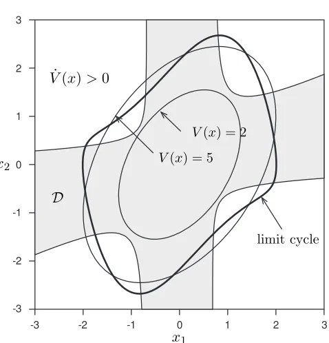
Example 2.7 Van der Pol oscillator. Consider the dynamics
˙
x1=−x2
˙
x2=x1+ (x21−1)x2,
which are locally stable about the equilibrium (0,0). The region of attractionRcorresponding to this equilibrium is enclosed by the limit cycle (Figure 2.5). Using a quadratic Lyapunov function of the formV(x) =xTP x,
V(x) =
x1
x2
T
1.5 −0.5
−0.5 1
| {z }
P
x1
x2
, ATP+P A=−I≺0,
we can form an ellipsoidal estimate of Ras follows. First, we determine the strict dissipation regionD. Then, we search for the maximum scalar αfor which the sublevel setSα is entirely
contained inD. In this case, the largest such sublevel set corresponds toS2.25. Therefore,S2.25
is an inner approximation ofR.
0 1 2 3 -1
-2 -3
0
-1
-2
-3 1 2 3
limit cycle
x1 x2
˙
V(x)>0
V(x) = 2
V(x) = 5
D
Figure 2.5: Van der Pol region of attraction estimate. The strict dissipation set (shaded) is
D={z|V˙(z)<0} ∪ {0}, with the largest ellipsoidal sublevel set contained inDgiven bySα={z|
V(z)≤2.25}. The true region of attractionRis the area enclosed by the limit cycle.
Theorem 2. For the state space system x˙ =Ax, V(x) =xTP x, and
˙
V(x) =xT(ATP +P A)x=−xTQx,
if P ≻0 and Q ≻0, then x(t) →0. Conversely, if x˙ =Ax is (Hurwitz) stable, then there exists P ≻0 and Q≻0 to prove it.
Results for linear systems are also typically global. Consider a linear system ˙x=Ax. For a quadratic Lyapunov functionV(x) =xTP x, the energy sublevels are (possibly degenerate) ellipsoids,
Sα ={z∈Rn|zTP z≤α}. If the system is stable, the dissipation sets are all ofRn,
D={z∈Rn|V˙(z) =zT(ATP+P A)z≤0}.
Since Sα ⊆ D = Rn for all α, we conclude that state space systems are either globally stable, or not globally stable.
study of linear systems to be viewed as the study of invariant ellipsoids and the sublevels of an appropriate quadratic function, or more usefully, of the associated quadratic form. Many textbooks have been devoted to this subject [FK96, Son98, Kha02], and it is not our intention to reproduce that work here. The interested reader is referred to the text-book [Kha02] for a general treatment of linear and nonlinear stability theory, and to [DP00] for a more control theoretic spin. This thesis builds on these works, but specifically uses the conventions and notation of [BEFB94, FK96].
2.3
Robust control
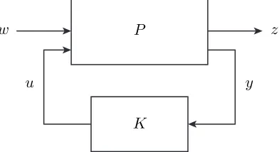
2.3.1 Linear differential inclusions
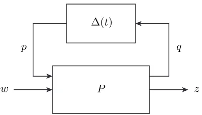
P
K
u y
w z
Figure 2.6: Robust controller synthesis.
A linear system with unknown or uncertain parameters can be described as a state space model
˙
x=A(t)x+Bu(t)u+Bw(t)w z=Cz(t)x+Dzu(t)u+Dzw(t)w x(0) =x0,
(2.5)
where x∈Rnx is the state, u∈Rnu is the control input,w ∈Rnw is an exogenous input, and z ∈ Rnz is the regulated output. The goal of a typical robust control problem is to choose a control input u as a function of a measured output y that minimizes some cost index that relates the inputs, outputs, and disturbances. For simplicity we will consider
is the assumption that the model matrices obey
A(t) Bu(t) Bw(t)
Cz(t) Dzu(t) Dzw(t)
∈Ω, for all t,
for a given description of the set Ω⊆R(nx+nz)×(nx+nu+nw). Such a description is called a Linear Differential inclusion (LDI).
LTI systems. The set Ω might consist of a single element,
Ω =
A Bu Bw
Cz Dzu Dzw
,
in which case the system is known fully. It is still subject to disturbances w, however the design procedure for robust controllers for LTI systems is considerably simplified, at most requiring the solution of linear (Lyapunov) or quadratic (Riccati) matrix equations.
Polytopic systems. In this case, the set Ω might be described by the vertices of a polygon,i.e.,
Ω =Co
A1 Bu,1 Bw,1
Cz,1 Dzu,1 Dzw,1
, . . . ,
AL Bu,L Bw,L
Cz,L Dzu,L Dzw,L
.
Optimal controller synthesis with a common Lyapunov function for polytopic model uncer-tainties usually requires semidefinite programming.
Norm-bound systems. A very useful uncertainty class consists of model descriptions of the form
Ω =nA˜+ ˜B∆(I−Dqp∆)−1C˜ | k∆k2≤1
o , (2.6) where ˜ A=
A Bu Bw
Cz Dzu Dzw
, B˜ =
Bp
Dzp
, C˜=hCq Dqu Dqw
i
.
The set Ω is the image of the matrix unit ball under the matrix linear-fractional mapping
and is well-posed provided DTqpDqp ≺I. The norm-bound model uncertainty corresponds to a linear state-feedback perturbation ∆(t) being applied to an LTI system as shown in Figure 2.7.
P ∆(t)
p q
w z
Figure 2.7: Norm-bound perturbation.
The specific way this perturbation is applied to (2.5) is interpreted as follows. We can rewrite the uncertain dynamics (2.5) subject to a norm-bound feedback perturbation as the dynamical system,
˙
x=Ax+Bpp+Buu+Bww q=Cqx+Dqpp+Dquu+Dqww z=Czx+Dzpp+Dzuu+Dzww p= ∆(t)q, k∆(t)k2 ≤1
x(0) =x0.
(2.8)
In this state-space description (2.8), a signalq is “picked off” from the original LTI dynam-ics (2.5). That signal is then fed through a gain-bounded block to generate an uncertain signalp= ∆(t)q. The signalpis then applied back to the dynamics (2.5). To see that (2.7) is the correct mapping for the norm-bound perturbation, we rewrite (2.8) in matrix form,
˙ x z q =
A Bu Bw Bp Cz Dzu Dzw Dzp Cq Dqu Dqw Dqp
x u w p
The last row of (2.9) can be eliminated. With p= ∆(t)q, the last row reads
q=hCq Dqu Dqw
i x u w
+Dqp∆(t)q
= ˜C
x u w
+Dqp∆(t)q, (2.10)
so if (I −Dqp∆(t)) is invertible for all t, we can determine q from (2.10) by taking the inverse,
q = (I−Dqp∆(t))−1C˜
x u w
. (2.11)
Substituting (2.11) back into (2.9) gives
x˙
z
=A˜+ ˜B∆(t)(I−Dqp∆(t))−1C˜
x u w ,
which gives the uncertainty description (2.6). The well-posedeness assumption
I−Dqp∆(t)≻0, k∆(t)k2 ≤1 for allt,
restricts the domain of the mapping (2.7) so the set Ω is convex. By making use of the norm bound k∆(t)k2 ≤ 1, equivalently the map (2.7) is well posed if and only if DTqpDqp ≺ I. This assumption is often satisfied by removing the dependence ofqonpby settingDqp = 0.
2.3.2 Quadratic stability margins.
remaining quadratically stable.
Guaranteed LQR margins. Consider the state feedback system
˙
x=Ax+B∆u u=Kx,
(2.12)
whereK =−R−1BTP is an LQR gain, andP ≻0 satisfies the algebraic Riccati equation
ATP+P A−P BR−1BTP +Q= 0
for given matricesQ≻0,R≻0. Assume thatRis diagonal and the matrix ∆∈Rnu×nu is a diagonal multiplicative perturbation to the input of a nominal system. The system (2.12) is quadratically stable with Lyapunov function V(x) = xTP x if the matrix ∆ satisfies ∆ii≥1/2 for all i= 1, . . . , nu.
To see why, we can use the Riccati equation to show that
˙
V(x) =xT(P B(R−1−R−1∆T −∆R−1)BTP−Q)x <0 for allx6= 0
providedR−1−R−1∆T −∆R−10, which happens if ∆ is diagonal with ∆
ii≥1/2. This corresponds to a classical lower gain margin of
20 log10(1/2) =−6dB
and an upper gain margin of∞. Thus, LQR is robust to 1/2 gain reduction and unbounded gain amplification in each input channel.
LQR margin shaping. We can view the LQR state feedbacku = (I+ ∆)Kx with an uncertain additive feedback perturbation by rewriting (2.12) as
˙
x=Ax+Buu+Bpp q=Cqx
p= ∆q, k∆k2 ≤α,
where Bp = Bu and Cq = K are fixed, and the nominal control input is u = Kx. If the input uncertainty is norm-bounded byα(and not necessarily diagonal), withk∆k2 ≤α, we can ask the question of for which α is (2.13) quadratically stable. Equivalently, with the Lyapunov function V(x) =xTP x, we ask when is the quadratic form
˙ V(x) =
x
p
(A+BuK)
TP+P(A+B
uK) P Bp BT
pP 0
x
p
≤0,
for all (x, p) satisfying (2.13). From theS-procedure, we conclude that (2.13) provided the matrix inequality
P ≻0, τ ≥0,
(A+BuK)TP +P(A+BuK) +τ α2CqTCq P Bp
BpTP −τ I
0
is feasible. Substituting the Riccati equation and K=−R−1BTP, this is equivalent to
P ≻0, τ ≥0,
−Q−P BuR−
1(I−τ α2R−1)BT
uP P Bu BT
uP −τ I
0,
which is feasible providedα2 ≤λ
min(R)/λmax(Q−1/2P BTP Q−1/2).
2.4
Fundamental variational bounding ideas
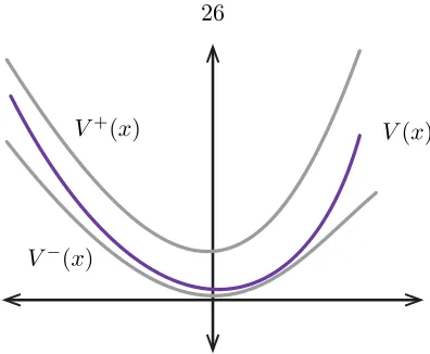
One of the most powerful applications of Lyapunov theory to control lies in two very simple bounds. One of these bounds gives an upper bound to the Lyapunov function, and the other gives a lower bound. Although they differ only in the sense of inequality, and are obtained in effectively the same way, these two bounds lead to very different interpretations of the Lyapunov function.
To see how this kind of bounding works, we consider the autonomous system
˙
x(t) =A(t)x(t), x(0) =x0, (2.14)
One might think of the choice of A(t) as being made nondeterministically by an adver-sarial nature, in which case the specific value of A(t) is unknown beyond the uniqueness and set membership constraints, or by thedesigner, in which case the valueA(t) is perhaps determined by a control algorithm. Let
J =
Z ∞
0
ℓ(x(t))dt
denote the cost of a given trajectory x(·) satisfying (2.14), where ℓ(x)≥0 for all x ∈Rn. Note thatJ might be infinite if the system (2.14) is unstable.
Now suppose there exists a continuously differentiable Lyapunov functionV+:Rn→R that satisfies
V+(x)≥0, V˙+(x)≤ −ℓ(x), (2.15) for all x∈Rn and for all A(t) ∈Ω. Then for a fixed x0, the quantity V+(x0) is an upper
bound onJ. To see this, we integrate along the trajectory
V+(x(T))−V+(x(0)) =
Z T
0 ˙
V+(x(t))
| {z }
≤−ℓ(x(t)) dt
≤ −
Z T
0
ℓ(x(t))
| {z }
≥0 dt
≤ −
Z ∞
0
ℓ(x(t))dt=−J,
where the first inequality follows from (2.15), and the second from the nonnegativity of the loss functionℓ. Therefore, we have
J ≤V+(x(0))−V+(x(T))≤V+(x0), for all T,
because V+(x(T)) is nonnegative for all T. ThusV+(x0) is an upper bound on the worst-case cost of the trajectory for any valid choice of the valuesA(t) that nature might make.
In fact, we have the variational inequality
J ≤Jwc = inf
V+satisfies (2.15)V
+(x
0), (2.16)
case valueJwc, a quantity obtained by minimizingV+(x0) over all functionsV+that satisfy the condition (2.15). Thus if we are able to compute the infimum in (2.16), and it is finite, then we have a quantifiable measure of the robustness of the cost with respect to the choice of A(t) at every time instant t. It is sometimes possible to quantify this robustness given the description of the set Ω alone. For example, if Ω is consists of a single Hurwitz matrix element, then (2.14) must be stable, and J is no more than the initial energy. However, if nature wanted to be devious, it might pick A(t) ∈argmaxA∈ΩV˙+(x(t)) as a function of x(t) to make the cost as close toJwc as possible.
On the other hand if the Lyapunov function satisfies the reverse inequality
V−(x)≥0, V˙−(x)≥ −ℓ(x), (2.17)
for all x∈Rn and for all A(t)∈Ω, then the same chain of inequalities leads to
J ≥V−(x0)−V−(x(T)),
for allT. Now suppose that the state trajectoryx(·) is asymptotically stable, andV−(0) = 0, then asT → ∞we haveV−(x(T))→0. In other words,V−(x0) is alower, or performance bound for any stabilizing choice of the valuesA(t). Similarly, we have the variational bound
J ≥Jperf= sup V−satisfies (2.17)
V−(x0), (2.18)
therefore no stabilizing A(t) can ever achieve the performance limitation Jperf. To get a sequence that gives a small cost, a control designer might chooseA(t)∈argminA∈ΩV˙−(x(t)) as a function ofx(t) to make the cost as close to the performance limit Jperf as possible.
V(x) V+(x)
V−(x)
Figure 2.8: Upper and lower bounds on a Lyapunov function.
2.5
References
Chapter 3
Model Predictive and
Approximately Optimal Control
3.1
Online optimization for control
In the previous chapter, we introduced the Lyapunov function as a fundamental tool for analyzing autonomous systems. Searching for a Lyapunov function that obeys the ap-propriate dissipation conditions results in a functional optimization problem, which for linear systems and quadratic Lyapunov function candidates is a finite dimensional semidef-inite program over the coefficients of the Lyapunov function parameterization. For con-trolled systems, finding a Lyapunov function in general is difficult, but not impossible (e.g., [Son98, Par00]), and the standard prescription involves the following computations:
1. Offline: find a Lyapunov function that is provably dissipated known as a Control Lyapunov Function (CLF)
2. Online: use the CLF to define a control policy that runs in the loop
We divide the two computations into online and offline parts to stress that the procedure to complete the first part is (in principle) allowed to take as much or as little time as needed, because a Lyapunov function needs only to be found once for a given set of dynamics. The only limiting factors are the tractability of the dynamics, and the designer’s time, patience, or (sometimes) ingenuity.
after solving an SDP, the control law is fixed and can be computed online in the loop by appropriately mixing the state values. For nonlinear systems, a more complicated (e.g., quartic, hexic, etc.) Lyapunov function candidate may be used, from which the polynomial control policy can be obtained by taking the appropriate gradients.
This offline-online control design procedure can fail at the first step if the parameteri-zation of Lyapunov function candidates is not rich enough to encompass the desired closed loop dynamics, even if the closed loop dynamics can be achieved. For example, adding state and input constraints to linear systems is an easy way to ensure that linear state feedback and quadratic Lyapunov function candidates do not suffice.
An alternative is to conflate the offline-online procedure above into one online algorithm:
1. Online: calculate an optimal or approximately optimal control input in the loop by solving an optimization problem.
This is the idea used by Model Predictive Control (MPC), in which (for discrete time sys-tems), the control input is computed at each time step by solving an optimization problem. The key requirements are that that optimization problem be solvable quickly enough (i.e., the problem is convex and not too large-dimensional), and that the system dynamics are robust enough to deal with any suboptimalities that MPC may introduce. There is no need to search over a specific class of Lyapunov function candidates, because the optimization problem itself serves as a Lyapunov function.
A typical linear-quadratic MPC strategy would solve the following optimization at every timestep,
minimize 1 2
TX−1
τ=0
xTτQxτ+uTτRuτ
+1 2x
T TQfxT subject to xτ+1=Axτ+Buτ, τ = 0, . . . , T −1
xτ ∈ X, τ = 0, . . . , T uτ ∈ U, τ = 0, . . . , T −1 x0=z,
(3.1)
a small enough horizonT in order to make the optimization problem (3.1) tractable. The following theorem of stability for general MPC, listed for completeness, appears to be quite technical, but is really quite simple. The key takeaway is the descent condition (3.2) is the same as the descent condition (2.15).
Theorem 3 (General stability of MPC). Suppose that f :X × U →Rn,ℓ:X × U →Rn+, and Vf :X →Rn+ are continuous with f(0,0) = 0, ℓ(0,0) = 0, Vf(0) = 0, the sets X and Xf are closed containing the origin, Xf ⊆ X and U are compact containing the origin, Xf
is control invariant for the systemx+=f(x, u), and that
min
u∈U{ℓ(x, u) +Vf(f(x, u))|f(x, u)∈ Xf} ≤Vf(x), ∀x∈ Xf,
then the optimal objective V⋆
T of the T-horizon MPC problem can be used as a control
Lyapunov function, which decreases according to
VT⋆(f(x, κT(x)))−VT⋆(x)≤ −ℓ(x, κT(x)), (3.2)
where κT(x) is the MPC law.
Proof. See [RM09, §2.4]
3.2
Box constrained quadratic programming
The MPC problem (3.1) and many others like it can be converted to a linearly constrained Quadratic Program (QP) of the form
minimize 12xTP x+qTx subject to Ax=b
Gx+s=h s0,
(3.3)
x= (x0, . . . , xT, u0, . . . , uT)∈Rn(T+1)+mT and taking P =
Q · · · 0 0 · · · 0
..
. . .. ... ... ... 0 · · · Q
0 · · · Qf · · · 0
R · · · 0 ..
. ... ... . .. ...
0 · · · 0 0 · · · R
, q=
0 .. . 0 0 0 .. . 0 , A=
I 0 · · · 0 · · · 0
A −I · · · 0 ... B · · · 0
A −I ... B ...
..
. . .. ... ... . ..
0 · · · A −I 0 · · · B
, b=
z 0 0 .. . 0 , G=
In(T+1)×n(T+1)
ImT×mT −In(T+1)×n(T+1)
−ImT×mT
, h=
xmax .. . umax .. . −xmin
.. . −umin
.. . .
3.2.1 Primal-dual path following algorithm
Karush–Kuhn–Tucker (KKT) conditions
Stationarity: (P x+q) +GTz+ATy= 0, Complementary slackness: zisi = 1/t, i= 1, . . . , ns Primal feasibility: Gx+s=h, Ax=b, s0, Dual feasibility: z0.
(3.4)
The main nonlinearity in the KKT conditions is the complementary slackness condition, because it involves the product of the variables z and s. The primal-dual path following algorithm consists of updating the point u= (x, s, z, y) through linearizations of the KKT conditions (3.4) and lettingt→0. Specifically, we define the primal-dual residual
r(x, s, z, y)=∆
P x+q+GTz+ATy
diag(z)s−1t1
Gx+s−h Ax−b
= rx rs rz ry ,
and approximate it by the linearization
rt(u+ ∆u)≈rt(u) +Drt(u)∆u= 0.
The goal at each step is to solve for ∆u, where
Drt(x, s, z, y) =
P 0 GT AT
0 diag(z) diag(s) 0
G I 0 0
A 0 0 0
is the Jacobian of r(x, s, z, y). This corresponds to solving the linear system
P 0 GT AT
0 diag(z) diag(s) 0
G I 0 0
A 0 0 0
for (∆x,∆s,∆z,∆y), updating the point (x, s, z, y), and letting t → ∞. See [Van10, MB11, BV04].
3.2.2 Taking advantage of structure
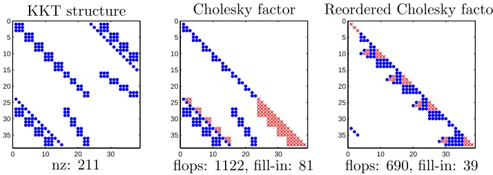
By far, the most amount of time is spent solving the linear system (3.5). However, this linear system is quite sparse for MPC problems. This allows a significant amount of pre-computation of the inverse to be made offline, see Figure 3.1 and [MWB11].
0 10 20 30
0
5
10
15
20
25
30
35
0 10 20 30
0
5
10
15
20
25
30
35
0 10 20 30
0
5
10
15
20
25
30
35
KKT structure Cholesky factor Reordered Cholesky factor
nz: 211 flops: 1122, fill-in: 81 flops: 690, fill-in: 39
Figure 3.1: Offline structure analysis for a small MPC problem (nx = 3, nu = 2, T = 4) and
a barrier method. The nonzeros of the KKT matrix are shown as circles (left). The Cholesky factor has extra fill-in nonzeros shown as crosses (middle). With the Approximate Minimum Degree (AMD) heuristic [Dav06], a reordered Cholesky factor has fewer fill-in entries (right). All these computations are performed offline, without reference to any specific MPC problem data.
3.3
Discrete-space approximate dynamic programming
3.3.1 Bounds on the value function
(mixed continuous and discrete space) found in [HR99] and the works that followed [Ran99, HR02]. This section uses notation closest to Bertsekas [BT96] to describe lower and upper bounds on the value function for discrete-space systems, and hints to why the continuous-space case is more difficult.
3.3.2 Setup
We consider a finite state Markov Decision Process. Let X = {1, . . . , n} be a finite state space andU(i)⊆ U ={1, . . . , m} the set of actions available in statei. In this formulation, the probability of transitioning from stateito statej under the controlu∈ U(i) ispij(u), with incurred stage cost g(i, u, j). Assume the transition probabilities and costs are fixed and known.
A policy is a sequenceπ ={µ0, µ1, . . .} where eachµt:X → U is a function that maps a stateito an available action in U(i). Given a policyπ, the sequence of states {i0, i1, . . .} is a Markov chain with transition probabilities
P(it+1 =j|it=i) =pij(µt(i)).
Thus, for a given policy π={µ0, µ1, . . .}, we should have n
X
j=1
pij(µt(i)) = 1, for alli= 1, . . . , n.
The expected cost of this policy when starting from an initial state iis
Vπ(i) =E
"∞ X
t=0
γtg(it, µt(it), it+1)
i0=i
#
,
whereγ ∈(0,1] is a discount factor. For the infinite horizon case, it is often convenient to consider stationary policiesπ ={µ, µ, . . .}and γ <1.
We can think of Vπ as a vector in Rn, where each component Vπ(i) corresponds to the expected cost-to-go starting at statei. The goal is to find a policy that minimizes the expected cost-to-go,
V⋆(i) = min π V
3.3.3 Bellman operator
The optimal cost-to-go satisfies the Bellman equation
V⋆(i) = min
u∈U(i)E[g(i, u, j) +γV
⋆(j)|i, u]
= min u∈U(i)
n
X
j=1
pij(u)(g(i, u, j) +γV⋆(j)), for all i= 1, . . . , n,
with the corresponding optimal policy at stept given by
µ∗t(i) = argmin u∈U(i)
E[g(i, u, j) +γV⋆(j)|i, u], for alli= 1, . . . , n.
Value iteration. For any value function vector (V(1), . . . , V(n)) define the vector TV by the Bellman operator,
(TV)(i) = min
u∈U(i)E[g(i, u, j) +γV(j)|i, u], thus the Bellman equation reads
V =TV. (3.6)
Under some regularity assumptions (e.g., [BT96]) and an infinite horizon, the Bellman equation (3.6) has a unique solutionV⋆ with a corresponding stationary policyπ∗. We can arrive at the optimal value function by value iteration,
V(k+1)=TV(k), k= 0,1, . . . .
For any starting guessV(0), the sequence{V(0), V(1), . . .}converges toV⋆.
3.3.4 Lower and upper bounds
Monotonicity. A key property of the Bellman operatorT is its monotonicity: ifV1 ≤V2, thenTV1 ≤ TV2, where the inequalities are interpreted componentwise.
Lower bound. Any functionV that satisfies the Bellman inequality
automatically satisfies V ≤ V⋆, and is a componentwise lower bound on V⋆. To see this, recursively apply T to both sides of (3.7) and use the monotonicity property,
V ≤ TV ≤ T2V ≤ · · ·=V⋆.
The Bellman inequality (3.7) defines a class of underestimators of V⋆, one of which is V⋆ itself. Members of this class capture a performance bound on the original decision problem. For example, if the transition costs are nonnegative, thenV = 0 (componentwise) is a trivial performance bound.
Upper bound. Similarly, any function that satisfies the reverse Bellman inequality
TV ≤V (3.8)
automatically satisfies V⋆ ≤V. To see this, recursively apply T to both sides of (3.8) and use the monotonicity property,
V⋆=· · · ≤ T2V ≤ TV ≤V.
Value functions that satisfy the reverse Bellman inequality (3.8) correspond to suboptimal policies, because their value is greater than or equal to the optimal value.
3.3.5 Bound optimization by linear programming
We can attempt to recoverV⋆by optimizing over the class of value function underestimators,
maximize V
subject to V ≤ TV,
(3.9)
where the variable is the value functionV, and the objective is interpreted in some scalarized way.
prob-lem (3.9) as a linear program (LP),
maximize n
X
i=1
w(i)V(i)
subject to V(i)≤ n
X
j=1
pij(u)(g(i, u, j) +γV(j)), ∀i= 1, . . . , n,∀u∈ U(i),
with variables V(1), . . . , V(n). The weights w(1), . . . , w(n) are arbitrary, as long as they are positive. The number of linear constraints isO(nm).
Similarly, we can form an LP to optimize over the class of value function overestimators by minimizing instead of maximizing, and changing the sense of the inequalities. In both cases, the optimal value functionV⋆ for the decision problem is recovered as the optimizing variable in the corresponding LP.
To make the LP useful (instead of simply solvingV =TV), we can restrict the class of underestimators by further specifying an approximating basis,
e
V(i) = N
X
k=1
αkφk(i),
where φk : X → R is a basis function, and αk is a real coefficient for all k = 1, . . . , N. Ideally, the numberN of basis functions is less than the dimensionalitynof the state space. The underapproximation LP becomes
maximize n
X
i=1 w(i)
N
X
k=1
αkφk(i)
subject to N
X
k=1
αkφk(i)≤ n
X
j=1
pij(u) g(i, u, j) +γ N
X
k=1
αkφk(j)
!
, ∀i= 1, . . . , n,∀u∈ U(i),
3.3.6 Approximation guarantees and limitations
We wish to simultaneously find functions V+ and V− in an approximating class (e.g., relative to a fixed basis) such that
V−≤V⋆≤V+,
and the difference between V+ and V− is as small as possible. To do this we might solve the LP
minimize maxi{V+(i)−V−(i)} subject to V−≤ TV−
TV+≤V+ V−, V+∈ C
(3.10)
with variables V+ and V−. Here C ⊆ Rn represents any, e.g., basis, restrictions on the approximating class. The optimal value of (3.10), say ǫ⋆, is a measure of approximation error over all states. If the overestimator and underestimator are restricted to a basis,
V+(i) = N
X
k=1
α+kφk(i), V−(i) = N
X
k=1
α−kφk(i),
then the optimization problem (3.10) has a corresponding trade-off between the number of free variables and expressiveness.
While a single-sided program like (3.9) delivers a performance bound for the decision problem, it does not relate the value function underestimate to the true value function V⋆. To relate to the true value function, we require both lower and upper bounds, since single-sided bounds can be arbitrarily poor, depending on the choice of basis. The double-sided program (3.10) gives a performance bound, a suboptimal policy, and a worst case approximation error, because the true value function is pointwise between the lower and upper estimates.
TV+≤V+. For the finite case, it holds if and only if
min u∈U(i)
n
X
j=1
pij(u)(g(i, u, j) +γV+(j))≤V+(i), ∀i= 1, . . . , n. (3.11)
In other words,V+ satisfiesTV+≤V+ if and only if for each state ithere exists an input u∈ U(i) for which the expected value is less than V+(i). The left side is not convex in the optimization variable V, because the minimum is on the wrong side of the inequality sign. This is not an issue for the Bellman inequalityV−≤ TV−, because it takes the form
V−(i)≤ min u∈U(i)
n
X
j=1
pij(u)(g(i, u, j) +γV−(j)), ∀i= 1, . . . , n,
which is suitably convex. To engineer around this difficulty, we can restrict to conditions that imply the condition (3.11). For example, the conservative condition
1 m
m
X
u=1 n
X
j=1
pij(u)(g(i, u, j) +γV+(j))≤V+(i), ∀i= 1, . . . , n,
is suitable, because an average is always at least the minimum. (This is the condition implemented to obtain the bounds of Figure 3.4.)
3.3.7 Optimization with unknown transition probabilities
If the transition probabilities pij(u) are not known ahead of time (as in an exploration or machine learning scenario), but are known to be in some set, then robust optimization can be used to design policies that are robust with respect to the uncertainty in these probabilities. As in the case of robust LP, some uncertainty descriptions are tractable.
Robust LP. Consider a linear program in inequality form,
minimize cTx subject to aT
i x≤bi, i= 1, . . . , m
over the variable x ∈Rn, where c,bi are fixed, and each ai is known to lie in an ellipsoid ai∈ Ei, where
The goal of a robust LP is to find a solution that works for all such ai ∈ Ei, which is equivalent to the optimization problem
minimize cTx
subject to supai∈Ei(aTi x)≤bi, i= 1, . . . , m.
(3.12)
Since the supremum in (3.12) is equal to
sup ai∈Ei
(aTix) =aTi x+kPiTxk2,
for everyx, we can rewrite the robust LP (3.12) as the Second Order Cone Program (SOCP)
minimize cTx subject to aT
i x+kPiTxk2≤bi, i= 1, . . . , m.
(3.13)
Notably, the problem (3.13) is convex, with efficient solution techniques for medium to large m and n. The additional terms kPiTxk2 act as norm regularization constraints.
Robust performance bound. If the transition probabilities are known to lie in an ellipsoid, then we can rewrite the robust underapproximation program
maximize n
X
i=1
w(i)V(i)
subject to V(i)≤ n
X
j=1
pij(u)(g(i, u, j) +γV(j)),
∀i= 1, . . . , n,∀u∈ U(i),∀pi:(u)∈ Ei(u),
as an SOCP. For every stateiand inputu, the outbound probability vectorpi:(u)∈ Ei(u)⊆
Rn lies an ellipsoid, andV ∈Rn is the variable. As a special case, this formulation can be used to find a value function (and policy) that is robust with respect to lower and upper bounds on the transition probabilities,
by choosing a diagonal ellipsoid that encompasses these intervals,e.g.,
Ei(u) ={ai(u) +Pi(u)v | kvk2≤1}, i= 1, . . . , n, u∈ U(i),
where
ai(u) =
pi:(u) +pi:(u)
2 , Pi(u) =
pi1(u)−pi1(u)
2 · · · 0
..
. . .. ...
0 · · · pin(u)−pin(u)
2 .
3.3.8 Example: Gridworld
We construct a state space consisting of n = 30 states, arranged in a 5×6 grid and indexed i = 1, . . . ,30 (left-right, top-bottom), modeling the movement of robot or person in a cluttered environment. At each state, there are up to four possible actionsu= 1, . . . ,4 corresponding to a movementN,W,S, andE, respectively. For each non-edge state i, the transition probability is defined as
pij(u) =
0.8 ifj neighbors i, and u is a movement toj, 0.1/3 if j neighbors i, and u is not a movement toj, 0.1 ifj=i,
0 otherwise.
Thus, for every non-edge state, there is a 0.8 chance of moving to a desired square, 0.1 chance (split evenly) to jump to one of the remaining three neighbors, and a 0.1 chance of staying at the current square. For edges and corners, we stay at the current square if a control action is unavailable.
Next, a fraction of the squares is chosen to be obstacles. These states have probability 1.0 of staying and zero probability of leaving, and are disconnected from their neighboring states.
Finally, a cost of 1 is chosen for every transition to a neighboring state, with the bottom right state (state 30) having zero cost.
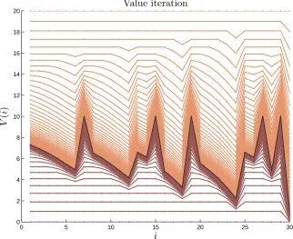
version of the optimization problem (3.10) withN = 10 basis vectors. Crucially, one of the basis vectors was a vector of the form
φobst(i) =
1 ifiis an obstacle, 0 otherwise.
To decrease basis complexity, we can use basis vectors that encode state membership constraints:
• A basis vector can pool over labeled, free, and obstacle regions.
• If a particular type of policy is expected, one can choose a basis vector whose gradient tends to point toward the goal.
0 5 10 15 20 25 30
0 2 4 6 8 10 12 14 16 18 20
i
V
(
i
)
Value iteration
Figure 3.2: Lower and upper bounds of the value function during two instances of value iteration. Here the initial guess wasV(0) = 0 for the lower bounds andV(0) = 20 for the upper bounds. Both
iterations converge in the middle.
3.4
Continuous-space approximate dynamic programming
1 2 3 4 5 6 0.5
1
1.5
2
2.5
3
3.5
4
4.5
5
5.5
2 3 4 5 6 7 8 9 10
column
ro
w
Value function after 60 iterations
Figure 3.3: Gridworld with shading indicating the cost to go after 60 value iterations. The target (bottom-right) cell has zero cost-to-go. The obstacle states areXobst=
{7,15,19,27,29}.
0 5 10 15 20 25 30
0 2 4 6 8 10 12 14 16 18 20
i
V
(
i
)
Value iteration
introduce its own level of conservativeness.
1. Continuous state space. The value function V :X →R is an infinite-dimensional object. Representing V in large dimensional states (n ≫ 1) requires exponentially many sample points to maintain adequate detail. Typically this is partially resolved by restriction to a given basis, e.g., finite elements, piecewise linear, or quadratic approximations.
2. Continuous action space. An implementation of the Bellman inequality (3.7) becomes a semi-infinite constraint indexed by the control inputu∈ U, even when the value function is finitely parameterized. Typically, S-procedure style arguments are made here.
3.4.1 Example: Linear quadratic dynamics with bounded control
The following example from [WOB14] illustrates the type of analysis required in the con-tinuous domain. Consider a discrete-time concon-tinuous space system
xt+1 =Axt+But+wt, t= 0,1, . . . ,
with initial state x0 and zero-mean noise termsw0, w1, . . . satisfying
E[wt] = 0, E[wtwtT] =W ∈Rn×n, for allt= 0,1, . . . ,
and a quadratic cost function g(x, u) = xTQx+uTRu. The state space is unbounded, X =Rn, and the controls have an upper bound,
U ={u∈Rm| kuk∞≤1}.
Note that the main difference between this problem and a standard LQR-style problem (which has a closed form solution) is the control bound. The first choice is how to represent the infinite-dimensional value function in a finite dim