Blind Component Separation in Wavelet Space: Application to CMB Analysis

(1)

Blind Component Separation in Wavelet Space:

Application to CMB Analysis

Y. Moudden

DAPNIA/SEDI-SAP, CEA/Saclay, 91191 Gif-sur-Yvette, France Email:[email protected]

J.-F. Cardoso

CNRS, École National Su´perieure des Télécommunications, 46 rue Barrault, 75634 Paris, France Email:[email protected]

J.-L. Starck

DAPNIA/SEDI-SAP, CEA/Saclay, 91191 Gif-sur-Yvette, France Email:[email protected]

J. Delabrouille

CNRS/PCC, Coll`ege de France, 11 place Marcelin Berthelot, 75231 Paris, France Email:[email protected]

Received 30 June 2004; Revised 22 November 2004

It is a recurrent issue in astronomical data analysis that observations are incomplete maps with missing patches or intentionally masked parts. In addition, many astrophysical emissions are nonstationary processes over the sky. All these effects impair data processing techniques which work in the Fourier domain. Spectral matching ICA (SMICA) is a source separation method based on spectral matching in Fourier space designed for the separation of diffuse astrophysical emissions in cosmic microwave background observations. This paper proposes an extension of SMICA to thewaveletdomain and demonstrates the effectiveness of wavelet-based statistics for dealing with gaps in the data.

Keywords and phrases:blind source separation, cosmic microwave background, wavelets, data analysis, missing data.

1. INTRODUCTION

The detection of cosmic microwave background (CMB) anisotropies on the sky has been over the past three decades a subject of intense activity in the cosmology community. The CMB, discovered in 1965 by Penzias and Wilson, is a relic ra-diation emitted some 13 billion years ago, when the universe was about 370 000 years old. Small fluctuations of this emis-sion, tracing the seeds of the primordial inhomogeneities which gave rise to present large scale structures as galaxies and clusters of galaxies, were first discovered in the observa-tions made by COBE [1] and further investigated by a num-ber of experiments among which Archeops [2], boomerang [3], maxima [4], and WMAP [5].

The precise measurement of these fluctuations is of ut-most importance to cosmology. Their statistical properties (spatial power spectrum, Gaussianity) strongly depend on the cosmological scenarios describing the properties and evolution of our universe as a whole, and thus permit to

constrain these models as well as to measure the cosmologi-cal parameters describing the matter content, the geometry, and the evolution of our universe [6].

Accessing this information, however, requires disentan-gling in the data the contributions of several distinct astro-physical sources, all of which emit radiation in the frequency range used for CMB observations [7]. This problem of com-ponent separation, in the field of CMB studies, has thus been the object of many dedicated studies in the past.

To first order, the total sky emission can be modeled as a linear superposition of a few independent processes. The observation of the sky in direction (θ,ϕ) with detectordis then a noisy linear mixture ofNccomponents:

xd(ϑ,ϕ)=

Nc

j=1

Adjsj(ϑ,ϕ) +nd(ϑ,ϕ), (1)

where sj is the emission template for the jth

(2)

The coeﬃcientsAdjreflect emission laws whilend accounts

for noise. WhenNd detectors provide independent

observa-tions, this equation can be put in vector-matrix form:

X(ϑ,ϕ)=AS(ϑ,ϕ) +N(ϑ,ϕ), (2)

whereXandNare vectors of lengthNd,Sis a vector of length

Nc, andAis theNd×Ncmixing matrix.

Given the observations of such a set of independent de-tectors, component separation consists in recovering esti-mates of the maps of the sourcessj(ϑ,ϕ). Explicit component

separation has been investigated first in CMB applications by [7,8,9]. In these applications, recovering component maps is the primary target, and all the parameters of the model (mix-ing matrixAdj, noise levels, statistics of the components,

in-cluding the spatial power spectra) are assumed to be known and are used to invert the linear system.

Recent research has addressed the case of an imperfectly known mixing matrix. It is then necessary to estimate it (or at least some of its entries) directly from the data. For in-stance, Tegmark et al. assume power law emission spectra for all components except CMB and SZ, and fit spectral indices to the observations [10].

More recently, blind source separation or independent component analysis (ICA) methods have been implemented specifically for CMB studies. The work of Baccigalupi et al. [11], further extended by Maino et al. [12], imple-ments a blind source separation method exploiting the non-Gaussianity of the sources for their separation, which permits to recover the mixing matrixAand the maps of the sources. Accounting for spatially varying instrumental noise in the observation model is investigated by Kuruoglu et al. in [13], as well as the possible inclusion of prior information about the distributions of the components using a generic Gaussian mixture model.

Snoussi et al. [14] propose a Bayesian approach in the Fourier domain assuming known spectra for the compo-nents as well as possibly non-Gaussian priors for the Fourier coeﬃcients of the components. A fully blind, maximum like-lihood approach is developed in [15,16], with the new point of view that spatial power spectra are actually the main un-known parameters of interest for CMB observations. A key benefit is that parameter estimation can then be based on a set of band-averaged spectral covariance matrices, consider-ably compressing the data size.

Working in the frequency domain oﬀers several benefits but the nonlocality of the Fourier transform creates some dif-ficulties. In particular, one may wish to avoid the averaging induced by the nonlocality of the Fourier transform when dealing with strongly nonstationary components or noise. In addition, in many experiments, only an incomplete sky cov-erage is available. Either the instrument observes only a frac-tion of the sky or some regions of the sky must be masked due to localized strong astrophysical sources of contamination: compact radio sources or galaxies, strong emitting regions in the galactic plane. These eﬀects can be mitigated in a simple manner thanks to the localization properties of wavelets.

Blind component separation (and in particular estima-tion of the mixing matrix), as discussed by Cardoso [17], can be achieved in several diﬀerent ways. The first of these ex-ploits non-Gaussianity of all, but possibly one, components. The component separation method of Baccigalupi [11] and Maino [12] belongs to this set of techniques. In CMB data analysis, however, the main component of interest (the CMB itself) has a Gaussian distribution and the observed mixtures suﬀer from additive Gaussian noise, so that better perfor-mance can be expected from methods based on Gaussian models. A second set of techniques exploits spectral diver-sity and works in the Fourier domain. It has the advantage that detector–dependent beams can be handled easily, since the convolution with a point spread function in direct space becomes a simple product in Fourier space. SMICA follows this approach in the context of noisy observations. Finally, a third set of methods exploits nonstationarity. It is adapted to situations where components are strongly nonstationary in real space.

It is natural to investigate the possible benefits of ex-ploiting both nonstationarity and spectral diversity for blind component separation using wavelets. Indeed wavelets are powerful tools in revealing the spectral content of nonsta-tionary data. Although blind source separation in the wavelet domain has been previously examined, the setting here is diﬀerent. We should mention, for instance, the separation method in [18] which is based on the non-Gaussianity of the source signals but after a sparsifyingwavelet transform and the Bayesian approach in [19] which adopts a similar point of view although with a richer source model accounting for correlations in the wavelet representation.

The paper is organized as follows. InSection 2, we first recall the principle of spectral matching ICA. Then, after a brief reminder of some properties of the `a trous wavelet transform, we discuss inSection 3the extension of SMICA to component separation in wavelet space in order to deal with nonstationary data. Considering the problem of incomplete data as a model case of practical significance for the compar-ison of SMICA and its extension wSMICA, numerical exper-iments and results are reported inSection 4.

2. SMICA

Spectral matching ICA, or SMICA for short, is a blind source separation technique which, unlike most standard ICA methods, is able to recover Gaussian sources in noisy contexts. It operates in the spectral domain and is based on

spectral diversity: it is able to separate sources provided they have diﬀerent power spectra. This section gives a brief ac-count of SMICA. More details can be found in [16]; first ap-plications to CMB analysis are in [16,20].

2.1. Model and cost function

For a second-order stationary Nd-dimensional process, we

denote byRX(ν) theNd×Ndspectral covariance matrix at

fre-quencyν, that is, the (i,i)th entry ofRX(ν) is the power

(3)

ofRX(ν) contain the cross-spectra between the entries ofX.

IfXfollows the linear model of (2) with independent addi-tive noise, then its spectral covariance matrix is structured as

RX(ν)=ARS(ν)A†+RN(ν) (3)

withRS(ν) andRN(ν) being the spectral covariance matrices

of SandN, respectively. The assumption of independence between the underlying components implies thatRS(ν) is a

diagonal matrix. We will also assume independence of the noise processes between detectors: matrixRN(ν) also is a

di-agonal matrix.

In the definition ofRX(ν), we have not explicitly defined

the frequencyν. This is because SMICA can be applied for the separation of components in many contexts: each ob-servationXdcan be a time series (one-dimensional), an

im-age (two-dimensional random fields), a random field on the sphere (as in full-sky CMB studies). In each case, the appro-priate notions of frequency, stationarity, and power spectrum should be used.

SMICA estimates all (or a subset of) the model parame-ters

θ=RS

νq

,RN

νq

,A (4)

by minimizing a measure of “spectral mismatch” between sample estimates RX(ν) (defined below) of the spectral

co-variance matrices and their ensemble averages which de-pend on the parameters according to (3). More specifically, an estimate θ = {RS(νq),RN(νq),A} is obtained as θ =

argmin_θφ(θ) where the measure of spectral mismatchφ(θ) is defined by

φ(θ)=

Q

q=1

αqDRX

νq

,ARS

νq

A†+RN

νq

. (5)

Here,{νq|1 ≤ q ≤Q}is a set of frequencies,{αq|1 ≤ q ≤

Q}is a set of positive weights, andD(·,·) is a measure of mismatch between two positive matrices.

This approach is a particular instance of moment match-ing. As such, if consistent estimatesRX(νq) of the spectral

covariance matricesRX(νq) are available and if the model is

identifiable, then any reasonable choice of the weightsαqand

of the divergence measureD(·,·) should lead toconsistent

estimates of the parameters. However, this does not mean that these choices should be arbitrary: in our standard imple-mentation, we make specific choices (described next) in such a way that minimizingφ(θ) is identical to maximizing the likelihood ofθin a model of Gaussian stationary processes. Hence, these choices guarantee a good statistical eﬃciency when the underlying processes are well modeled as Gaussian stationary processes. When this is not the case, though, the performance of SMICA may not be as good as (but not nec-essarily worse than) the performance of other methods de-signed to capture other aspects of the statistical distribution of the data, such as non-Gaussian features, for instance.

Given a data set, denote byX(ν) its discrete Fourier trans-form at frequency νand denote by{Fq|1 ≤ q ≤ Q}a set

ofQfrequency domains withFqcentered around frequency

νq. Spectral covariance matrices are estimated

nonparamet-rically by

RX

νq

= 1 nq

ν∈Fq

X(ν)X(ν)†, (6)

wherenqdenotes the number of Fourier pointsX(ν) in the

spectral domainFq. We always use symmetric domains in the

sense that frequency νbelongs toFq if and only if−νalso

does. This symmetry guarantees thatRX(νq) is always a

real-valued matrix whenXitself is a real-valued process.

In its standard form, the SMICA technique uses positive weightsαq=nqand a divergenceDdefined as

DKL

R1,R2

=1 2

traceR1R−12

−log detR1R−12

−m (7)

which is the Kullback-Leibler divergence between two m-variate zero-mean Gaussian distributions with covariance matricesR1andR2. These choices stem from the Whittle ap-proximation according to which eachX(ν) has a zero-mean normal distribution with covariance matrixRX(ν) and is

un-correlated with X(ν) for ν = ν_{. In this case, it is easily} checked that−φ(θ) evaluated withαq =nq andD =DKL is (up to a constant) the log-likelihood for Tdata samples. This is actually true when the spectral domains are shrunk to just one DFT point (nq =1 for allq); when the spectral

do-mainsFqare chosen to contain several (usually many) DFT

points, then−φ(θ) is the log-likelihood, in the Whittle ap-proximation, of the Gaussian stationary model with constant power spectrum over each domainFq. This approximation is

at small statistical loss when the spectrum is smooth enough to show little variation over each spectral domain.

The major gain of assuming constant spectrum over each Fq is the resulting reduction of the data set to a small

num-ber of covariance matrices. This may be a crucial benefit in applications like astronomical imaging where very large data sets are frequent.

Regarding our application to CMB analysis, the hypoth-esized isotropy of the distribution of the sources leads to in-tegrate over spectral domains with the corresponding sym-metry. For sky maps small enough to be considered as flat, the spectral decomposition is the two-dimensional Fourier transform and the “natural” spectral domains are rings cen-tered on the null frequency. For larger maps where curva-ture cannot be neglected, the spectral decomposition is over spherical harmonics and the natural spectral domains con-tain all the modes associated to a set of scales [20].

2.2. Parameter optimization

(4)

algorithm. This is detailed in [16] in the case of spatially white noise, that is,RN(ν) actually not depending onν.

Ac-tually, this latter algorithm was slightly modified in order to deal with the case of colored noiseN in (2). Another useful enhancement was to allow for constraints to be set on the model parameters so that prior information such as bounds on some entries of the mixing matrixAcould be included. Details are given in the appendix.

The EM algorithm is straightforwardly implemented and does not require any tuning. It can quickly drive the spec-tral mismatch down to small values but is often unable to complete the optimization. Slow EM finishing is inherent to noisy models [21] and we have found it necessary to imple-ment a mixedad hocstrategy based on alternating EM steps and BFGS steps [16].

We have also found that initialization is critical: criterion (5) is probably multimodal for many data sets. This issue is not addressed in this paper though, since our prime inter-est is in the study of the statistical performances of diﬀerent estimators of the model parametersθ. In the simulations re-ported below, the minimization of φ(θ) is initialized at the true mixing matrix and with spectral covariance matrices es-timated from the initial separate source and noise maps.

2.3. Component map estimation

When running SMICA, power spectral densities for the sources and detector noise are obtained along with the es-timated mixing matrix. They are used in reconstructing the source mapsviaWiener filtering in Fourier space: a Fourier modeX(ν) in frequency bandν∈Fqis used to reconstruct

the maps according to

S(ν)=A†RN(ν)−1A+RS(ν)−1 −1

A†RN(ν)−1X(ν). (8)

In the limiting case where noise is small compared to signal components, the Wiener filter reduces to

S(ν)=A†RN(ν)−1A −1

A†RN(ν)−1X(ν). (9)

Note however that the above Wiener filter is optimal only in front of stationary Gaussian processes. For weak, point-like sources such as galaxy clusters seen via the Sunyaev– Zel’dovich eﬀect (defined inSection 4.1), much better recon-struction can be expected from nonlinear methods.

3. SPECTRAL MATCHING IN WAVELET SPACE

The SMICA method for spectral matching in Fourier space has already shown significant success for CMB spectral esti-mation in multidetector experiments. It is in particular able to identify and remove residuals of poorly known correlated systematics and astrophysical foreground emissions contam-inating CMB maps. However, SMICA suﬀers from several practical diﬃculties when dealing with real data.

Indeed, actual components are known to depart slightly from the ideal linear mixture model (2). The mixing matrix

(in particular those columns ofAwhich correspond to galac-tic emissions) is known to depend somewhat on the direction of observation or on spatial frequency. Measuring the depen-denceA(ϑ,ϕ) is of interest for future experiments as Planck, and cannot be achieved directly with SMICA. Further, the components are known to be both correlated and nonsta-tionary. For instance, galactic dust emissions are strongly peaked towards the galactic plane. A nonlocal spectral repre-sentation (viaFourier coeﬃcients orviaspherical harmon-ics) mixes contributions from high galactic sky, nearly free of foreground contamination, and contributions from within the galactic plane. Noise levels themselves may be quite non-stationary, with high SNR regions observed for a long time and low SNR regions poorly observed.

When there are sharp edges on the maps or gaps in the data, corresponding to unobserved or masked regions, spec-tral estimation using the smooth periodogram of (6) is not the most satisfactory procedure. Although apodizing win-dows may help cope with edge eﬀects in Fourier analysis, they are not very straightforward to use in the case of arbitrarily shaped maps with arbitrarily shaped gaps, such as those en-countered in the Archeops experiment [2].

Clearly, the spectral analysis of gapped data requires tools diﬀerent from those used to process full data sets, if only be-cause the hypothesized stationarity of the data is greatly dis-turbed by the missing samples. Common such methods of-ten amount to using standard spectral estimators after the gaps were filled with estimates of the missing samples. How-ever, the data interpolation stage is critical and cannot be completed without prior assumptions on the data. Another idea, applicable to CMB analysis, is to process gapped data as if they were complete but to correct afterwards the spec-tral estimates from the bias induced by the gaps [22]. We preferred to rely on methods intrinsically dedicated to the analysis of nonstationary data such as the wavelet transform, widely used to reveal variations in the spectral content of time series or images, as they permit to single out regions in direct space while retaining localization in the frequency domain. We see next how to reformulate (5) in the wavelet domain in order to deal with missing data. Note that, in the following, the locations of the missing samples are assumed to be known.

3.1. Wavelet transform

(5)

which contain only isotropic features. The undecimated isotropic à trouswavelet transform has been shown to be well suited to the analysis of astrophysical data where transla-tion invariance is desirable and where the emphasis is seldom on data compression [23]. Further, with this choice of scal-ing function, the so-called scalscal-ing equation is satisfied, and therefore fast implementations of the decomposition and re-construction steps of theà troustransform are available [23]. Given a 2D data setc0(k,l), the à trousalgorithm pro-duces recursively a set of detail mapswi(k,l) on a dyadic

res-olution scale and a smooth approximationcJ(k,l) [23]. We

note that the lowest resolution Jmax is obviously limited by the data map size. The transform is readily inverted by

c0(k,l)=cJ(k,l) + J

i=1

wi(k,l), (10)

which is a simple addition of the smooth array with the detail maps.

3.2. Spectral matching in wavelet space: wSMICA In order to define a sensible wavelet version of SMICA, we first rewrite the SMICA criterion (5) in terms of covariance matrices in the initial domain, where, for instance, the gaps are best described, rather than in the Fourier domain.

Consider a batch ofT data samplesXt=1,T wheretis an

appropriate index depending on the dimension of the data, and the set ofQideal bandpass filtersFqassociated with the nonoverlapping frequency domainsFqused in SMICA.

De-noting byXq(t) the data filtered throughFq, we define

sam-ple covariance matrices

RT,X(q)= 1

T

t=1

Xq(t)Xq(t)† (11)

obtained by averaging in the original domain. Owing to the unitary property of the discrete Fourier transform, one has

RT,X(q)= nq

TRX

νq

, (12)

where nq was defined as the number of Fourier modes in

spectral bandFq. These matrices are estimates ofRT,X(q)=

E(Xq(t)Xq(t)†), the covariance matrix ofXq(t). Again,

ac-cording to model (3), the covariance matrices are again structured as

RT,X(q)=ART,S(q)A†+RT,N(q), (13)

whereRT,S(q) andRT,N(q) are defined similarly toRT,X(q).

Hence, minimizing the SMICA objective function (5) is then equivalent to minimizing

φ(θ)=

Q

q=1

nqDKL

RT,X(q), ART,S(q)A†+RT,N(q)

(14)

with respect to the new set of parametersθ = (A,RT,S(q),

RT,N(q)).

0 0.05 0.1 0.15 0.2 0.25 0.3 10−16

10−14 10−12 10−10 10−8 10−6 10−4 10−2 100

Reduced frequency

M

ag

nitude

Figure 1: Magnitudes averaged over spectral rings of the nearly isotropic cubic spline wavelet filtersψ1,ψ2,. . .,ψ5used in the

sim-ulations described further down. The vertical dotted lines forν= {0.013, 0.025, 0.045, 0.09, 0.2}delimit the five frequency bands used with SMICA in these simulations.

We now consider using another set of filters in place of the ideal bandpass filters used by SMICA. In dealing with nonstationary data or, as a special case, with gapped data, it is especially attractive to consider finite impulse response (FIR) filters. Indeed, provided the response of such a filter is short enough compared to data sizeTand gap widths, most of the samples in the filtered signal will be unaﬀected by the presence of gaps. Using exclusively these samples yields esti-mated covariance matrices which are not biased by the miss-ing data, at the cost of a slight increase of variance due to discarding some data samples. In the following, we use fil-ters ψ1,ψ2,. . .,ψJ,φJ (seeFigure 1) and the wavelet`a trous

algorithm.

Consider again a batch ofTregularly spaced data samples Xt=1,T. Possible gaps in the data are simply described with a

maskµ, that is, an array of zeroes and ones of the same size as the dataXt=1,T with ones corresponding to samples outside

the gaps. Denoting by W1,W2,. . .,WJ andCJ the wavelet

scales and the smooth approximation of X, obtained with the`a troustransform andµ1,. . .,µJ+1the masks for the dif-ferent scales determined from the original maskµknowing the diﬀerent filter lengths, wavelet covariances are estimated as follows:

RW,X(1≤i≤J)=

1 li

T

t=1µi

(t)Wi(t)Wi(t)†,

RW,X(J+ 1)= 1

lJ+1 T

t=1

µJ+1(t)CJ(t)CJ(t)†,

(15)

whereliis the number of nonzero samples inµi. With source

and noise covariances RW,S(i),RW,N(i) defined in a similar

way, the covariance model in wavelet space becomes

(6)

(a) (b) (c)

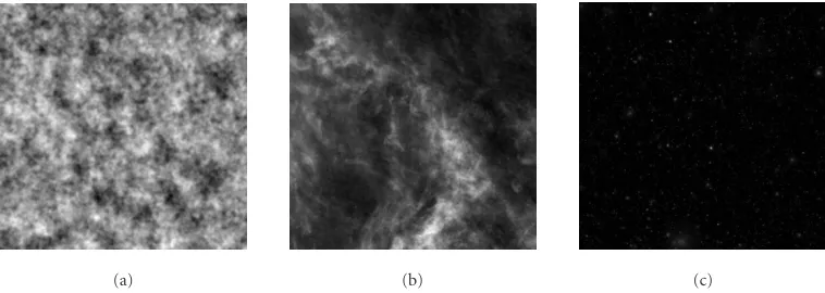
Figure2: Samples of simulated component maps of CMB, dust, and SZ.

Our wavelet-based version of SMICA consists in minimizing the wSMICA criterion:

φ(θ)=

J+1

i=1

αiDKL

RW,X(i),ARW,S(i)A†+RW,N(i)

(17)

with respect to θ = (A,RW,S(i),RW,N(i)) for some sensible

choice of the weightsαi.

The weights in the spectral mismatch (17) should be cho-sen to reflect the variability of the estimate of the correspond-ing covariance matrix. Examincorrespond-ing first (14), we see weights which are proportional tonq, that is, to the number of DFT

points used in computing the sample covariance matrix, be-cause this is in fact the number of uncorrelated values ofX(ν) entering in the estimation ofRX(νq). It is also proportional to

the size of the frequency domain over whichRX(νq) is

eval-uated. Since wSMICA uses wavelet filters with only limited overlap, we choose to use the same strategy as in SMICA since the latter amounts to using ideal bandpass filters. In other words, when no data points are missing, the weights for wSMICA are taken proportional to the size of the frequency domains covered at each scale. This is

α1,α2,. . .,αJ,αJ+1

=

1 2,

1 4,. . .,

1 2J,

1 2J

(18)

in the one-dimensional case and

α1,α2,. . .,αJ,αJ+1

=

3 4,

3 16,. . .,

3 4J,

1 4J

(19)

in the two-dimensional case.

In the case of data with gaps, we must further take into account that some wavelet coeﬃcients are discarded. Letβi

denote the fraction of wavelets coeﬃcients which are unaf-fected by the gaps at scalei. The number of eﬀective points is reduced by this fraction and one should use the weights

α1,α2,. . .,αJ,αJ+1

=

β1 2,

β2 4,. . .,

βJ

2J,

βJ+1 2J

(20)

in the one-dimensional case and

α1,α2,. . .,αJ,αJ+1

=

3β1 4 ,

3β2 16,. . .,

3βJ

4J ,

βJ+1 4J

(21)

in the two-dimensional case. The fraction 1−βiof discarded

points depends on scalei(even with the`a trousalgorithm) because the length of the wavelet filter itself depends on i. However, it is roughly scale independent, if the missing data are large patches of much bigger size than the length of the wavelet filters used at any scale in the wavelet decomposition. Before closing, we note that the diﬀerent wavelet filter outputsWi(t) are correlated due to the overlap between

fre-quency responses (Figure 1). Optimal inference should take this correlation into account but we have chosen not to do so and rather to stick to a simple criterion like (17) which ig-nores the correlations between sample covariance matrices. No big loss is expected from this choice because the wavelet bands do not overlap very much.

4. NUMERICAL EXPERIMENTS

4.1. Simulation of realistic maps

We have simulated observations consisting of m = 6 mix-tures ofn=3 components, namely, CMB, galactic dust, and SZ emissions for which templates were obtained as described in [16]; seeFigure 2for typical realizations.

Dust emission is the greybody emission of small dust particles in our own galaxy. The intensity of emission is strongly concentrated towards the galactic plane, although cirrus clouds at high galactic latitudes are present as well. The dust emission law is of the formνα_Bν_(T

dust) whereα1.7, Bν(T) is the blackbody emission law, andTdust17 K is the typical dust temperature in the interstellar medium.

(7)

(a) (b) (c)

(d) (e) (f)

Figure3: Simulated observation maps based on the templates shown inFigure 2and the mixing matrix inTable 1for the nominal Planck HFI noise levels.

Table1: Entries ofA, the mixing matrix used in our simulations.

CMB Dust SZ Channel

7.452×10−1 3.654×10−2 −8.733×10−1 100 GHz

5.799×10−1 ₇_.₀₂₁_×₁₀−2 ₋₄_.₆₈₉_×₁₀−1 _{143 GHz}

3.206×10−1 1.449×10−1 −2.093×10−3 217 GHz

7.435×10−2 3.106×10−1 1.294×10−1 353 GHz

6.009×10−3 ₅_.₃₉₈_×₁₀−1 ₂_.₆₁₃_×₁₀−2 _{545 GHz}

6.115×10−5 ₇_.₆₄₈_×₁₀−1 ₅_.₂₆₈_×₁₀−4 _{857 GHz}

energy distribution, depleting the occupation of low energy levels and populating high energy levels. The net eﬀect, to first order, is a small additive emission, negative at frequen-cies below 217 GHz, and positive at frequenfrequen-cies above. A re-view on SZ eﬀect can be found in [24].

The templates, and thus the mixtures in each simulated data set, consist of 300×300 pixel maps corresponding to a 12.5◦×12.5◦ field located at high galactic latitude. The six mixtures in each set mimic observations that will eventually be acquired in the six frequency channels of the Planck HFI (Figure 3). The entries of the mixing matrixAused in these simulations actually are estimated values of the electromag-netic emission laws of each component at 100, 143, 217, 353, 545, and 857 GHz; seeTable 1.

White Gaussian noise is added to the mixtures accord-ing to model (2) in order to simulate instrumental noise.

While the relative noise standard deviations between chan-nels are set according to the nominal values of the Planck HFI, we also experiment with fiveglobalnoise levels at−20, −6,−3, 0, and +3 dB from nominal values.Table 2gives the typical energy fractions that are contributed by each of the n=3 original sources and noise, to the total energy of each of them=6 mixtures, considering Planck nominal noise vari-ance. In fact, because SMICA and wSMICA actually work on spectral bands, a much better indication of signal-to-noise ratio in these simulations is given byFigure 4which shows how noise and source energy contributions distribute with respect to frequency in the six mixtures.

(8)

Table2: Energy fraction contributed by each source to the total energy of each mixture, for the nominal noise variance on the Planck HFI channels.

CMB Dust SZ Noise Channel

9.91×10−1 1.18×10−4 7.92×10−3 2.53×10−6 100 GHz

9.97×10−1 7.25×10−4 3.79×10−3 5.17×10−7 143 GHz

9.98×10−1 ₁_.₀₁_×₁₀−2 ₂_.₄₈_×₁₀−7 ₁_.₃₄_×₁₀−7 _{217 GHz}

5.55×10−1 ₄_.₈_×₁₀−1 ₉_.₇₈_×₁₀−3 ₇_.₄₇_×₁₀−8 _{353 GHz}

2.5×10−3 1.0 2.75×10−4 3.78×10−9 545 GHz

1.29×10−7 ₁_.₀ ₅_.₅₆_×₁₀−8 ₁_.₂₄_×₁₀−10 _{857 GHz}

was also considered as a reference case. Spectral matching with wSMICA is conducted using the output of the five wavelet filters ψ1,. . .,ψ5 associated to higher frequency de-tails. For the sake of comparison, SMICA is run using five bands in Fourier space which are similar to the dyadic bands imposed by the wavelet transform, as shown inFigure 1. This latter choice of frequency bands is made to ease comparison between SMICA and wSMICA.

4.2. Experiments with noise-free mixtures

Preliminary experiments were conducted in the case of van-ishing instrumental noise variance. In this case, the blind component separation problem is “equivariant,” entailing that the quality of separation on a given mixture does not depend at all on the mixing matrix Abut only on the par-ticular realization of the sources and on the algorithm used for separation. More specifically, in the case of SMICA and wSMICA, separation performance depends on the spectral diversity of the components and on the ability of both objec-tive functions to exploit this diversity. Hence, the noise-free experiments in this section are indicative of the spectral di-versity of the components, of the ability of (w)SMICA to cap-ture it, and of the robustness of the (w)SMICA with respect to missing data.

Note that in a noise-free model, the spectral matching objective boils down to an objective of joint diagonalization of the covariance matrices, as shown in [25]. Hence, spectral matching can be implemented using an eﬃcient dedicated algorithm [26].

The estimated components are related to the true one ac-cording to

S=IS, (22)

whereIis the product of the mixing matrix used in simula-tions and of the separating matrix obtained by joint diago-nalization. It also includes any normalization needed for the components and their estimates to have total energy in all bands equal to 1. With this normalization, the square of any oﬀdiagonal termIi j is directly related to the residual level of contamination by component jin the recovered compo-nenti. Since performance in separating noise-free mixtures is independent of the mixing matrix, the choice ofAin the simulations is irrelevant: it does not change the distribution ofI. In practice, our noise-free experiments are conducted

without any mixing, that is, we takeAto be the 3×3 identity matrix. The following steps were repeated 1000 times.

(i) Randomly pick one of each component maps out of the available 200 CMB maps, 30 dust maps, and 1500 SZ maps.

(ii) Compute covariance matrices in the five wavelet or Fourier bands, both with and without masking part of the maps.

(iii) Normalize each source so that its total energy over the five bands is equal to one.

(iv) Estimate a separating matrix by joint diagonalization of the covariance matrices.

These noise-free experiments are complemented using “surrogate” data in order to assess the eﬀect of any non-Gaussianity or nonstationarity in the source templates. We repeat the simulations on Gaussian stationary maps gener-ated with the same spectra as the CMB, dust, and SZ compo-nents. The resulting distribution ofIthen only reflects the ability of (w)SMICA to exploit the spectral diversity of the components independently of the other aspects of their dis-tribution.

The histograms onFigure 6are for the oﬀdiagonal term corresponding to the residual corruption of CMB by Gaus-siandust in the second set of experiments (using surrogate data). In Tables 3and4, the results obtained with the syn-thetic component maps are given as well as those obtained with the surrogate Gaussian maps, in terms of the standard deviations of the oﬀdiagonal entriesIi jdefined by (22).

(9)

0 0.05 0.1 0.15 0.2 0.25 0.3 10−9

10−8 10−7 10−6 10−5 10−4 10−3 10−2 10−1 100

Reduced frequency

Energ

y

Dust

Noise CMB

SZ

(a)

0 0.05 0.1 0.15 0.2 0.25 0.3 10−8

10−7 10−6 10−5 10−4 10−3 10−2 10−1 100

Reduced frequency

Energ

y

Dust

Noise CMB

SZ

(b)

0 0.05 0.1 0.15 0.2 0.25 0.3 10−12

10−10 10−8 10−6 10−4 10−2 100

Reduced frequency

Energ

y

Dust Noise CMB

SZ

(c)

0 0.05 0.1 0.15 0.2 0.25 0.3 10−8

10−7 10−6 10−5 10−4 10−3 10−2 10−1

Reduced frequency

Energ

y

Dust

Noise CMB

SZ

(d)

0 0.05 0.1 0.15 0.2 0.25 0.3 10−10

10−9 10−8 10−7 10−6 10−5 10−4 10−3 10−2 10−1

Reduced frequency

Energ

y

Dust

Noise CMB

SZ

(e)

0 0.05 0.1 0.15 0.2 0.25 0.3 10−14

10−12 10−10 10−8 10−6 10−4 10−2 100

Reduced frequency

Energ

y

Dust

Noise

CMB

SZ

(f)

Figure4: Energy contributed by each source and noise in each bolometer as a function of frequency, for the nominal noise variance on the Planck HFI channels: (a) 100 GHz, (b) 143 GHz, (c) 217 GHz, (d) 353 GHz, (e) 545 GHz, and (f) 857 GHz. Note how SZ is expected to be always below nominal noise, that CMB and dust strongly dominate in diﬀerent channels, and that CMB and dust spectra, without being proportional, display the same general behavior dominated by low modes.

spectra are somewhat similar, that is, show low spectral di-versity, and further smoothing can only degrade the perfor-mance of the source separation algorithm based on Fourier covariances.

(10)

(a) (b)

(c) (d)

(e) (f)

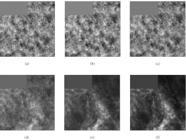
Figure5: (a) Mask used to simulate a gap in the data. (b)–(f) Mod-ified masks at scales 1 through 5. The discarded pixels are in black.

the case with covariances in Fourier space. Next, whether covariance matrices are computed in Fourier space or in wavelet space, we note that the terms coupling CMB and dust are again much higher than with surrogate data, even on complete maps. This is probably to be attributed to the nonstationarity and/or non-Gaussianity of the Dust com-ponent. Another point is that the CMB and dust templates as inFigure 2exhibit sharp edges compared to SZ and this inevitably disturbs spectral estimation using a simple DFT. To assess this eﬀect, simulations were also conducted where the covariances in Fourier space were computed after an apodizing Hanning window was applied on the complete data maps. The results reported inTable 3, to be compared toTable 4, do indicate a slightly positive eﬀect of windowing, but still the separation using wavelet-based statistics appears better. To further complete this preliminary study, we con-ducted similar experiments using JADE [27], an ICA algo-rithm based on fourth-order statistics. This algoalgo-rithm does not use spectral information at all. As discussed earlier, such a method is not expected to work well on CMB data and the results reported in Table 5do show lower performance in comparison to Tables3and4.

4.3. Realistic experiments

The results of the previous section show that, in the noise-less case, using wavelet-based covariance matrices provides a simple and eﬃcient way to cancel the bad impact that gaps actually have on the performance of estimation using Fourier-based statistics. We move on to investigate the eﬀect of additive noise on SMICA and wSMICA.

Picking at random one of each component maps out of the available 200 CMB maps, 30 dust maps, and 1500 SZ maps, 1000 sets of six synthetic mixture maps were gener-ated as previously described, for each of the 5 noise levels chosen. Then, component separation was conducted using the spectral matching algorithms SMICA and wSMICA both with and without part of the maps being masked. A typi-cal run of SMICA or wSMICA in the setting considered here (i.e., 300 by 300 maps, 6 mixtures, 3 sources, 5 wavelet scales, no constraints on the mixing matrix) takes only a few sec-onds on a 1.25 Ghz Mac G4 when coded in IDL. The same optimization techniques are used for SMICA and wSMICA since the two criteria have the same form.

Each run of SMICA and wSMICA on the data returns es-timatesAf andAwof the mixing matrix. These estimates are

subject to the indeterminacies inherent to the instantaneous linear mixture model (2). Indeed, in the case where optimiza-tion is over all parametersθ, any simultaneous permutation of the columns of Aand of the lines ofSleaves the model unchanged. The same occurs when exchanging a scalar pos-sibly negative factor between any column inAand the corre-sponding line inS. Therefore, columnwise comparison ofAf

andAw to the original mixing matrixArequires first fixing

these indeterminacies. This is done “by hand” afterAf and

Awhave been normalized columnwise.

The results we report next focus on the statistical proper-ties ofAf andAwas estimated from the 1000 runs of the two

competing methods in the several configurations retained. In fact, the correct estimation of the mixing matrix in model (2) is a relevant issue, for instance, when it comes to deal-ing with the cross-calibration of the diﬀerent detectors. Fig-ures7,8, and9show the results obtained, using the quadratic norm

QEj=

_m

i=1

Ai j−Ai j 21/2

(23)

withA=Af orAwandj=CMB, dust, or SZ, to assess the

residual errors on the estimated emissivities of each compo-nent. The plotted curves show how the mean of the above positive error measure varies with increasing noise variance. For the particular case of CMB, Table 6gives the estimated standard deviations of the relative errors (Ai j−Ai j)/Ai jon the

estimated CMB emission law in the six channels of Planck’s HFI in the diﬀerent configurations retained.

Closer to our source separation objective, a more signif-icant way of assessing the quality ofAf andAw as

(11)

−0.1 −0.05 0

P

rop

or

ti

on

of

co

unts

0.05 0.1 0

0.05 0.1 0.15 0.2 0.25

Oﬀdiagonal entry (a)

−0.1 −0.05

P

rop

or

ti

on

of

co

unts

0 0.05 0.1 0

0.05 0.1 0.15 0.2 0.25

Oﬀdiagonal entry (b)

Figure6: Histograms of the oﬀdiagonal term ofI, defined in (22), corresponding to the residual corruption of “CMB” by “dust” while separating Gaussian maps generated with the same power spectra as the astrophysical components, by joint diagonalization of covariance matrices in (a) Fourier and (b) wavelet spaces, with(black, which appears grey when seen through white )and without(white)masking part of the data. The dark widest histogram on the left highlights the impact of masking on source separation based on Fourier covariance matrices.

Table3: Standard deviations of the oﬀdiagonal entriesIi jdefined by (22) obtained while separating realistic component maps by joint

diagonalization of covariance matrices inFourierspace, with (M) or without masking (NM) part of the data, or applying an apodizing Hanning window (Han). Components 1, 2, and 3, respectively, stand for CMB, dust, and SZ. The numbers initalicwere obtained with Gaussian maps and the underlined numbers correspond to the histograms inFigure 6.

Oﬀdiag. entry NM M Han

I1,2 0.097 0.0076 0.074 0.038 0.024

I1,3 0.0049 0.0044 0.005 0.006 0.0094

I2,1 0.017 0.0066 0.018 0.01 0.017

I2,3 0.0064 0.0077 0.0066 0.0096 0.011

I3,1 0.0024 0.0026 0.0028 0.0037 0.0039

I3,2 0.0054 0.0071 0.0054 0.0079 0.01

Table4: Standard deviations of the oﬀdiagonal entriesIi jdefined by (22) obtained while separating realistic component maps by joint

diagonalization of covariance matrices inwaveletspace, with (M) and without masking (NM) part of the data. Components 1, 2, and 3, respectively, stand for CMB, dust, and SZ. The numbers initalicwere obtained with Gaussian maps and the underlined numbers correspond to the histograms inFigure 6.

Oﬀdiag. entry NM M

I1,2 0.015 0.0071 0.018 0.0079

I1,3 0.0025 0.0029 0.0028 0.0031

I2,1 0.016 0.0077 0.019 0.0089

I2,3 0.0041 0.0051 0.0048 0.0075

I3,1 0.0024 0.0029 0.003 0.0039

(12)

Table5: Standard deviations of the oﬀdiagonal entriesIi jdefined

by (22) obtained while separating realistic component maps using JADE, with (M) and without masking (NM) part of the data. Com-ponents 1, 2, and 3, respectively, stand for CMB, dust, and SZ.

Oﬀdiag. entry I1,2 I1,3 I2,1 I2,3 I3,1 I3,2

NM 0.021 0.25 0.022 0.02 0.31 0.02 M 0.023 0.29 0.025 0.018 0.34 0.018

interference-to-signal ratio:

ISRj=

i=jI2j,iσi2

I2

j,jσ2j

, (24)

where theσjare the source variances and

I=A†R−1N A −1

A†R−1N A (25)

withRN the noise covariance. The plots on Figures 10,11,

and12show how the mean ISR from the 1000 runs of SMICA and wSMICA in diﬀerent configurations varies with increas-ing noise.Figure 13typically estimated component maps ob-tained using SMICA and wSMICA. For the sake of compari-son, component maps estimated using the JADE source sep-aration method are also included.

We note again that the performance of wSMICA behaves as expected when noise increases and if part of the data is missing. However, this is not always the case with SMICA. Finally, this set of simulations, conducted in a more realistic setting with respect to ESA’s Planck mission, again confirms the higher performance, over Fourier analysis, that we indeed expected from the use of wavelets. The latter are able to cor-rectly grab the spectral content of partly masked data maps and from there allow for better component separation.

5. CONCLUSION

This paper has presented an extension of the spectral match-ing ICA algorithm to the wavelet domain, motivated by the need to deal with components which exhibit spatial correlations and are nonstationary. Maps with gaps are a particular instance of practical significance. Substituting co-variance matching in Fourier space by coco-variance matching in wavelet space makes it possible to cope with gaps of any shape in a very straightforward manner. Mainly, it is the finite length of the wavelet filters used here that allows the impact of edges and gaps on the estimated covariances and hence on component separation to be lowered. Optimally choosing the FIR filter bank regarding a particular application is a possible further enhancement.

Our numerical experiments, based on realistic simula-tions of the astrophysical data expected from the Planck mis-sion, confirm the benefits of correctly processing existing gaps. Clearly, other possible types of nonstationarities in the collected data such as spatially varying noise or component variance, and so forth could be dealt with very simply in a similar fashion using the wavelet extension of SMICA.

Regarding future work, a few points are in order. First, we note that possible correlations between the components are not accounted for in SMICA or wSMICA as presented here. However, it is not diﬃcult in principle to handle such known or suspected correlations by adding oﬀdiagonal pa-rameters in the model spectral covariances of the sources. Still, in the case of CMB analysis from high frequency obser-vations which contain only one galactic component (dust) as in our simulations, spatial correlations between components should not be a problem.

We note that the proposed wavelet-based approach, as implemented with the standard à trouswavelet transform, offers little flexibility in the spectral bands available for wS-MICA while the Fourier approach gives complete flexibility in this respect. But it is possible, even straightforward, to use other transforms such as the à trous wavelet packet trans-form, or thecontinuouswavelet transform, or in fact any set of linear filters, preferably FIR filters. This in turn raises the question of optimally choosing this set of filters, keeping in mind that higher resolution in Fourier space requires longer filters, which is not desirable in the case of incomplete or nonstationary data. In fact, the optimal selection of bands is clearly a meaningful question both for SMICA and wSMICA. We also note that in the CMB application, the com-ponents have quite different statistical properties: some are expected to be very close to Gaussian (like the CMB) whereas others are strongly non-Gaussian (like SZ). The non-Gaussianity of some components does not affect the consistency of our estimator but, for a given spectrum, it does affect the distribution of the estimates although this im-pact is not easily predicted. It is clear, however, that ignoring the strong non-Gaussianity of some components is a loss of information. Devising a method able, with reasonable com-plexity, to exploit jointly non-Gaussianity (as in traditional ICA techniques) and spectral information (as in Fourier or wavelet SMICA) appears as a difficult challenge.

APPENDIX

EM ALGORITHM WITH CONSTRAINTS ON THE MIXING MATRIX

Considering Q separate frequency bands of size nq with

nq = 1, the EM functional derived for the

instanta-neous mixing model (2) with independent Gaussian station-ary sourcesSand noiseNis

Φ(θ,θ)=ElogpX,S|θ|θ (A.1)

with θ = (A,RS,1,. . .,RS,Q,RN,1,. . .,RN,Q) and θ = (A,

RS,1,. . .,RS,Q,RN,1,. . .,RN,Q). The maximization step of the

(13)

−20 −6 −3 0 3 0.003

0.004 0.005 0.006 0.008

Noise level in dB relative to nominal values

Me

an

sq

u

ar

ed

er

ro

r

Fourier + Hanning Fourier + mask Fourier + no mask

Wavelet + no mask Wavelet + mask

Figure7: Comparison of the mean squared errors on the estima-tion of the emission law of CMB as a funcestima-tion of noise in five dif-ferent configurations: wSMICA without mask, wSMICA with mask, fSMICA without mask, and fSMICA with mask, and fSMICA with Hanning apodizing window.

−20 −6 −3 0 3

0.05 0.1 0.2 0.3 0.4

Me

an

sq

u

ar

ed

er

ro

r

Figure8: Comparison of the mean squared errors on the estima-tion of the emission law ofdustas a function of noise in five diﬀ er-ent configurations: wSMICA without mask, wSMICA with mask, fSMICA without mask, and fSMICA with mask, and fSMICA with Hanning apodizing window.

Linear equality constraints

WhenAis subject to linear constraints, the joint maximiza-tion of the EM funcmaximiza-tional with respect to all model parame-ters is no longer easily achieved in general. In fact, one cannot simply decouple the reestimating rules for the noise param-eters and the mixing matrix and these have to be optimized separately. We give next the modified reestimating equations for the mixing matrix and the source variances in the case of constant noise (i.e.,θ=(A,RS,1,. . .,RS,Q)).

−20 −6 −3 0 3

10−2 10−1

Me

an

sq

u

ar

ed

er

ro

r

Figure9: Comparison of the mean squared errors on the estima-tion of the emission law of SZ as a funcestima-tion of noise in five diﬀerent configurations: wSMICA without mask, wSMICA with mask, fS-MICA without mask, fSfS-MICA with mask, and fSfS-MICA with Han-ning apodizing window.

First, we exhibit the quadratic dependence of the EM functionalΦ(θ,θ) onA:

Φ(θ,θ)

= −1 2

q

nqtrace

ARss

qA†R−1N,q−ARxsq†R−1N,q−RxsqA†R−1N,q

+ constA,

(A.2)

where

Cq=

A†R−1N,qA+R−1S,q −1

,

Wq=

A†R−1N,qA+R−1S,q −1

A†R−1N,q,

Rxs

q =RX,qWq†,

Rss

q =WqRX,qWq†+Cq.

(A.3)

In the white noise case,RN,q=RN, (A.2) becomes

Φ(θ,θ)= −1 2trace

A−Rxs_Rss−1_Rss_A₋_Rxs_Rss−1† R−1N

+ constA,

(A.4)

where

Rxs=

q

nqRxsq, Rss=

q

nqRssq. (A.5)

Again, this can be rewritten as

Φ(θ,θ)= −1

2(A−M)

†_Q₍_A₋_M_{) + const}

(14)

Table6:Standard deviationsof the relative errors on the estimated emission lawsAi1of CMB in Planck’s HFI six channels. The column

labels WNM, WM, FNM, FM, FHan are for the diﬀerent configurations, respectively: wSMICA without mask, wSMICA with mask, fSMICA without mask, fSMICA with mask, and fSMICA with Hanning apodizing window. The five figures in each box are for noise variance -20, -6, -3, 0, and 3 dB from nominal Planck values.

Emission law WNM WM FNM FM FHan

4.4∗10−4 5.0∗10−4 6.2∗10−4 7.3∗10−4 7.2∗10−4

5.4∗10−4 ₇_.₅_∗₁₀−4 ₇_.₁_∗₁₀−4 ₈_.₅_∗₁₀−4 ₉_.₅_∗₁₀−4

A11 6.6∗10−4 9.2∗10−4 8.2∗10−4 8.9∗10−4 1.3∗10−3

9.4∗10−4 1.2∗10−3 1.0∗10−3 1.0∗10−3 1.7∗10−3

1.2∗10−3 ₁_.₇_∗₁₀−3 ₁_.₂_∗₁₀−3 ₁_.₄_∗₁₀−3 ₂_.₃_∗₁₀−3

1.6∗10−4 2.1∗10−4 2.1∗10−4 2.0∗10−4 2.7∗10−4

5.3∗10−4 7.8∗10−4 5.6∗10−4 5.7∗10−4 1.0∗10−3

A21 7.0∗10−4 1.1∗10−3 7.6∗10−4 8.4∗10−4 1.4∗10−3

1.0∗10−3 1.6∗10−3 1.0∗10−3 1.0∗10−3 2.1∗10−3

1.4∗10−3 2.2∗10−3 1.5∗10−3 1.7∗10−3 3.1∗10−3

1.5∗10−3 ₁_.₈_∗₁₀−3 ₂_.₂_∗₁₀−3 ₂_.₅_∗₁₀−3 ₂_.₃_∗₁₀−3

1.7∗10−3 2.1∗10−3 2.3∗10−3 2.6∗10−3 2.9∗10−3

A31 2.1∗10−3 2.6∗10−3 2.6∗10−3 2.8∗10−3 3.7∗10−3

2.7∗10−3 ₃_.₀_∗₁₀−3 ₂_.₉_∗₁₀−3 ₃_.₀_∗₁₀−3 ₄_.₂_∗₁₀−3

3.3∗10−3 4.6∗10−3 3.3∗10−3 3.5∗10−3 6.1∗10−3

1.8∗10−2 2.0∗10−2 2.7∗10−2 3.0∗10−2 2.5∗10−2

1.9∗10−2 ₂_.₁_∗₁₀−2 ₂_.₇_∗₁₀−2 ₂_.₁_∗₁₀−2 ₂_.₇_∗₁₀−2

A41 2.1∗10−2 2.4∗10−2 2.8∗10−2 3.1∗10−2 2.9∗10−2

2.7∗10−2 2.8∗10−2 3.1∗10−2 3.0∗10−2 3.5∗10−2

3.0∗10−2 ₄_.₁_∗₁₀−2 ₂_.₅_∗₁₀−2 ₂_.₇_∗₁₀−2 ₄_.₉_∗₁₀−2

4.0∗10−1 ₄_.₅_∗₁₀−1 ₆_.₁_∗₁₀−1 ₆_.₆_∗₁₀−1 ₅_.₆_∗₁₀−1

4.2∗10−1 4.7∗10−1 6.1∗10−1 6.5∗10−1 5.8∗10−1

A51 4.5∗10−1 5.0∗10−1 6.1∗10−1 6.7∗10−1 6.4∗10−1

5.7∗10−1 ₅_.₉_∗₁₀−1 ₆_.₇_∗₁₀−1 ₆_.₇_∗₁₀−1 ₇_.₅_∗₁₀−1

6.2∗10−1 ₈_.₄_∗₁₀−1 ₅_.₀_∗₁₀−1 ₅_.₅_∗₁₀−1 ₁_.₀

5.7∗101 ₆_.₂_∗₁₀1 ₈_.₅_∗₁₀1 ₉_.₂_∗₁₀1 ₇_.₈_∗₁₀1

5.8∗101 ₆_.₅_∗₁₀1 ₈_.₆_∗₁₀1 ₉_.₁_∗₁₀1 ₈_.₁_∗₁₀1

A61 6.2∗101 6.9∗101 8.6∗101 9.4∗101 8.9∗101

7.9∗101 ₈_.₂_∗₁₀1 ₉_.₃_∗₁₀1 ₉_.₂_∗₁₀1 ₁_.₀_∗₁₀2

8.6∗101 ₁_.₂_∗₁₀2 ₆_.₉_∗₁₀1 ₇_.₇_∗₁₀1 ₁_.₄_∗₁₀2

where

A=vectA, Q=RN−1⊗

q

nqRssq,

M=vect

   



q

nqRxsq   



q

nqRssq  

−1

 .

(A.7)

Here “vect” builds a column vector with the entries of a ma-trix taken along its rows. Now we consider linear constraints on the mixing matrix, specified as follows:

C†_A₋_A

0

=0, (A.8)

whereCis a matrix with as many columns as constraints, and the columns ofChave the same size asA. The maximum of the EM functional with respect toθsubject to the specified linear constraints is then reached for

A=M−Q−1_C_C†_Q−1_C−1_C†_M₋_A

0

,

RS,q=diag

Rssq

, (A.9)

where “diag” returns a diagonal matrix with the same diago-nal entries as its input argument.

(15)

−20 −6 −3 0 3 10−5

10−4 10−3 10−2

M

ean

int

erfer

enc

e-t

o

-sig

nal

ratio

Wavelet + no mask Wavelet + mask Fourier + Hanning

Fourier + no mask Fourier + mask

Figure 10: Comparison of the mean ISR for CMB as a function of noise in five diﬀerent configurations, namely, wSMICA without mask, wSMICA with mask, fSMICA without mask, and fSMICA with mask, and fSMICA with Hanning apodizing window.

−20 −6 −3 0 3

10−4 10−3 10−2

M

ean

int

erfer

enc

e-t

o

-sig

nal

ratio

Figure 11: Comparison of the mean ISR fordust as a function of noise in five diﬀerent configurations, namely, wSMICA without mask, wSMICA with mask, fSMICA without mask, fSMICA with mask, and fSMICA with Hanning apodizing window.

The EM functional is again expressed as

Φ(θ,θ)= −1

2(A−M)

†_Q₍_A₋_M_{) + const}

A, (A.10)

where in this case

Q=

q

nqR−1N,q⊗Rssq, M=Q−1vect q

nqR−1N,qRxsq

.

(A.11)

−20 −6 −3 0 3

10−5 10−4 10−3 10−2

M

ean

int

erfer

enc

e-t

o

-sig

nal

ratio

Figure12: Comparison of the mean ISR for SZ as a function of noise in five diﬀerent configurations, namely, wSMICA without mask, wSMICA with mask, fSMICA without mask, fSMICA with mask, and fSMICA with Hanning apodizing window.

Then, the maximum of the EM functional with respect toθ subject to the specified linear constraints is again reached for

A=M−Q−1_C_C†_Q−1_C−1_C†_M₋_A

0

,

RS,q=diag

Rssq

.

(A.12)

These expressions of the reestimates of the mixing matrix can become algorithmically very simple when, for instance, the linear constraints to be dealt with aﬀect separate lines ofA, or even simpler when the constraints are such that the entries ofAare aﬀected separately.

Positivity constraints on the entries ofA

(16)

(a) (b) (c)

(d) (e) (f)

(g) (h) (i)

(j) (k) (l)

Figure13: (a)–(f) Estimated component maps obtained with SMICA and wSMICA, respectively. These estimates result from applying a Wiener filter in each frequency band or wavelet scale based on the optimized model parameters (seeSection 2.3). (g)–(i) The initial source templates after applying the optimal Wiener filter obtained with SMICA, that is, the same as (a)–(c) but leaving out noise and residual contaminations. (j)–(l) Maps estimated using JADE [27]. The initial source maps are shown inFigure 2.

REFERENCES

[1] G. F. Smoot, C. L. Bennett, A. Kogut, et al., “Structure in the COBE diﬀerential microwave radiometer first-year maps,” As-trophysical Journal Letters, vol. 396, no. 1, pp. L1–L5, 1992.

[2] A. Benoˆıt, P. Ade, A. Amblard, et al., “Archeops: a high resolution, large sky coverage balloon experiment for map-ping cosmic microwave background anisotropies,” Astropar-ticle Physics, vol. 17, no. 2, pp. 101–124, 2002.