An update on the BQCD Hybrid Monte Carlo program

(1)

An update on the BQCD Hybrid Monte Carlo program

Taylor RyanHaar1_,_Yoshifumi_Nakamura2_{, and}_Hinnerk_Stüben3,

1_{CSSM, Department of Physics, The University of Adelaide, Adelaide, SA, Australia 5005} 2_{RIKEN Advanced Institute for Computational Science, Kobe, Hyogo 650-0047, Japan} 3_{Universität Hamburg, Regionales Rechenzentrum, 20146 Hamburg, Germany}

Abstract.We present an update of BQCD, our Hybrid Monte Carlo program for simulat-ing lattice QCD. BQCD is one of the main production codes of the QCDSF collaboration and is used by CSSM and in some Japanese finite temperature and finite density projects. Since the first publication of the code at Lattice 2010 the program has been extended in various ways. New features of the code include: dynamical QED, action modifica-tion in order to compute matrix elements by using Feynman-Hellman theory, more trace measurements (like Tr(D−n_{) for}_κ_,_c

SWand chemical potential reweighting), a more

flex-ible integration scheme, polynomial filtering, term-splitting for RHMC, and a portable implementation of performance critical parts employing SIMD.

1 Introduction

BQCD is a Hybrid Monte Carlo program for simulating lattice QCD with dynamical Wilson fermions. It was first published at Lattice 2010 [1] and has been used by several groups: the QCDSF-UKQCD collaboration [2–7], CSSM [6–9], Japanese finite density [10,11] and finite temperature [12] projects, and the RQCD collaboration [13].

Here we report on extensions and optimizations that were made meanwhile and give an update on compute performance. The code and a manual can be downloaded from [14]. New features of the program are:

• Actions: hopping term with chemical potential, cloverO(a) improved Wilson action plus a CPT breaking term, QCD+QED, QCD+Axion. See section2.

• Algorithms: polynomial filtering, a generalized multiscale integration scheme, truncated RHMC, Zolotarev approximation. See section4.

• Compute performance optimizations: explicit vectorization with SIMD intrinsics, improvement of MPI communication. See section5.

2 Actions

2.1 Gauge actions

(2)

2.2 Fermion actions

At the time of [1] the program could simulate the standard Wilson fermion actionSWilson

F ,O(a) clover improved Wilson fermions, and the SLiNC fermion action [4]. The new version can also simulate: • the hopping term with chemical potentialµ[10,11]

SF = x

¯

ψ(x)ψ(x)−κ

3

i _¯

ψ(x)U†

i(x−î)(1+γi)ψ(x−î)+ψ¯(x)Ui(x)(1−γi)ψ(x+î)

−κψ¯(x)U₄†(x−ˆ4)(1+γ4)e−µψ(x−ˆ4)+ψ¯(x)U4(x)(1−γ4)eµψ(x+ˆ4) (1)

• the cloverO(a) improved Wilson action plus a CPT breaking term with coefficientλand a 4×4 matrixH[6,7]

SF =SWilsonF −₂iκcSW

x

_ψ_¯₍_x₎_σ

µνFµν(x)ψ(x)+κ λψ¯(x)Hψ(x) (2)

2.3 QCD+QED

The program can simulate QCD+QED [5] using the action

S =SG+SA+

q

Sq_F . (3)

SGis an SU(3) gauge action,SAis the non-compact U(1) gauge action

SA =βQED 2

x,µ<ν

Aµ(x)+Aν(x+µˆ)−Aµ(x+νˆ)−Aν(x)2 , (4)

and the fermion action for flavourqis

Sq_F = x

κq

µ

q(x)(γµ−1)e−iQqAµ(x)U˜µ(x)q(x+µˆ)

−q(x)(γµ+1)eiQqAµ(x−µˆ)U˜µ(† x−µˆ)q(x−µˆ)

+ q(x)q(x)−1 2κqcSW

µ,ν

q(x)σµνFµν(x)q(x)

, (5)

whereQu= +2/3,Qd =Qs=−1/3 and ˜Uµis a singly iterated stout link.

2.4 QCD+Axion

The program can simulate QCD+Axion [15] using the action

S =SG+Sa+ q

Sq_F. (6)

Sais scalar action for the axion fieldφa

Sa =κa

x

µ

(3)

2.2 Fermion actions

At the time of [1] the program could simulate the standard Wilson fermion actionSWilson

F ,O(a) clover improved Wilson fermions, and the SLiNC fermion action [4]. The new version can also simulate: • the hopping term with chemical potentialµ[10,11]

SF= x

¯

ψ(x)ψ(x)−κ

3

i _¯

ψ(x)U†

i(x−î)(1+γi)ψ(x−î)+ψ¯(x)Ui(x)(1−γi)ψ(x+î)

−κψ¯(x)U₄†(x−ˆ4)(1+γ4)e−µψ(x−ˆ4)+ψ¯(x)U4(x)(1−γ4)eµψ(x+ˆ4) (1)

• the cloverO(a) improved Wilson action plus a CPT breaking term with coefficientλand a 4×4 matrixH[6,7]

SF =SWilsonF −₂iκcSW

x

_ψ_¯₍_x₎_σ

µνFµν(x)ψ(x)+κ λψ¯(x)Hψ(x) (2)

2.3 QCD+QED

The program can simulate QCD+QED [5] using the action

S =SG+SA+

q

Sq_F . (3)

SGis an SU(3) gauge action,SAis the non-compact U(1) gauge action

SA=βQED 2

x,µ<ν

Aµ(x)+Aν(x+µˆ)−Aµ(x+νˆ)−Aν(x)2 , (4)

and the fermion action for flavourqis

Sq_F = x κq µ

q(x)(γµ−1)e−iQqAµ(x)U˜µ(x)q(x+µˆ)

−q(x)(γµ+1)eiQqAµ(x−µˆ)U˜µ(† x−µˆ)q(x−µˆ)

+ q(x)q(x)−1 2κqcSW

µ,ν

q(x)σµνFµν(x)q(x)

, (5)

whereQu= +2/3,Qd=Qs=−1/3 and ˜Uµis a singly iterated stout link.

2.4 QCD+Axion

The program can simulate QCD+Axion [15] using the action

S =SG+Sa+ q

Sq_F . (6)

Sais scalar action for the axion fieldφa

Sa=κa

x

µ

φa(x)−φa(x+µ)φa(x), (7)

and the fermion action for flavourqin the case of Wilson fermions is

Sq_F = x

¯

q(x)1+(κqλq+finvφa)γ5

q(x)

−κq

x,µ

¯

q(x)(1−γµ)Uµ(x)q(x+aµˆ)+q¯(x₋aµˆ)(1+γµ)U_µ(† _x₋_a_µ_ˆ₎_q₍_x₎_, ₍₈₎

where

κq= 1

2amq+8, λq=i2amq

θ

Nf , finv=i2κqmq √_κ

a

faNf . (9)

3 Measurements

The following quantities can be measured with BQCD: plaquettes (quadratic and rectangular), topo-logical charge (cooling method), Polyakov loop, Wilson flow, traces of the fermion matrix (Tr (M−1_), Tr (γ5M−1), Tr (M†M)−1), quark determinant with chemical potential, smallest and largest eigenvalue of the Dirac matrix, meson and baryon propagators.

4 Algorithms

In addition to nested integrators for multiple time scales, a generalized integration scheme [8] has been implemented. This is where separate integration schemes for each action term are superimposed onto a single time step evolution. This allows the integration step-sizes for each action term to be completely independent of the others.

Rational Hybrid Monte Carlo (RHMC) is implemented with rational approximations from the Re-mez algorithm. In the case of approximating (W†_W₎−1/2_{, an alternative rational function is available,} namely the Zolotarev optimal rational approximation (see e.g. [16] for an explanation).

Alongside Hasenbusch filtering, there are two new filtering methods, one of which applies exclu-sively to RHMC:

• Polynomial filteringapplies to both RHMC and standard HMC fermions, and is the application of a polynomial filterP(W†_W_{) to split the fermion action into several terms:}

SPF =ψ₁P(W†W)ψ1+ψ2P(W†W)−1W†Wψ2. (10)

• Term-splitting for RHMC splits the sum in the rational approximationR(W†_W_{) for RHMC into} several terms, giving action

StRHMC=ψ1R1,t(W†W)ψ1+ψ2Rt+1,N(W†W)ψ2 (11)

where

Ri,j(K)=cδi1

n j

k=i

W†_W₊_a k

W†_W₊_b_k, (12)

ak,bkare ordered decreasing.

(4)

5 Optimization of compute performance

5.1 SIMD vectorization and MPI

In addition to parallelization with MPI and OpenMP a third level of parallel implementation was introduced for solvers: SIMD vectorization with SIMD intrinsic functions. The SIMD implementation is generic, i.e. it works for any size of SIMD vectors. In order to achieve this, the data layout of arrays had to be changed. All arrays (for gauge, spin-colour and clover fields) now have SIMD vectors as the smallest structure. In Fortran notation the gauge field is defined in the following way

old: complex(8) :: u(3, 3, volume/2)

new: real(8) :: u(SIMDsize, re:im, 3, 3, volume/2 / SIMDsize)

and the new layout of the spin-color field is

old: complex(8) :: a(4, 3, volume/2)

new: real(8) :: a(SIMDsize, re:im, 2, 3, volume/2 / SIMDsize, 2)

where the 4 spin components of the spin-colour field are split into 2+2 components which opti-mizes MPI communication int-direction. The clover arrays, for which a packed format is used, were changed accordingly.

At the single core level the SIMD code is about 2 times faster than the corresponding Fortran code. With this speed-up computations are increasingly dominated by communication and improvement of MPI communication becomes important. Hence, the following MPI optimizations where made: • The overhead introduced by the reduction to two-component spinors was minimized. Previously

the projection was done for the whole local volume, now it is only done for boundary sites, and there is no projection in thet-direction needed any more.

• All MPI ’buffers’ are consecutive in memory and aligned to SIMD vector boundaries.

• Communication can overlap with computation. This is implemented with MPI plus OpenMP, where themaster threadcommunicates while the other threads compute.

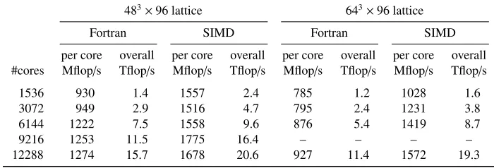
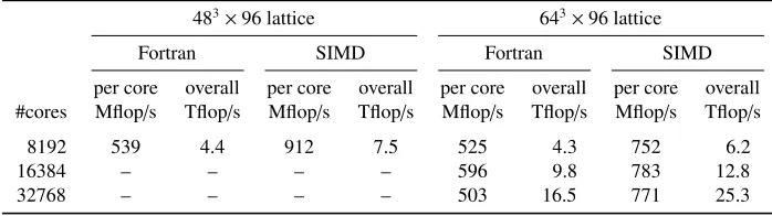
In tables1and2performance figures are listed for machines and lattices that are currently used in production. The optimized code runs between 1.3 and 1.7 times faster.

Table 1.Double precision performance of thecg-solver of BQCD on a Cray XC40 (24 cores per node).

483_×_{96 lattice} ₆₄3_×_{96 lattice}

Fortran SIMD Fortran SIMD

per core overall per core overall per core overall per core overall #cores Mflop/s Tflop/s Mflop/s Tflop/s Mflop/s Tflop/s Mflop/s Tflop/s

1536 930 1.4 1557 2.4 785 1.2 1028 1.6 3072 949 2.9 1516 4.7 795 2.4 1231 3.8 6144 1222 7.5 1558 9.6 876 5.4 1419 8.7

9216 1253 11.5 1775 16.4 – – – –

12288 1274 15.7 1678 20.6 927 11.4 1572 19.3

5.2 QUDA

BQCD can run on GPUs by employing the QUDA library [17]. QUDA has a BQCD interface to its

(5)

References

[1] Y. Nakamura, H. Stüben, PoSLATTICE2010, 040 (2010),1011.0199
[2] H. Stüben (UKQCD, QCDSF), Nucl. Phys. Proc. Suppl.94, 273 (2001),hep-lat/0011045 [3] M. Göckeler et al. (QCDSF), PoSLAT2007, 041 (2007),0712.3525
[4] N. Cundy et al., Phys. Rev.D79, 094507 (2009),0901.3302 [5] R. Horsley et al., JHEP04, 093 (2016),1509.00799
[6] A.J. Chambers et al. (QCDSF/UKQCD, CSSM), Phys. Rev.D90, 014510 (2014),1405.3019 [7] A.J. Chambers et al., Phys. Rev.D92, 114517 (2015),1508.06856
[8] T. Haar, W. Kamleh, J. Zanotti, Y. Nakamura, Comput. Phys. Commun. 215, 113 (2017), 1609.02652
[9] S. Hollitt, P. Jackson, R. Young, J. Zanotti, PoSINPC2016, 272 (2017)
[10] X.Y. Jin, Y. Kuramashi, Y. Nakamura, S. Takeda, A. Ukawa, Phys. Rev.D88, 094508 (2013), 1307.7205
[11] X.Y. Jin, Y. Kuramashi, Y. Nakamura, S. Takeda, A. Ukawa, Phys. Rev.D92, 114511 (2015), 1504.00113
[12] X.Y. Jin, Y. Kuramashi, Y. Nakamura, S. Takeda, A. Ukawa, Phys. Rev.D96, 034523 (2017), 1706.01178
[13] G.S. Bali, S. Collins, A. Cox, A. Schäfer, Phys. Rev.D96, 074501 (2017),1706.01247 [14] https://www.rrz.uni-hamburg.de/bqcd
[15] G. Schierholz, Y. Nakamura,Dynamical QCD+Axion simulation: First results, inProceedings, 35th International Symposium on Lattice Field Theory (Lattice2017): Granada, Spain, to appear in EPJ Web Conf.
[16] T.W. Chiu, T.H. Hsieh, C.H. Huang, T.R. Huang, Phys. Rev. D66, 114502 (2002), hep-lat/0206007