R E S E A R C H
Open Access
Forecasting WiMAX traffic by data mining
methodology
Cristina Stolojescu-Crisan
*and Alexandru Isar
Abstract
One of the most important objectives of wireless network service providers is to make the traffic as uniform as possible in different sectors of the network. In this paper, we analyze the uniformity of the traffic in a WiMAX network with the aid of a forecasting methodology. Taking into account the high volume of data transferred in a wireless network and the requirement of real time, we propose a forecasting methodology based on data mining. The theoretical basis of the proposed method is explained in detail. Its implementation is highlighted by diagrams, which explain each step of the algorithm. The method is applied on real data and the obtained results are discussed.
Keywords: Forecasting; Data mining; Traffic; Wavelets; WiMAX
1 Introduction
Worldwide Interoperability for Microwave Access (WiMAX) technology is a modern solution for wireless networks. One of the most difficult problems that appear in the exploitation of a WiMAX network is the non-uniformity of traffic developed by different base stations. This comportment is induced by the ad hoc nature of wireless networks and concerns the service providers who administrate the network. The amount of traffic through a base station (BS) should not be higher than the capacity of that BS. If the amount of traffic approaches the capacity of the BS, then it saturates. Due to the traffic non-uniformity, different BS will saturate at different future moments. These moments can be predicted using traffic forecasting methodologies.
The traces obtained by the registration of the traffic of each BS composing a WiMAX network are time series. Many approaches involving time series models have been used for traffic forecasting, such as statistical models or models based on neural networks, [1]. For more than two decades, Box-Jenkins autoregressive integrated moving average (ARIMA) technique has been used for time series forecasting. This class of models is used to build the time series model in a sequence of steps which are repeated
*Correspondence: [email protected]
Department of Communications, “Politehnica” University of Timisoara, 2, V. Parvan, Timisoara 300223, Romania
until the optimum model is achieved. Box-Jenkins mod-els can be used to represent stationary or non-stationary processes. ARIMA models are used for traffic forecast-ing in [2,3]. In [2] the authors proposed to model the traffic evolution in an IP backbone network at large time scales. The forecasting method is accelerated by using wavelets, taking into account the sparsity of wavelet coef-ficients. Wavelets can localize data in time scale space. At high scales, wavelets have a small time support and are able to identify discontinuities or singularities, while at low scales wavelets have a larger time support and can identify periodicities. The algorithm of the traffic analysis methodology proposed in [2] is presented in Figure 1.
The methodology supposes the use of ARIMA models in the wavelet domain to estimate the overall tendency and the variability of the time series belonging to a wire-line network traffic database. The first block in Figure 1 implements a multiresolution analysis (MRA), using the stationary wavelet transform (SWT), providing two types of wavelet coefficients: approximation coefficients used for modeling the traffic overall tendency and detail coeffi-cients used for modeling the variability around the overall tendency of traffic. The second block in Figure 1 imple-ments an analysis of variance (ANOVA) procedure, which validates the MRA previously implemented. The third block in Figure 1 establishes the two statistical models for the overall tendency and for the variability of traffic, using ARIMA modeling and Box-Jenkins methodology. Finally,
Figure 1The forecasting methodology proposed in [2].
the last block in Figure 1 estimates the risk of saturation of the considered server.
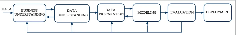
The first goal of the present paper is of methodological nature. We show that the approach presented in [2] can be regarded as a data mining methodology. The WiMAX traffic forecasting method proposed in this paper, inspired by [2], is designed following the Cross Industry Standard Process for Data Mining (CRISP-DM) methodology. Data mining is an analytic process designed to explore and to extract useful information from large data volumes. According to CRISP-DM [4], the process has several steps: business understanding, data understanding, data prepa-ration, modeling, evaluation and deployment. The suc-cession of those phases and their interdependence are represented in Figure 2.
The second goal of this paper is of practical nature. We present the proposed forecasting algorithm, highlighting the differences between the wireline and wireless traffic and the results obtained for a WiMAX database.
The structure of the paper is as follows. In Section 2, the phases of design are described. Section 3 is dedicated to the implementation of the proposed forecasting sys-tem, each sub-system functionality being exemplified by figures. The results obtained applying the proposed fore-casting methodology are presented in Section 4. Finally, Section 5 concludes the paper.
2 The WiMAX traffic forecasting method
In the following, details about the phases of the proposed algorithm in Figure 2 are presented.
2.1 Business understanding
The first phase of a data mining project involves under-standing the objectives and the requirements of the project, defining the problem and designing a preliminary plan to achieve these objectives. The objective of the pro-posed algorithm is to predict when upgrades of a given
BS must take place. We compute an aggregate demand for each BS and we look at its evolution at time scales larger than 1 h. The requirement of the project is to per-form this prediction fast and precise. We have chosen the forecasting methodology proposed in [2], and our prelim-inary plan was to adapt this methodology to the case of a WiMAX network.
2.2 Data understanding
Data understanding phase implies collecting initial data, describing and exploring data. In our case, the data was obtained by monitoring the traffic from 67 BS composing a WiMAX network. The duration of collection is 8 weeks. Our database is formed by numerical values represent-ing the total number of packets/bytes from uplink and downlink channels, for each BS. The values were recorded every 15 min and the traces are accessible in two formats: bytes per second and packets per second. Supplementary details about the database are presented in [5]. We will analyze the format in packets per second, because it is easier to handle time series with smaller values of sam-ples. For estimating the moment when the traffic of each BS becomes comparable with the BS capacity, the down-link channel is more important. The traffic has a higher volume in downlink. Therefore, the results presented in the following correspond to downlink channel. The risk of saturation of the BS in uplink is considerably smaller.
2.3 Data preparation
This phase includes selecting data to be used for analysis and data clearing, such as identification of the potential errors in data sets, handling missing values, and removal of noises or other unexpected results that could appear during the acquisition process. The incomplete or miss-ing data constitute a problem. Despite the efforts made to reduce their occurrence, in most cases missing values can-not be avoided. If the number of missing values is big, the
results are not relevant. It is therefore essential to know how to minimize the amount of missing values and which strategy to select in order to handle missing data. There are several strategies of handling missing data, for exam-ple delete all instances where there is at least one missing value, replacing missing attribute values by the attribute mean, or estimating each of the missing values using the values that are present in the dataset (interpolation) [6]. There are many different interpolation methods such as linear, polynomial, cubic or nearest neighbor interpola-tion. We have chosen the cubic interpolation because for some BS the missing values are situated on the first/last position of the vector and this fact forbids us to use, for example, the linear interpolation.
Next, a multi-time scale analysis is proposed. The SWT is used to decompose the original signal into a range of frequency bands. The level of decomposition (n) depends on the length of the original signal. For a discrete signal, in order to be able to apply the SWT, if the decomposition at levelnis needed, 2n must divide evenly the length of the signal. Levelnof decomposition givesn+1 signals for processing: one approximation signal, corresponding to the current level, andndetail sequences, corresponding to each of thendecomposition levels. The value ofngives the maximal number of resolutions which can be used in the MRA.
WiMAX traffic exhibits some periodicities which are better noticed if the sampling interval is modified from 15 to 90 min. So, by temporal decimation with a factor of 6, these time series can be transformed in signals with a temporal resolution of 1.5 h. This represents the highest time resolution which is used in the proposed MRA. Fur-ther on, these temporal series will be denoted byx(t). The derived temporal seriesx(2pt)have a temporal resolution of 2p×1.5 h.
To extract the overall trend of the traffic time series, the MRA of the temporal seriesx(t), using temporal res-olutions between 1.5 and 96 h, is performed. We used Shensa’s algorithm, which corresponds to the computa-tion of the SWT, with six levels of decomposicomputa-tion. At each temporal resolution, two categories of coefficients are obtained: approximation coefficients and detail coeffi-cients. The overall trend of the traffic time series is better highlighted by the sequence of approximation coefficients obtained at the time resolution of 96 h (corresponding to the sixth decomposition level),a6. In the data mining
context, the separation of the last sequence of approxi-mation coefficients can be regarded as a data preparation operation. The form of this sequence is appropriate for modeling the overall tendency of the traffic, using linear predictive models. The detail sequences reflect the vari-ability of the traffic and have different energies. In the following, the detail sequences corresponding to time res-olutions between 1.5 and 96 h will be denoted byd1−d6.
The equation describing the proposed multi-time scale analysis is:
Computing the energies of the detail sequencesd1−d6,
we observed that the highest energy corresponds tod3
(the time resolution of 12 h). The next detail energy value in decreasing order corresponds to a time resolution of 24 h (the detaild4), where the highest periodicities of the
time series were observed. The energy of the coefficients a6, d3, and d4 represents a great quantity of the
over-all energy of the analyzed time series. The total energy contained inx(t)will be:
E=
∞
−∞|x(t)|
2dt= ||x(t)||2. (2)
Hence, we have decided to ignore the detail sequences with small energies, to reduce the amount of computa-tion and to keep in our multi-time scale analysis only the detailsd3andd4, which explain the deviation of the time
series around its overall trend:
x(t)=a6(t)+βd3(t)+γd4(t). (3)
The model in (3) represents the new statistical model for the traffic time series to be predicted. It reduces the multiple linear regression model in (1) to only two compo-nents: the overall trend of the traffic (described bya6) and
the variability (described by the detail coefficientsd3and
d4). In order to use the new statistical model, the weights
βandγ must be identified. First, for the identification of the weightβ, the contribution ofd4is neglected. The new
statistical model will be expressed by:
x(t)=a6(t)+βd3(t)+e(t), (4)
where e(t) represents the error of the new statistical model.
The optimal value of parameter β can be found by minimizing the mean square ofe(t):
βopt=argmin β
x(t)−a6(t)−βd3(t)2. (5)
The already mentioned search procedure can be used for the computation of the optimal value of γ as well. This time, the contribution of the coefficient sequence,d4,
is taken into account. The new statistical model will be expressed by:
x(t)=a6(t)+βoptd3(t)+γd4(t)+e(t). (6)
The optimal value of parameter γ can be found by minimizing the new mean square ofe(t):
γopt=argmin
γ
For capacity planning purposes, one only needs to know the traffic baseline in the future, along with possible fluc-tuations of the traffic around this particular baseline. Since our goal is not to forecast the exact amount of traffic on a particular day in the future, we calculate the weekly standard deviation as the average of the seven values com-puted within each week. Given that the sequence a6(t)
is a very smooth approximation of the original signal, we calculate its average across each week and we create a new time series, capturing the long-term trend from one week to the next. Approximating the original signal, using weekly average values for the overall long-term trend and the daily standard deviation, results in a model which accurately captures the desired behavior. So, our database is prepared now for modeling the overall tendency of the traffic and the variability around this tendency.
2.4 Modeling
Modeling phase involves the selection of the modeling technique and the estimation of model’s parameters. Our goal is to model the tendency and the variability of the traffic using linear time series models. Let us denote the terms describing the variability with:
dt3(t)=βoptd3(t)+γoptd4(t). (8)
2.4.1 Basic stochastic models in time series analysis In the following, some basic stochastic models in time series analysis are presented.
An autoregressive model of order p (AR(p)) is a weighted linear sum of the past p values [7] and it is defined by the following equation:
Xt=Zt+φ1Xt−1+φ2Xt−2+. . .+φpXt−p, (9)
where Xt represent the time series which the model must establish,φp(.)is apth degree polynomial andZtis a white noise time series.
A moving average (MA) process of orderqis a weighted linear sum of the pastqrandom shocks:
Xt=Zt+θ1Zt−1+θ2Zt−2+. . .+θqZt−q, (10)
whereθq(.)is aqth degree polynomial andZtis a white noise random process with constant variance and zero mean [7].
Being given a time series of dataXt, an autoregressive moving average (ARMA) model is a tool for understand-ing and predictunderstand-ing future values in this series. The model consists of two parts, an AR part and a MA part. The model is usually then referred to as the ARMA(p,q) model, wherepis the order of the autoregressive part andqis the order of the moving average part. A time seriesXt is an ARMA(p,q) process ifXtis stationary and if:
φ (B)Xt=θ (B)Zt, (11)
which can be expressed as:
p
The ARMA model fitting procedure assumes data to be stationary. If the time series exhibits variations that violate the stationary assumption, then there are specific approaches that could be used to render the time series stationary. Most statistical forecasting methods are based on the assumption that the time series can be rendered approximately stationary through the use of mathemat-ical transformations. A stationarized series is relatively easy to predict because its statistical properties will be the same in the future as they have been in the past. The predictions for the stationarized series can then be trans-formed by reversing whatever mathematical transforma-tions were previously used, to obtain predictransforma-tions for the original series. Thus, finding the sequence of transforma-tions needed to stationarize a time series often provides important clues in the search for an appropriate forecast-ing model. One of the operations which can be used for the stationarization of a time series is the differencing operation. The first difference of a time series is the series of changes from one moment to the next. IfY(t)denotes the value of the time seriesYat timet, then the first dif-ference ofY at timetis equal toY(t)−Y(t−1). If the first difference of Y is stationary but correlated, then a more sophisticated forecasting model, such as exponential smoothing or ARIMA may be appropriate.
ARIMA model is a generalization of an ARMA model. In statistics and signal processing, ARIMA models, some-times called Jenkins models after the iterative Box-Jenkins methodology used to estimate them, are usually applied for time series data. ARIMA models are fitted to time series data, either to better understand the data or to predict future points in the series. They are applied in some cases where data show evidence of non-stationarity, when some initial differencing steps must be applied to remove the non-stationarity.
The model is generally referred to as an ARIMA(p,d,q), wherep,d, andqare integers greater than or equal to zero and refer to the order of the autoregressive, integration (number of differencing steps needed to achieve stationar-ity), and moving average parts of the model, respectively:
φ (B)(1−B)dXt=θ (B)Zt. (13)
consists in the degree of differencing d, which for FARIMA models takes real values.
We have selected ARIMA modeling procedure and we have implemented it with the aid of Box-Jenkins methodology.
2.4.2 Box-Jenkins methodology
The Box-Jenkins methodology [9] applies to ARMA or ARIMA models to find the best fit of a time series to its past values, in order to make forecasts. The origi-nal methodology uses an iterative three-stage modeling approach:
• Model identification and model selection. The first goal is to make sure that the time series are stationary. Stationarity can be assessed from a run sequence plot. It can also be detected from an autocorrelation plot. Specifically, non-stationarity is often indicated by an autocorrelation plot with very slow decay. The second goal is to identify seasonality in the dependent series. Seasonality (or periodicity) can usually be assessed from an autocorrelation plot, a seasonal sub-series plot, or a spectral plot.
• Parameter estimation. Once stationarity and seasonality have been addressed, the next step is to identify the order (i.e., thep and q) of the AR and MA parts. The primary tools for doing this are the autocorrelation (ACF) plot and the partial
autocorrelation (PACF) plot. The sample ACF plot and the sample PACF plot are compared to the theoretical behavior of these plots, when the order is known. Specifically, for an AR(1) process, the sample ACF should have an exponentially decreasing appearance. However, higher-order AR processes are often a mixture of exponentially decreasing and damped sinusoidal components. The ACF of a MA(q) process becomes zero at lagq+1and greater, so we examine the sample ACF to see where it essentially becomes zero.
• Model checking by testing whether the estimated model conforms to the specifications of a stationary univariate process. In particular, the residuals should be as small as possible and should not follow a model. If the estimation is inadequate, we have to go back to step one and attempt to build a better model.
The determination of an appropriate ARMA(p,q) model to represent an observed stationary time series involves the orderpandqselection and estimation of the mean, the coefficientsφpandθq, and the variance of the white noise, σ2. Whenpandqare known, good estimators ofφ and θ can be found by imagining the data to be observations of a stationary Gaussian time series and maximizing the likelihood with respect to the parametersφp,θq andσ2. The estimators obtained using this procedure are known
as maximum likelihood estimators (MLE). The aim of this method is to determine the parameters that maximize the probability of observations. A detailed theoretical approach regarding MLE is presented in [10].
In the following, the problem of selecting appropriate values for the ordersp andq will be discussed. Several criteria have been proposed in the literature, since the problem of model selection arises frequently in statistics [11].
Developed by Akaike in 1969, final prediction error (FPE) criterion is used to select the appropriate order of an AR process to fit to a time seriesX1,. . .,Xn. The most accurate model has the smallest FPE. The FPE for an AR process of orderpcan be estimated according to the following equation:
FPE= ˆσ2·n+p
n−p, (14)
wherenis the number of samples andσˆ2is the estimated noise variance.
The Akaike information criterion (AIC) is a measure of the goodness of fit of an estimated statistical model. In fact, AIC is the generalization of maximum likelihood principle. Given observations X1,. . .,Xn of an ARMA process, the AIC statistic is defined as:
AIC= −2·ln(L)+2(p+q+1), (15)
whereLis the likelihood function.
The corrected AIC (AICC) is a bias-corrected version of the AIC, proposed in [10]. This criterion is applied as follows: choosep,q,φp, andθqto minimize:
AICC= −2·lnL+ 2(p+q+1)n
n−p−q−2, (16)
wherenis the number of samples.
In the case of AICC and AIC statistics, forn→ ∞, the factors 2(p+q+1)n/(n−p−q−2)respective 2(p+q+1) are asymptotically equivalent.
The Bayesian information criterion (BIC) is another cri-terion for model selection, used to correct the overfitting nature of the AIC [10]. For a zero-mean causal invert-ible ARMA(p,q) process, BIC is defined by the following equation:
where σˆ2 is is the maximum likelihood estimator of σ2 (the white noise variance of the AR(p) model).
possible and exhibit no patterns [9]. The residuals repre-sent all the influences on the time series which are not explained by other of its components (trend, seasonal component, trade cycle). The steps involved to build the model are repeated in order to find a specific multiple times formula that copies the patterns in the series as closely as possible and produces accurate forecasts. The input data must be adjusted first to form a stationary series and next, a basic model can be identified [9]. The initial model can be selected using Matlab functionidpoly.
2.5 Evaluation
One of the most important phases of a data mining project is the evaluation phase, which collaborates with all the precedent phases. The connection with data preparation phase supposes the evaluation of the MRA, using ANOVA (see Figure 1).
2.5.1 Analysis of variance
ANOVA is a statistical method used to quantify the amount of variability accounted by each term in a multi-ple linear regression model. It can be used in the reduction of a multiple linear regression model process, identifying those terms in the original model that explain the most significant amount of variance.
The sum squared error (SSE) is defined as:
SSE= n
t=1
e(t)2, (18)
wheree(t)represents the error of the model. We denote the following sum with SSX:
SSX= n
t=1
y(t)2, (19)
wherey(t)is the observed response of the model.
The total sum of squares (SST) is defined as the uncer-tainty that would be present if one had to predict individ-ual responses without any other information:
SST=
The ANOVA methodology splits this variability into two parts. One component is accounted for by the model and it corresponds to the reduction in uncertainty that occurs when the regression model is used to predict the response. The remaining component is the uncertainty that remains even after the model is used. The regression sum of squares, SSR, is defined as the difference between SST and SSE. This difference represents the sum of the squares explained by the regression.
The fraction of the variance that is explained by the regression determines the goodness of the regression and is called coefficient of determination,R2:
R2= SSR
SST. (21)
The model is considered to be statistically significant if it can account for a large fraction of the variability in the response, i.e. yields large values forR2.
2.6 Deployment
The final stage, deployment, involves the application of the model to new data in order to generate predictions. A statistical model is aggregated for each BS using the corre-sponding overall tendency and variability models and its trajectory is established. The saturation moment can be found at the intersection of this trajectory with a horizon-tal line which represents the BS saturation threshold.
3 Implementation
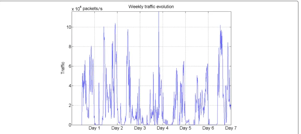
We will exemplify in the following the stages of the pro-posed forecasting method, using an example of a par-ticular trace (corresponding to BS1). We will begin with the data preparation stage. The simple plot of the traffic curves shows the existence of periodicities in the traffic. In Figure 3 the traffic evolution during 1 week, randomly selected for BS1, is presented.
In order to verify the existence of periodicities, we calculated the Fourier transform of the signal and we analyzed the power spectral density in Figure 4. We can remark, in Figure 4, the eighth harmonic which corre-sponds to a period of 24 h. The dominant period across all traces is the 24 h one. The trace in Figure 4 has been arbitrarily chosen. There are other traces in the database for which the eighth harmonic is dominant, being several times bigger than the other harmonics and proving the periodicity with the period of 24 h of the traffic. However, depending on the trace, the periodicity with the period of 24 h can also be hidden. This periodicity has social rea-sons, reflecting a pattern of diurnal comportment of the network. Such seasonal behavior is commonly observed in practical time series.
Next, we will consider a traffic curve recorded during 8 weeks, represented in Figure 5 with blue.
The representation contains specific underlying overall trend, represented in red. The other two curves represent the deviation, plus (in green)/minus (in black), from the approximation signal. It can be observed that a large part of the traffic is contained between the green and black lines. The red line indicates an increase of the traffic in time, suggesting the possibility of saturation of BS1.
Figure 3A curve describing the weekly traffic evolution for a BS arbitrarily selected.
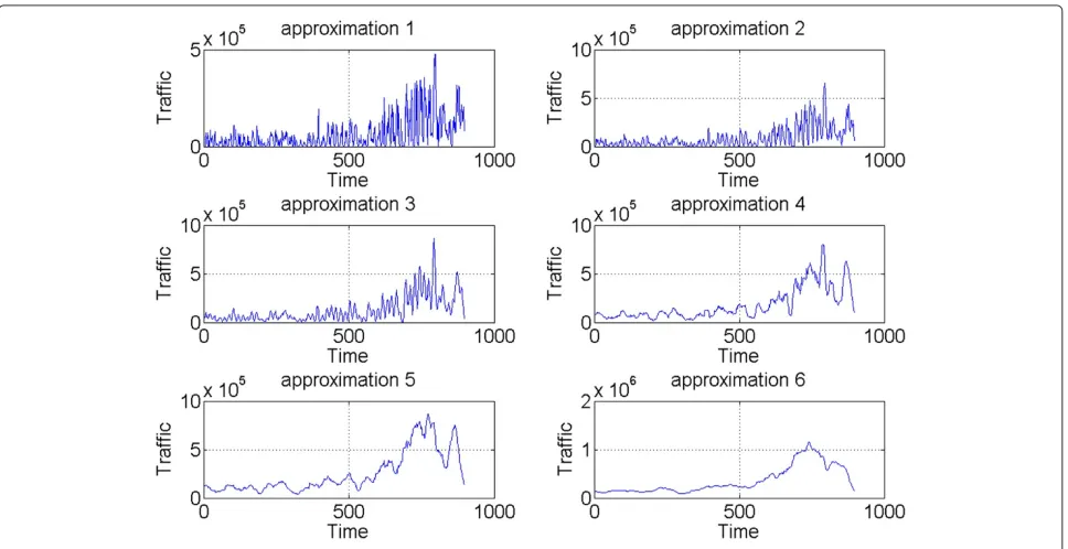
coefficients for six levels of decomposition are shown in Figure 6.
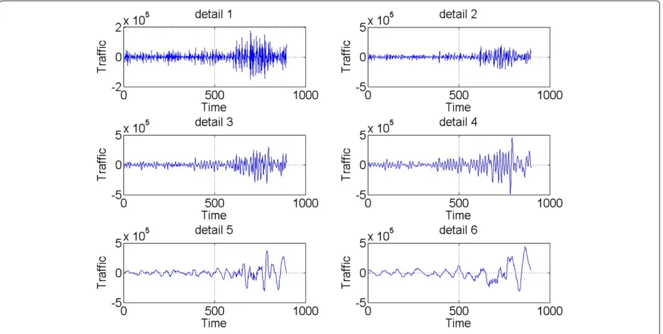
It can be observed that with a higher level of decom-position, the sequence of approximation coefficients becomes more smoothed. The sequences of detail coef-ficients for six levels of decomposition are depicted in Figure 7.
One of the goals of the multi-time scale analysis is to reduce the amount of data, by rejecting some detail coef-ficient sequences, without compromising the precision of the forecast. The result of this step is the new statistical
model of the traffic in Equation 3. It involves the identifi-cation of parametersβ andγ, as it is shown in Equations 5 and 7. In Figures 8 and 9, the minimization procedures described in Equations 5 and 7 are highlighted.
The reconstruction of the original traffic (first plot) using the estimation of the overall trend (realized using a6) and the estimation of the variability (realized using
βd3-second plot andβd3+γd4-third plot) are presented
in Figure 10.
The approximation errors are higher in the second plot than in the third plot. This remark justifies the utilization
Figure 5A traffic curve recorded during 8 weeks, its long-term trend (a6(t)) and deviations froma6(t).
of both weightsβandγ. The approximation in the second plot is smoother than the approximation in the third plot. So, the utilization of the weightγ diminishes the high-frequency components of the errors.
As it was already mentioned, for a long-term forecast-ing, we have computed averages across each week for the terms from the right side of the model in Equation 3. The resulting signal is presented in Figure 11 with red colour. It can be observed that this signal represents a good approximation of the overall tendency of the traffic.
The next step consists in modeling. We used the Box-Jenkins methodology [9] to fit linear time series models, separately for the overall trend and for the variability, starting with the estimations in Figure 11. The estima-tions ‘mean approximation plus’ and ‘mean approximation minus’ are used for modeling the variability, while the esti-mation ‘approxiesti-mation per week’ is used for modeling the overall trend.
In the following, we will present an example to show how the Box-Jenkins methodology for WiMAX traffic
Figure 7The detail coefficient sequences.
prediction is applied. In Figure 12, the approximation coefficients (a6) and their first and second differences are
presented.
The first step is to study which of these sequences are stationary, in order to establish the value of the param-eter d. The correlations of the signals in Figure 12 are represented in Figure 13.
The correlation of a stationary sequence must vanish after few samples. Analyzing Figure 13, we can observe that the third sequence (from up to bottom) has the higher decreasing speed. It has a peak in its middle. The sample
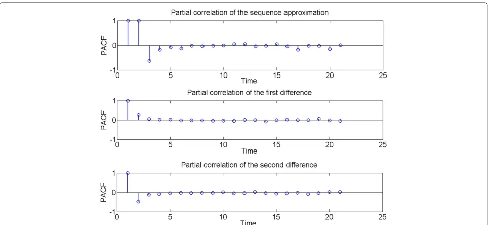
values fall rapidly at the left and the right of this pick, becoming close to zero. This decrease is faster than the one observed in the middle plot in Figure 13 or in the upper plot. The PAC of the signals in Figure 12 are repre-sented in Figure 14. They are also useful for the estimation of orderspandq.
Analyzing Figure 14, we obtain the same conclusion as in the case of Figure 13. The sequence obtained by com-puting the second difference of the sequence of approx-imations is more stationary than the sequence obtained by computing the first difference of approximations or
Figure 9The search of the best value ofγ.
than the sequence of approximations itself. In fact, in [9] it is devised to apply the Box-Jenkins methodology two times. First, an initial model is established and then it is optimized in the second run. To initialize the Matlab Box-Jenkins methodology (the functionbj.m), some infor-mation is required: the data to be modeled (one of the three sequences: the approximationc6, its first difference,
or its second difference, in our case) and the model (the valuespandqand the initial coefficients of the polyno-mialsφof orderpandθ of orderq) to be initialized. The results of the functionbj.mrepresent the optimal values of coefficients of the polynomialsθ andφ(which permit
the mathematical description of the model), the degree in which the model fits the data (it must be as small as pos-sible), and the value of FPE which must be as small as possible. The orderspandqof the polynomialsφ andθ can be identified based on their coefficients but the value of the parameter d from the ARIMA model cannot be identified using the function bj.m. For this reason it is identified based on stationarity tests.
One of the most important stages of the proposed WiMAX traffic forecasting methodology is the evaluation. In this phase, both models (for overall tendency and vari-ability of the traffic) are evaluated and all the precedent
Figure 11The average weekly long-term trend and the average daily standard deviation within a week.
steps are reviewed. In order to see if the new statisti-cal model in (3) is representative, we used ANOVA and we computed the coefficient of determination. We have obtained good results for each BS for both statistical mod-els, applying the forecasting algorithm to all the downlink traces from the database and obtaining statistically sig-nificant ARIMA models for each traffic overall tendency and variability of each BS. We have identified the model parameters (pandq) using MLE. The best model was cho-sen as the one that provides the smallest AICC, BIC and FPE while offering the smallest mean square prediction error for a number of weeks ahead.
The last stage of the proposed forecasting methodol-ogy consists in deployment. The models obtained for the long-term trend of the downlink traces from the database indicate that the first difference of those time series is con-sistent with a simple MA model (p=0) with one or two terms (q = 1 and d = 1 orq = 2 and d = 1) plus a constant valueμot. Similar results were obtained for the models of variability of the traffic.
The moment when the saturation of the BS takes place can be predicted comparing the trajectory of the over-all traffic forecast with the BS’s saturation threshold, as shown in Figure 15.
Figure 13Autocorrelations of sequence approximation (first line), their first (second line) and second (third line) differences.
The need for one differencing operation at lag one and the existence of termμot across the model indicate that the long-term trend of the downlink traffic is a simple exponential smoothing with growth. The trajectory for the long-term forecasts will be a sloping line, whose slope is equal toμot. Similar conclusions can be formulated for the variability of the downlink traffic. The trajectory for the variability forecast is a sloping line as well, but it has a much smaller slope. The sum of these sloping lines is a third line, parallel with the trajectory of the long-term forecast, which represents the trajectory of the overall
forecast. Hence, the risk of saturation of a BS is propor-tional with the slope of its overall tendency. Given the estimates of μot across all models, corresponding to all BS, we can conclude, based on the positive values of those slopes, that all traces exhibit upward trends, but grow at different rates.
4 Results
The slope of the overall tendency line in Figure 15 is equal toμot. Analyzing Figure 15, it can be observed that a BS
Figure 15The trajectory for the long-term forecasts.
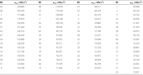
saturates faster ifμot has a higher value. Indeed, for the same value of the saturation threshold, with the growth of μot, the value ofts(which indicates the moment of satu-ration in Figure 15) will decrease. So, the value ofμot is proportional with the saturation risk of the considered BS. In Table 1, a classification of BS in terms of the satura-tion risk is presented. More precisely, the BS are listed in decreasing order of the slope of the overall tendency of their traffic. For BS50, the value ofμot was estimated as
equal to 2.06×1016bits/s2. The results obtained for BS50 are not relevant because a lot of data are missing in the corresponding trace, the interpolation process becoming not reliable. The BS shown on the first column in Table 1 have high values of μot. This means that these BS have a higher risk of saturation than the other ones. The BS with the highest risk of saturation are the following: BS63, BS60, BS3, BS49, BS61. These are the BS which must be upgraded first. The moment,ts, when the upgrade must
Table 1 BS risk of saturation
BS μot(Mb/s2) BS μ
ot(Mb/s2) BS μot(Mb/s2) BS μot(Mb/s2)
63 239.860 48 114.810 13 68.311 1 45.068
60 185.470 52 110.250 53 66.329 2 44.729
3 177.680 8 109.040 6 65.579 9 43.102
49 176.070 7 105.240 5 63.415 42 42.878
61 164.030 56 104.720 26 59.885 33 41.441
57 157.260 55 99.920 12 58.708 30 41.395
62 146.310 65 99.174 39 57.789 28 39.973
67 144.630 20 97.943 38 57.675 41 38.129
54 143.880 29 97.655 35 54.498 40 33.587
18 138.230 46 93.711 37 53.458 36 32.224
64 134.220 10 91.557 23 52.729 25 30.601
16 131.730 19 83.567 45 51.019 15 29.400
59 130.530 43 79.215 22 50.872 11 27.622
58 130.350 44 78.572 24 49.404 31 26.144
51 123.960 66 74.149 27 46.704 17 25.052
4 118.100 14 71.564 47 45.879 21 24.614
Figure 16The proposed forecasting methodology.
take place can be computed using the values ofμotand the values of the BS capacity, as it can be seen in Figure 15.
The base stations with the smallest risk of saturation are BS15, BS11, BS31, BS17 and BS21. Comparing the results in Table 1, it can be observed that the risk of saturation of BS63 is ten times bigger than the risk of saturation of BS21. So, the traffic of different BS is far to be uni-form. This is a significant result because it shows the existence of some limitations in the design of WiMAX networks. This design is based on the Shanon commu-nications theory, which does not take into account some particularities of the wireless networks, for example their ad hocnature, or the effects of different social influences. The traffic analysis presented in this paper is useful for network designers and administrators, being one of the first studies on WiMAX traffic forecasting subjects.
5 Conclusions
We have argued that the traffic forecasting methodology proposed in [2] can be regarded as a data mining method-ology and can be adapted for WiMAX traffic prediction. We have observed that the principal difference between the wireline traffic considered in [2] and the WiMAX traf-fic consists in the higher variability of the wireless traftraf-fic. So, the adaptation of the traffic forecasting methodology presented in Figure 1, in the case of the wireless traffic, consists in the optimization of the ANOVA procedure, as can be seen in Figure 16 (we considered a second param-eter,γ, and we enphasized this modification using the red circle).
This optimization is described in Equation 7. Because, in the case of WiMAX traffic, we have obtained smaller energy values for the sequenced3than the corresponding
values obtained in [2], we have additionally considered the sequenced4.
The proposed forecasting methodology extracts the traffic trends from historical measurements and can iden-tify the BS which exhibits higher growth rates and, thus, may require additional capacity in the future. It is capable of isolating the overall long trend and identifying the com-ponents that significantly contribute to its variability. Pre-dictions based on approximations of those components provide accurate estimates with a minimal computational overhead. All our forecasts were obtained in seconds. All the procedures described are implemented as Matlab functions. We have found that the BS of the considered
network are more charged in downlink cycles than in uplink cycles. This unbalanced comportment gives some indications about the user needs, and its analysis can give useful information for the local operators, regarding the number of users at different locations within the network. We cannot come up with a single WiMAX network-wide forecasting model for the aggregate demand. Different parts of the network grow at different rates (long-term trend) and experience different types of variation (devia-tion from the long-term trend). This comportment prove that other methods must be applied to make the traffic uniform. For example, it could be possible to optimize the positions of some BS [12].
This paper presents one of the first attempts to forecast the traffic of a WiMAX network. Taking into account the high speed of traffic analysis developed by the proposed method (it works practically in real time), we consider that it could be implemented by each WiMAX network service provider.
Competing interests
The authors declare that they have no competing interests.
Received: 29 July 2013 Accepted: 23 November 2013 Published: 6 December 2013
References
1. Z Rong, CR Qiu, X Xia, W Guoping, A case-based reasoning system for individual demand forecasting, inProceedings of the 4th International Conference on Wireless Communications, Networking and Mobile Computing (WiCOM)(IEEE, Piscataway, 2008), pp. 1–6
2. K Papagiannaki, N Taft, Z Zhang, Diot C, Long-term forecasting of internet backbone traffic: observations and initial models, inProceedings of the IEEE INFOCOM(IEEE, Piscataway, 2003), pp. 1178–1188
3. NK Groschwitz, Polyzos G C, A time series model of long-term NSFNET backbone traffic. Proc. IEEE Int. Conf. Commun.3, 1400–1404 (1994) 4. P Chapman, Clinton J, Kerber R, Khabaza T, Reinartz T, Shearer C, Wirth R,
CRISP-DM 1.0 Step-by-step data mining guide (2000). ftp://ftp.software. ibm.com/software/analytics/spss/support/Modeler/Documentation/14/ UserManual/CRISP-DM.pdf. Accessed Nov 2013
5. Stolojescu C, Cusnir A, Moga S, Isar A, Forecasting WiMAX BS traffic by statistical processing in the wavelet domain, inProceedings of IEEE International Symposium on Signals, Circuits and Systems(Iasi, 9–10 July 2009), pp. 177–180
6. L Rokach, Maimon O,The Data Mining and Knowledge Discovery Handbook: A Complete Guide for Researchers and Practitioners(Springer, New York, 2005)
7. C Chatfield,Time-Series Forecasting(Chapman and Hall/CRC Press, Boca Raton, 2000)
8. HZ Moayedi, M Masnadi-Shirazi, ARIMA model for network traffic prediction and anomaly detection, inProceedings of the International Symposium on Information Technology(IEEE, Piscataway, 2008), pp. 1–6 9. GEP Box, GM Jenkins, G Reinsel,Time-Series Analysis: Forecasting and
10. CM Hurvich, Tsai C L, Regression and time series model selection in small samples. Biometrika.76, 297–307 (1989)
11. PJ Brockwell, RA Davis,Introduction to Time Series and Forecasting
(Springer, New York, 2002)
12. C Stolojescu, S Moga, P Lenca, P Isar, WiMAX traffic analysis and base stations classification in terms of LRD. J. Expert Syst.30(4), 285–293 (2013) doi:10.1186/1687-1499-2013-280
Cite this article as:Stolojescu-Crisan and Isar:Forecasting WiMAX traffic by data mining methodology.EURASIP Journal on Wireless Communications and
Networking20132013:280.
Submit your manuscript to a
journal and benefi t from:
7Convenient online submission 7Rigorous peer review
7Immediate publication on acceptance 7Open access: articles freely available online 7High visibility within the fi eld
7Retaining the copyright to your article