Joint scheduling and power control for multicasting in cellular wireless networks

(1)

R E S E A R C H

Open Access

Joint scheduling and power control for

multicasting in cellular wireless networks

Izhak Rubin

1*

, Choo-Chin Tan

1

and Reuven Cohen

2

Abstract

We consider a cellular wireless network. Our aim is to develop adaptive-power scheduling algorithms that enable area base stations to coordinate, on a time-division basis, the transmission of multicast packets to identiﬁed client nodes, for scenarios under which a prescribed code rate is employed. Such mechanisms can be implemented by 4G long term evolution (LTE) systems using multimedia broadcast multicast services (MBMS), meshed WiFi networks, or mobile backbone based ad hoc wireless networks. We show that the joint scheduling and power control problem can be represented as a mixed-integer linear programming model, which is NP-hard. Consequently, we present three heuristic algorithms of polynomial complexity for solving the problem in a practical manner. For small network layouts, our centralized heuristic algorithm is shown to achieve a throughput rate performance that is close to that attained by the optimal scheme. All three of our heuristic algorithms are shown to yield excellent throughput rate performance behavior. The use of power adaptations, when compared with ﬁxed transmit power operations, leads to enhanced throughput rate performance while also lowering communications energy consumption levels.

Comparisons with LTE MBMS over single frequency network based schemes have shown our algorithms to oﬀer enhanced spectral eﬃciency performance, while providing high client coverage.

Keywords: Long term evolution, Multimedia broadcast/multicast services, Multicast, Scheduling, Power control, Spectral eﬃciency

Introduction

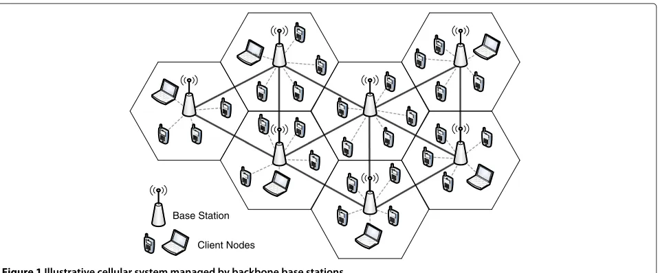
Eﬃcient multicasting of messages in multimedia cellu-lar networks to identiﬁed multicast group clients is a task of primary importance. Consider a wireless cellular network that consists of base stations that are intercon-nected through a backbone network, such as a long term evolution (LTE) system as shown in Figure 1. Messages targeted for multicast distribution are delivered across the backbone by content providers to base stations with clients that belong to the underlying multicast group. In this article, we study the coordinated adaptive-power scheduling of transmissions of such multicast packets by area base stations. The developed schemes are used by neighboring base stations to time-share their downlink channels over a prescribed frequency band. For applica-tion to LTE systems, such an operaapplica-tion is supported by

*Correspondence: [email protected]

1Electrical Engineering Department, University of California, Los Angeles, CA, USA

Full list of author information is available at the end of the article

the multimedia broadcast and multicast service (MBMS) [1,2]. Our scheduling schemes are also highly eﬀective when applied to meshed WiFi networks, or to mobile backbone based ad hoc wireless networks, whereby the roles of base stations are undertaken by access points or backbone nodes, respectively.

Under LTE MBMS, neighboring base stations may engage in coordinated time-synchronized point-to-multipoint transmissions. Client nodes may realize macro-diversity gains through selective combining or soft combining [2,3]. Under a selective combining scheme used by MBMS over single frequency network (MBSFN), multiple MBMS group base stations may be scheduled to transmit the same message at the same time, at the same rate, using the same modulation/coding scheme (MCS), to produce MIMO-type gains at receiving client nodes. Such an MBSFN operation requires strict sym-bol synchronization among base stations, thus imposing spatial conﬁgurational limitations, and increasing imple-mentational complexity and costs [2,4,5]. In addition to

(2)

Base Station

Client Nodes

Figure 1Illustrative cellular system managed by backbone base stations.

combining operations, coordinated scheduling operations can also be performed across neighboring cells to manage inter-cell interference [6,7].

In avoiding the use of such combining operations, the scheduling mechanisms developed in this article ensure each multicast transmission to be successfully received by all identified client nodes at targeted error rates, and thus at acceptable signal-to-interference-and-noise ratio (SINR) levels. Using the algorithms developed in this article over LTE MBMS implementations, point-to-multipoint transmissions can be carried out by base stations, in a time-coordinated fashion, across shared OFDM-based downlink channels, rather than using the MBSFN downlink structure. Such an implementation offers the following advantages: (i) different cells may con-tain different mixes of multicast client groupings. Thus, a base station that does not have clients that belong to a certain multicast group would not be configured to mul-ticast (at the same time slot) packets that belong to this group for the sole purpose of achieving combining gains at client nodes of nearby base stations. This reduces energy consumption and increases spectral utilization efficiency; (ii) client nodes are not required to engage in MIMO-type (multipath combining oriented) operations, enabling the efficient operation of smaller user equipment, such as sen-sors and handheld smart phone platforms. A wide range of schemes have been proposed to find the optimal link scheduling with power control for unicasting in spatial-TDMA networks [8-10]. Adaptive power control has been utilized by energy-aware multicasting schemes to synthe-size a multicast structure that minimizes the total energy cost [11,12]. However, to the best of our knowledge, we have found no published articles that solve the scheduling problem jointly with adaptive power control for multi-casting in wireless cellular networks, under which base

stations share their downlink channels on a coordinated spatial-TDMA basis.

The objective of this article is to develop efficient algo-rithms for such an operation and investigate the extent of throughput enhancement that can be feasibly attained. We first model the problem as a mixed-integer linear pro-gramming problem to find an optimal solution, and con-clude that the problem is NP-hard. We then present three computationally efficient heuristic algorithms that jointly determine the multicast schedule, the underlying base sta-tion transmit power levels and the set of client nodes that are addressed by each transmitting base station in each time slot. Consequently, a scheduled base station can make effective use of its allocated time slots to success-fully transmit any mix of unicast and multicast packets. For scheduling unicast traffic, time slots allocated to a base station do not need to be re-negotiated and re-configured (hence reducing the ensuing rate of control traffic) as long as its mobile client nodes continue to reside in the geo-graphical region that is targeted for coverage during the allocated time period. The presented algorithms can be readily extended to operations under which base stations use sectorized antennas. Each scheduled downlink trans-mission is then targeted to cover a sector zone, rather than a disk-shaped geographical region.

(3)

our schemes in comparison with the corresponding per-formance behavior of illustrative LTE MBSFN systems. Conclusions and future works are presented in Section “Conclusions”.

System model

We consider a cellular wireless network that consists of base stations with omni-directional antennas. Client nodes located in a cell region communicate through the base station with which they associate. We assume that the transmissions of multicast packets are scheduled over a prescribed frequency band, using a ﬁxed transmit rate achieved under a prescribed MCS. Neighboring base sta-tions are time-slot synchronized. They share their down-link channels on a coordinated spatial-TDMA basis. The time-slot duration is assumed to be equal to the transmis-sion time of a prescribed load of packets, incorporating a suﬃciently long preamble that compensates for incurred propagation delays.

Under our centralized algorithm, a scheduling con-troller is used to allocate time slots to base stations for the transmission of multicast messages. The controller periodically collects channel quality information (CQI) from client nodes, and uses the data to form a channel gain matrix for each downlink channel. The CQI collec-tion mechanism is part of the LTE infrastructure, and is included in the control plane [13]. We assume here that such updates are executed at a suﬃciently fast pace to be of relevance for the time period over which the under-lying slot allocation operation is performed. During this period of time, we assume the locations of client nodes and the corresponding downlink transmission gain val-ues to be essentially static. Base station i is capable of adjusting its transmit power continuously in a given range [0,Pmax(i)], in a slot-by-slot fashion. For the special case in which all base stations are limited by the same maximum power level, we denote the latter asPmax. Further adap-tations can be carried out through the dynamic setting of the MCS and its ensuing code rate to attain performance upgrade; however, the purpose in this article is to deter-mine the contributions made by the sole use of transmit power adaptations on the performance behavior of multi-cast scheduling mechanisms. Moreover, the setting of the data rate (based on the MCS conﬁguration) in the multi-casting scenario is dictated by constrains imposed by the critical client nodes of a multicast transmission, i.e. the most interference-prone client nodes within the multicast group.

Client nodes are initially associated with one of the base stations in the underlying network by selecting the one from which they receive a control signal at the highest power level. As the scheduling operation progresses, when a base station is selected for transmission at a given time slot, the boundary clients of the base station’s neighboring

cells may be able to receive multicast packets from the selected base station (depending on surrounding interfer-ences and the SINR requirements at the client nodes). These boundary clients are then scheduled to receive the underlying multicast packets from such a base station, and are then ‘removed’ as multicast clients of their respec-tive initial-associated base stations. We identify such an assignment as a multicast re-linking (m-linking) opera-tion. The performance improvement under the m-linking process is thus related to the increase in the geographical coverage span that is attained (so that in the underly-ing time slot, additional client nodes, the re-linked ones, are also accommodated), and the consequent reduction in coverage scope that may be required of residual base stations.

For a unicast transmission scenario, a directed commu-nication link lij is established from node i to node j if there exists a power levelP∈[ 0,Pmax(i)], under which the SNR level measured at the receiver of node jexceeds a prescribed threshold levelγ (j); i.e.,

GijP

η≥γ (j) (1)

where Gij denotes the propagation gain incurred dur-ing the transmission, and η is the thermal noise power monitored at node j (which, without loss of generality, is assumed to be the same for all nodes). Such a model is often identified as the SINR-based interference model [14]. The value of the thresholdγ (j)depends on the pre-scribed block link error rate (BLER), MCS and ensuing data rate (or spectral efficiency) used by nodej[15]. We henceforth assume in this article that a specific MCS is employed, so that under a prescribed BLER level for the link terminating at receiver j, the corresponding mini-mum acceptable SINR level is denoted asγ (j). To simplify our algorithmic schemes, we further assume here that γ (j) =γ for each nodej. Consequently, each scheduled base station will transmit its packets in its allocated slots at a prescribed data rate.

For a multicasting scenario, let NTx represents the set of base stations with multicast messages to dis-tribute and NRx denotes the set of client nodes inter-ested in the underlying multicast packets. Let G=

Gikjk, ik ∈NTx, jk ∈NRx(ik)

represents the propaga-tion gain matrix andNRx(ik)denotes the subset of client nodes that is associated with base stationik (BS-ik). Let

ik → NRx(ik) and Pi(kt), P (t)

ik ∈[ 0,Pmax(ik)] represent a

multicast transmission by BS-ik that reaches the entire group of multicast client associated with this base station, and the corresponding transmit power level in time slot

(4)

be received at each of its client node with an SINR level that is higher than a prescribed threshold. Hence, for each BS-ik, considering all the multicast client nodes that are currently linked with it, we require:

GikjkP that satisﬁes the system of linear inequalities in Equation (2) in its equality form, when it exists, is referred to as the apex solution. If S(t) is a feasible transmission sce-nario under P¯AP(t), then any other power vector P¯(t) under whichS(t) is feasible would require at least as much power (i.e., P¯(t) ≥ ¯PAP(t) component-wise). Based on Perron–Frobenious theorem [16,17], it is shown that if a transmission scenarioS(t) is feasible, the apex solution of the corresponding system of linear inequalities is strongly Pareto optimal with respect toS(t). Thus, this is an energy eﬃcient solution; the apex point yields a solution that employs the lowest power level for each base station.

The number of multicast packets per frame required to be transmitted by base stations with multicast messages to distribute is assigned by the upper layer operations and is determined by the statistics of total oﬀered load and the desired delay-throughput performance metrics. These calculations produce the requirement ofWikpackets to be

multicasted per frame for every BS-ik, whereik ∈ NTx. Using adaptive power control jointly with scheduling, we aim to design a time frame with the shortest schedule length to reach all of the respective multicast clients. The solution speciﬁes the schedule, identifying in each time slot the set of transmitting base stations, their trans-mit power levels and the set of client nodes that each base station aims to reach. We also strive, as a secondary consideration, to employ a power eﬃcient solution.

MILP model

In this section, we develop and investigate a MILP formu-lation for the joint adaptive-power multicast scheduling problem. We assume that the initial associations between clients and their base stations are determined based on a prescribed routine, such as that noted above, under which a client associates with the base station whose signal is received at the highest power level. The input for the opti-mization model is the set of designated base stations with multicast messages to distribute (NTx), the sets of mul-ticast clients with their associated BS-ik (NRx(ik), ik ∈

NTx), the traﬃc matrix, the propagation gain matrix (G), maximum transmit power of each BS-ik (Pmax(ik)), min-imum required received SINR (γ (jk)), and thermal noise

power levels impacting the receivers of client nodes (η). To determine the system’s throughput capacity level attain-able under the employed scheduling scheme, we assume the allocated multicasting period to include a suﬃcient number of time slots to accommodate the multicast load targeted for this period, so that the required time frame duration is upper bounded by a ﬁnite duration Tmax. The decision variables for the optimization algorithm are {X_i(t)

The solution of the scheduling problem is represented as (X,P). The set of quadratic constraint:

where is a suﬃciently large positive number, imposes the SINR requirement for a base station multicast trans-mission at time slott. Note that if no transmission by BS-ik is scheduled to take place at time slott(X_i(t)

k =0), the

asso-ciated constraint becomes redundant. We next show that this scheduling problem can be modeled as the following MILP formulation:

In Equation (5),εis a suﬃciently small positive number, andctis a positive constants deﬁned as

(5)

It can be seen that the constraints expressed by Equation (6) guarantee that a multicast transmission by BS-ik will reach all the multicast clients under its management. The coeﬃcients{ct}are used to ensure that the length of the schedule corresponding to the optimal solution of the MILP formulation is minimal, whereas the positivity of ε ensures the strongly Pareto optimality of the optimal transmit power levels deduced from the optimum solution of the MILP formulation.

Lemma 1.Every MILP solution yields a feasible trans-mission scenario at each time slot.

Proof.Consider an arbitrary time slot t under a fea-sible solution (X,P) of the MILP formulation, where

X =

, is feasible. For a transmission ik →

NRx(ik) in S(t), sinceXi(kt) = 1, based on Equation (6),

which along with the transmit power constraint in Equation (7) conﬁrms the feasibility of each transmission inS(t). Consequently, transmission scenarioS(t) is feasible under power vectorP¯(t). QED

The joint power control and scheduling problem for unicast transmissions, as presented in [9], can be reduced to an edge coloring problem, which is NP-hard [18]. Adding in the multicast nature of our problem, which induces further complexity since a single base station transmission has to satisfy the minimum SINR require-ment imposed for each one of its multicast clients, implies that the underlying scheduling problem is also NP-hard. We therefore conclude the need for developing heuristic algorithms to provide solution schemes to this adaptive-power scheduling problem that is computationally eﬃ-cient and scalable, when considering networks that may include a large number of base stations and client nodes.

Heuristics algorithms for joint power control and multicast scheduling

We ﬁrst introduce the notion of a power control mul-ticast interference graph [9], which is used as the basic building block for our heuristic Algorithm 1. Consider a scenario with only two base stations, BS-i1 and BS-i2, with corresponding sets of multicast clientsNRx(i1) and NRx₍_i

2). The transmission scenario S(t) = {i1 → NRx(i1),i2 → NRx(i2)}is feasible if and only if the coor-dinates of the apex power vector solution of the following linear inequalities are in the range(0, 0) ≤ P_i(t)

To reduce the computational complexity of Equation (13), we employ an approximation technique. Instead of inspecting the SINR condition for all multicast clients at each base station, we consider for each pair of such base stations a pair of critical client nodes, one such node in each cell. Client nodes monitor their received interference power levels and report them to their base stations peri-odically via CQI updates. By using CQI data collected by the base stations (or centralize scheduling controller), crit-ical client nodes are then identiﬁed to be those nodes that are measured to experience the most interference (rela-tive to the interference signals that are generated). We denote these critical nodes for BS-i1and BS-i2asj∗₁andj∗₂, respectively. Assume transmissionsi1 → j₁∗andi2 → j∗₂ are the only two active transmissions in the network. The conditions stated in Equation (13) are simpliﬁed to yield:

(6)

under a power vector(0, 0) ≤ P(_it) reduces the complexity of ﬁnding the apex power vector solution by considering all the multicast nodes between the two base stations under consideration to only the two critical nodes (one for each of the base station). This approximation is used in all of our numerical computa-tions and simulacomputa-tions.

The multicast interference graph is deﬁned as an undi-rected graphU= (V,E) whose sets of verticesV and set of edgesE are deﬁned as follows. A vertexvk in graphV represents a candidate multicast transmission from

BS-ik to its set of associated client nodes. Verticesv1andv2 inV are connected to each other by an edge (which thus becomes an element ofE) if and only if multicast trans-missions by BS-i1and BS-i2cannot be executed simulta-neously during the same time slot, i.e., there is no feasible transmit power vector(Pi1,Pi2). The latter is established

by using Equation (14).

Centralized Algorithm 1: interference graph multicast scheduling

Based on the constructed multicast interference graph, we introduce in this section a centralized heuristic algorithm that solves the problem in a polynomial eﬃcient man-ner. It is an iterative scheme that consists of the following steps.

(1) Every client node initially associates with a single base station based on the highest received power level.

(2) We construct a multicast interference graphU = (V, E ) by considering only those base stations that have outstanding multicast packets to be scheduled, with each vertex representing a multicast transmission by a base station to its presently determined clients.

(3) A maximum weight independent set of vertices of the multicast interference graph is selected. We set the weight of vertexv,w(v)=h(v)/(dU(v)+1) whereh(v)denotes the density of the (as yet uncovered) client nodes of multicast transmissionv, expressing the number of such mobile stations per unit area that are designated to receive multicast packet transmission from base stationv, whereas

dU(v)is the degree of vertexv in the graph U. An eﬃcient greedy heuristic algorithm [19] is employed to obtain a maximal weighted independence set (i.e., transmission scenario) for the interference graph. In each iteration of the algorithm, one vertex is selected from the graph for inclusion into the weighted independent set. Vertexv is selected if it has the highest weight:

Then, the selected vertex and all its neighbors are removed from the graph. Since nodal degree is indicative of the level of interference imposed by a multicast transmission, the use of this weight function leads to the selection of the next transmission that covers a large number of client nodes (per covered area) while attempting to limit the level of interference that it may cause.

(4) The resulting maximal independent set defines a provisional set of transmissions to be scheduled at this time slot. By definition of the interference graph, every subset of a maximal independent set with cardinality of two is a feasible transmission scenario. However, considering the accumulative effect of interferences, the entire maximal independent set does not necessarily form a feasible transmission scenario. The algorithm verifies the feasibility of the derived maximal independent set by checking the SINR level measured at each scheduled client node. For this purpose, we solve the set of linear equations that correspond to the set of Equation (2) in its equality form, where candidate transmissions are members of the selected independent set. If this set is feasible, there exists a Pareto optimal solution, and the resulting power vector is used to set the transmit power levels of each scheduled base station in the independent set. If no such solution can be obtained, the selected independent set is determined to not be feasible, and we proceed with a pruning process by first removing the vertex that causes the most interference to other vertices in the graph [20]. The pruning procedure is repeated until the resulting transmission scenario is determined to be feasible. (5) The feasible transmission scenario generated from

the previous pruning process is not necessarily maximal with respect to the underlying residual interference graph. To assure its maximality, we iteratively consider other remaining transmissions for possible addition to the currently selected feasible transmission set (see [9,20] for details). (6) For each vertex selected as a member of the

(7)

account. This concludes the scheduling for the current time slot.

(7) If there are still base stations with outstanding multicast packets, a new residual interference graph is formed by removing the vertices that have already been scheduled and have no more outstanding packets to be multicasted. The scheduling for such residual base stations proceeds to the next time slot by repeating steps 3–6 over the residual graph. This process is terminated when the multicast load of all the base stations are scheduled.

Centralized Algorithm 2: maximal simultaneous multicast transmissions

In this section, we introduce our second centralized heuristic algorithm. For each time-slot t, the algorithm constructs a feasible transmission set by iteratively scheduling additional multicast transmissions until no more such transmissions can be included. In each itera-tion, the algorithm attaches a weight metricβ to every base station that has transmissions that are yet to be scheduled. The base station with the current highestβ value is then evaluated. It is added to the set of base sta-tions scheduled for transmission in this time slot if the newly expanded schedule is determined to be feasible. Otherwise, the base station with the next highestβ value is considered. Base stations with outstanding multicast packets to be scheduled will remain on the residual base station list (set of base stations that are yet to be sched-uled). Clearly, a fairness oriented or priority based mech-anism can be readily incorporated to manage the order at which multicast transmission requests are queued at the scheduler, when the capacity (or time period) allocated for multicasting purposes is limited. Such considerations are not included in this article. The iteration process for time slottis terminated when no additional base stations can be appended. Subsequently, the scheduling process continues in the same fashion at the next time slot.

The weight metric β(i), calculated by BS-i is deﬁned asβ(i) = ratio(i) × max(i)

Pmin(i), where ratio(i) is the number of clients associated with the examined BS-i, divided by the total number of clients that are associated with all residual base stations. We set_max(i), when deter-mined to be non-negative, to represent the current power margin level at BS-i. It is deﬁned asmax(i) = Pmax(i) –Pmin(i), wherePmax(i)represents the maximal transmit power that can be used by BS-iwhile yielding a currently feasible operation; i.e., without degrading the received SINR values incurred at already scheduled client nodes to levels that are lower than their acceptable SINR lev-els. The parameterPmin(i)denotes the minimal transmit power that BS-i must utilize to reach its targetted client nodes at acceptable SINR levels. Each base station uses CQI data that it periodically receives from its client nodes

to calculate the gain matrices for its associated downlink channels and to compute the interference power margins available at its critical client nodes. Base stations exchange such information, or pass it to the central scheduling con-troller, as well as identify the locations of their critical client nodes (so that the channel gains for transmissions from a base station to critical nodes in neighboring cells can be estimated). The controller, and possibly also each base station, is then able to compute the above mentioned three key parameters and derive its weight metric.

In motivating the setting of theβweight metric, we note the following. In selecting the next multicast transmission to add to the schedule, we provide preference to base sta-tions that serve a higher number of clients. We also prefer to select base stations that exhibit a higher transmit power margin level, since this would potentially realize a higher spatial reuse factor. In addition, we attach higher weights to base stations that require lower minimum power levels; consequently tending to cause a lower level of interfer-ence to other transmissions. The steps of the algorithm are described as follows:

(1) As used in Algorithm 1, every client node initially associates with a single base station based on the highest received power level.

(2) The algorithm starts by determining the schedule and power levels for those base stations selected to operate in the ﬁrst time slot. It continues in the same manner for scheduling outstanding multicast transmissions, if any, for subsequent time slots. At each time slott, the process proceeds in an iterative manner, whereby the selection of the (k -1)-st addition of a base station to the transmission schedule is followed by considering the residual base stations and selecting, when feasible, thek -th addition of a base station to the schedule.

(3) Initially, and at the end of each iteration step at which a new base station has been added to the schedule, each client node scheduled for reception at this time slot updates its CQI and sends the update to its base station. The latter then computes the level of additional interference at its critical nodes that can be still incurred, identiﬁed as the current marginal interference power level, and sends this information to the controller.

(4) Based on data made available to base stations at the termination of stepk -1, each residual BS-icalculates the weight metricβ(i)at stepk by using the updated parameters ratio(i),Pmin(i)andPmax(i).

The latter three parameters are calculated as follows:

(8)

uncovered multicast clients. The value of ratio(i)is impacted by them-linking process employed at previous iterations, when invoked.

(b) The minimum power levelPmin(i)at which

BS-imust operate to successfully cover its multicast clients is calculated by the controller (on behalf of BS-i ), or by BS-i itself, utilizing the marginal interference power levels reported from the critical client nodes and the latest downlink channel gain values of BS-i.

(c) The calculation of the parameterPmax(i )

at the start of iterationk is also based on the collected CQI data, interference margins and channel gain matrices, updated at the conclusion of iterationk -1. The controller calculates for each residual BS-i, the maximal transmit powerPmax(i)

at which it can operate, assuring acceptable SINR levels at critical client nodes that have already been scheduled.

(5) Using the calculatedβ(i)values, only base stations with positivemax(i)levels are considered. For each

candidate BS-i, we set its transmit power level (if selected) to beP(i)=P_min(i)+(i)≤P_max(i), whereby(i), 0< (i) <=max(i). It is noted that

setting a higher value of(i)increases the residual margin at the receiver of node’si transmission, but at the same time lowers the residual interference margin at receivers that have already been scheduled at this time slot. To simplify the implementation of the algorithm, we proceed to select the middle value for(i)for the simulation results presented in the latter section.

(6) The base station with the highest weight metricβis then elected for addition to the schedule compiled (at this iterationk ) for the current time slot t. (7) At the conclusion of iterationk, when a new base

station is added to the schedule, we determine whether its multicast transmission can be eﬀectively received by client nodes that are currently not associated with it. If such clients are identiﬁed, we proceed with them-linking process, when invoked, by directing these clients to receive the underlying multicast transmissions during this time slot from the newly selected base station.

(8) This process is repeated until no additional base stations can be included in the schedule. If there are still base stations with outstanding multicast packets, the process of scheduling such residual stations is repeated by proceeding to the next time slot.

Distributed Algorithm 3

A distributed heuristic algorithm is developed by imple-menting the approach described for Algorithm 2. Each BS-icalculates a weight metricϕ(i)that is similar to the weight metric used in Algorithm 2. It is deﬁned asϕ(i)= nc(i)×(i)

Pmin(i), wherenc(i)is equal to the current number of clients associated with BS-i, (i) represents the current power margin level for BS-i, andPmin(i)is the current minimum transmit power that is computed for BS-i. Each base station BS-i includes its current weight metric ϕ(i) in control packets that it periodically dis-tributes to its neighboring base stations that are withinh

hops from itself. Through this mechanism, base stations gather metric level data for their h-hop neighborhood (also identified here as BS-neighborhood), whereh >0. The value ofhis selected to allow two base stations that are located at a distance of at leasth+1 hops from each other to engage in simultaneous transmissions when using their maximum transmit power levels. For example, when operating under the parameters configured for our simu-lation scenario (refer to Section “Simusimu-lation results”), it is generally sufficient to seth= 2.

During each scheduling iteration step, at each avail-able time slot, the base station with the highest weight ϕ in its h-hop BS-neighborhood elects itself as a candi-date for inclusion in the current schedule. The transmit power levels to be used by such candidates are determined using calculations noted below. If these computations lead to a feasible solution, the contending multicast transmis-sions of the winning base stations are then added to the set of scheduled multicast transmissions. Such an elec-tion mechanism leads to a self-selecelec-tion outcome under which two winning base stations (at a given time slot) must be at least h+1 hops away from each other. The scheduling process proceeds in this fashion until, in all BS-neighborhoods, no more base stations can add themselves to the schedule at the current time slot. The process is then repeated by residual base stations for the subsequent time slot. Steps of the algorithm are described below.

(1) Base stations periodically transmit test signals at their maximum power levels. A preliminary association of multicast clients with a base station is performed based on the base station from which it has received the strongest signal.

(2) Initially, and at the end of each iteration step, each residual base station updates its collected CQI data, interference power margins and channel gain matrices and computes the marginal interference power level for its critical client nodes.

(9)

distributes in itsh -hop BS-neighborhood.

The parameternc(i) is compiled by BS-i by counting the number of its current client nodes, whereas

Pmin(i)andPmax(i)are calculated by BS-i using the

same procedures described in Algorithm 2. Once a scheduling assignment is made and tested, if the received SINR levels are determined to be accept-able, each critical client node notiﬁes its base station as to the interference margin level that it can still sustain. The base station distributes this data in its BS-neighborhood. If this margin level is close to zero, no further multicast transmissions that impact this critical client node can be allocated at this time slot. (4) As used for Algorithm 2,

each candidate BS-i sets its transmit power level (if selected) to beP(i)=Pmin(i)+(i)≤Pmax(i),

whereby(i), 0< (i) <=max(i).

(5) As performed in Algorithm 2, when

m-linking is invoked, the value ofnc(i)is modiﬁed by allowing the eﬀective current number of client nodes served by certain base stations to be updated. Subsequently, BS-i updates itsϕ(i)weight metric. (6) The BS-i that has announced the highest

ϕvalue in itsh -hop BS-neighborhood elects itself for inclusion in the transmission schedule agreed upon for the current time slot. It is noted that base stations that belong to diﬀerent BS-neighborhoods may elect themselves as candidates to join

the schedule in a time slot. We assume time slots to be synchronized over the region of operation, so that, simultaneous transmissions by elected base stations over the same time slot can be executed. (7) A BS-i that has added itself

to the schedule proceeds to transmit a test signal at power levelP_max(i). The client nodes that are the intended receivers of such multicasts measure the ensuing interference power and SINR levels. For this purpose, measurements may only be performed by critical client nodes. Client nodes that are located in other cells and have been scheduled to receive multicast transmissions at this time slot, inform their respective base stations about the acceptability of newly generated interference signals, if any. If the underlying SINR targets are met (as is expected to usually be the case), the current schedule is deemed feasible under the selected transmit power levels.

If the schedule is determined to not be feasible due to the measurement of unacceptable interference signal lev-els at client nodes that belong to the BS-neighborhood of BS-i, the latter base station deletes the addition of its latest transmission to the schedule. It announces this deletion in its BS-neighborhood, and terminates the process of con-tending for scheduling its transmission in this time slot.

Base stations with outstanding load that are not impacted by such infeasibility events continue their scheduling pro-cess at the next iteration step. When all residual base stations in a BS-neighborhood of a base station announce themselves to be in scheduling-termination state (i.e., they are not able to execute any additional transmissions at this time slot), the base station then continues the scheduling process by proceeding to the next time slot.

Computational complexity

In the following section, we show that the computational complexity of our heuristic algorithms is of polynomial order. Assume there are M base stations and N client nodes in the network. Assume that each base station hasB

neighboring base stations and thatCclient nodes residing in each cell. Under our Centralized Algorithm 2, each base station calculates its weight level by computing the param-eters ratio(i),Pmin(i)andPmax(i). For this purpose, each base station performs an order of (1+C+B) calculations. Each base station then compares its weight level with the weight values announced by other base stations, deter-mining whether its weight level makes it a current winner. Such a determination involves (at most)Mcomparisons. The iterative process used to obtain the schedule for a sin-gle time slot can repeat at mostMtimes. We note that the schedule (serving the given load) will be completed after a ﬁnite numberKof time slots is assigned, noting that gen-erallyK=O(M). Hence, the computational complexity of our Centralized Algorithm 2 is of the order ofO(M3)+

O(M2(C+B)).

For Distributed Algorithm 3, the analysis is simi-lar except we note that during the contention phase, each contending base station compares its weight level only with those announced by base stations that are in its 2-hop neighborhood (which are of the order of

B2<M). The number of iterative calculations executed in each time slot is of the order ofB2. These consider-ations lead to computational complexity of the order of

(10)

of scheduled base stations that are located outside the underlying 2-hop neighborhood.

We note that the computational complexity associated with Algorithm 1 is much higher than the correspond-ing levels for Algorithms 2 and 3. The controller proceeds ﬁrst to construct an interference graph, which involves a number of comparisons of the orderO(M2). To ﬁnd an independent set, in each iteration of the process, a node with the highest weight is selected, which entails an order ofMcomparisons; this is iterated a number of times that is of the order ofM; thus the process is then of the order

O(M2). The controller then checks the feasibility of the derived schedule. Such a check is ofO(M2), as it requires solving the set described by Equation (2), considering crit-ical nodes (whose number is of the order of M). The pruning and supplemental subsequent stages are each of orderO(M3).

Property 1. The iteration process employed by heuris-tic Algorithms 2 and 3 terminates after a ﬁnite number of steps with a feasible schedule.

Proof. Under both algorithms, for each iteration step in a time slot, each residual base station is capable of com-puting a unique weight metric. The election procedure yields a single winner with the highest metric in each contending neighborhood in which the winner is to be added to the schedule if it passes the feasibility test. The subsequent testing period allows client nodes to measure the underlying SINR levels and report back to their base stations, aﬃrming (or not) the feasibility of new transmis-sion additions (in their cell or in neighborhood cells) to the schedule, and updating the underlying CQI data. It is noted that during each iteration step in a time slot, when the process has not been terminated, at least a single mul-ticast transmission is scheduled in a neighborhood. The number of outstanding packets to be multicasted during the underlying period, which is ﬁnite, is therefore reduced during each such step. Furthermore, the addition of new transmissions to an existing schedule in each time slot is executed only if it guarantees the continued feasibility of existing transmissions, therefore avoiding assignment cycles.

For the distributed algorithm, it is possible for residual base stations that belong to distinct h-hop BS-neighborhoods to simultaneously engage in scheduling processes. As noted above, the employed interference margins assure the feasibility of simultaneous trans-missions by base stations that belong to distinct BS-neighborhoods. We have assumed an area of operation with a ﬁnite number of base stations and thus neighbor-hoods, so that the complete scheduling process involves a ﬁnite number of steps and time slots. For the central-ized algorithm, the controller can perform its scheduling

of transmissions on a sequential slot-by-slot basis, so that the process clearly terminates after a ﬁnite number of iteration steps and time slots. QED

Simulation results

To study the performance of our algorithms, we have used MATLAB to simulate and analyze a homogeneous cellular network with 25 macro base station cells, with inter-site distance (ISD) of 1.732 km. The value of the ISD is selected such that the LTE cell transmission radius is equivalent to R = ISD

_√

3 = 1000 m. To demonstrate that our heuristic algorithms also yield eﬃcient schedules under heterogeneity, we later consider a heterogeneous network layout that includes both macro and micro base stations. The micro base stations are placed between the macro base stations and are thus used to cover edge clients of the macro cells, as shown in Figure 2. We assume that a micro base station can adjust its transmit power level continu-ously in the range 0–10 W, whereas a macro base station has an adjustable transmit power range of 0–40 W. The channel propagation gain is modeled asGij=K/dαij, where

dijis the distance between the transmitter and its receiver, and α denotes the path loss exponent. The constant K

accounts for propagation losses, such as absorption and penetration losses. We have assumed in our simulations thatα= 3.68 and set 10log(K) to be−40 dB, correspond-ing to a version of the urban Costa Hata model used in LTE network studies [5,21,22]. For comparison pur-poses, we do not account for random fading components (which consists of mostly shadow fading variations for LTE downlink channels).

In our simulation, we aim to provide coverage to all clients. The realized data rate utilization level (or spec-tral eﬃciency), denoted as ψ [bps/Hz], depends upon the implemented MCS. To compare with studies pre-sented in the referenced articles that use a basic rate of 2 [bps/Hz], we set the minimum required SINR level for each client node in our study to be 4 dB. Under an additive white Gaussian noise type channel, this leads to a Shannon’s capacity bound that yields ψ = log₂(1 + SINR) = 2.32 [bps/Hz]. The noise power density N0 is set to be −174 dBm/Hz, and the transmission bandwidth is set to 5 MHz. Client nodes are randomly distributed across the area of operation. The attained receive throughput rate is presented in units of [pack-ets/slot/user], whereby the slot duration is set equal to the transmission time of a single packet. Thus, a throughput rate of 1 [packet/slot/user] represents areceivethroughput rate ofψ[bps/Hz/user].

(11)

Macro BS

Micro BS

Figure 2Heterogeneous network grid layout using macro and micro base stations.

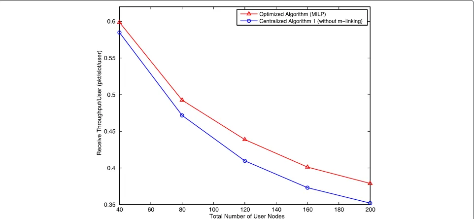
computational complexity, yields performance behavior that is only slightly degraded (around 10–15%) when compared with that exhibited by the MILP-based algo-rithm that yields the optimal schedule and transmit power

setting. It is noted that them-linkingprocess has not been invoked for this comparison.

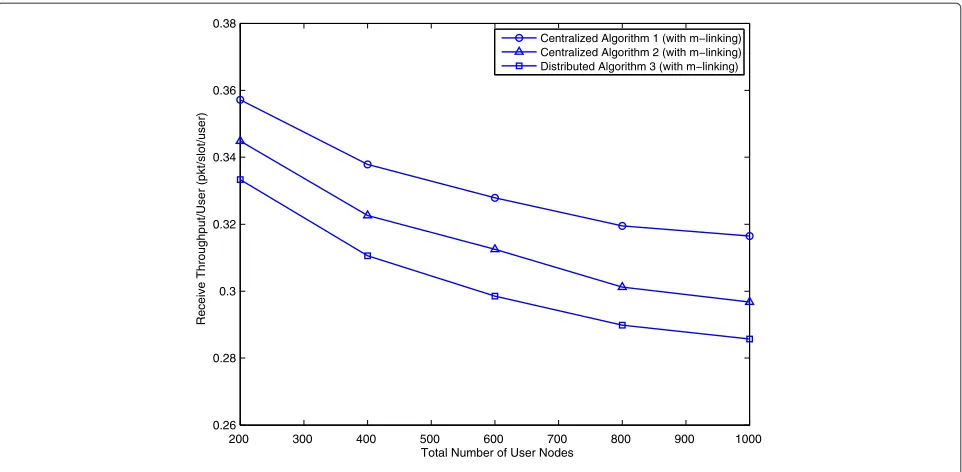
In Figure 4, we compare the per-user receive throughput rate, as a function of the total number of multicast clients

40 60 80 100 120 140 160 180 200

0.35 0.4 0.45 0.5 0.55 0.6

Total Number of User Nodes

Receive Throughput/User (pkt/slot/user)

Optimized Algorithm (MILP)

Centralized Algorithm 1 (without m−linking)

(12)

200 300 400 500 600 700 800 900 1000 0.26

0.28 0.3 0.32 0.34 0.36 0.38

Centralized Algorithm 1 (with m−linking) Centralized Algorithm 2 (with m−linking) Distributed Algorithm 3 (with m−linking)

Figure 4Performance comparison between the heuristic scheduling algorithms.

in the system, as attained by our algorithms. We observe that Algorithm 2 achieves a slightly lower throughput rate performance (by about 4–7%) than that attained under Algorithm 1, while Algorithm 3 exhibits a throughput rate that is further slightly degraded (by about 8–12%). We note that Algorithms 2 and 3 oﬀer much reduced level of algorithmic computational complexity, and that Algo-rithm 3 entails a fully distributed implementation. For all three algorithms, we observe that as the number of clients over a prescribed area of coverage increases, an increas-ing number of time slots per frame is required. However, the corresponding reduction in per-user throughput rate attained under each algorithm becomes much less notice-able with further increases in client population. The syn-thesized schedules tend to more fully cover the complete geographical area of operation, so that multicast schedules performed to accommodate a larger number of clients will then more often also cover new clients.

To assess the throughput gain attained by our adaptive power scheduling algorithms, when compared with LTE MBSFN schemes, we note the following. Assume that our multicasting scheme is used to share a prescribed LTE bandwidth segment, which consists of OFDM downlink channels, among neighboring base stations. Each sym-bol is transmitted across a narrow-band subcarrier, and is attached a cyclic preamble of sufficient length such that with the use of 1-tap equalization at the client receivers, no multipath fading interference is incurred [3]. Lognor-mal shadow fading effects can be readily included, but we neglect their effect in the following discussion since it does not impact our comparisons.

In assessing the performance behavior of OFDMA-based MBSFN systems, the study in [22] uses a bandwidth of 5 MHz and an ISD of 1.732 km. To attain complete coverage of all client nodes (at a BLER of 10%), it is deter-mined in [22] that the common MCS that must be used by all base stations corresponds to CQI 3, which maps to an SINR value of about −3 dB. The corresponding spectral efficiency is shown to be about 0.294 [bps/Hz]. Another MBSFN scheme presented in [5] assures a target coverage probability of 95%. Using an ISD of 1 km and a bandwidth of 5 MHz, it is shown that the best MCS to use for this ISD level is 16 QAM 1/2. Using this MCS, the system is shown to attain a spectral efficiency of about 0.28 [bps/Hz], and thus a throughput rate of about 1.4 Mbps for multicast-ing over a smulticast-ingle cell (see [5] Table III). In comparison, our “worst” performing Distributed Algorithm 3 achieves a throughput rate of about 0.28–0.33 [packets/slot/user], or 0.28ψ-0.33ψ[bps/Hz/user]. When the system operation is associated with an MCS code rate withψ= 2 [bps/Hz], such as 16 QAM 1/2, our scheme yields a throughput rate that is equal to about 0.56–0.66 [bps/Hz/user], leading to a data rate of 2.8–3.3 Mbps. This is higher than the spectral efficiency values of 0.28 and 0.294 [bps/Hz/user] achieved by [5,22], respectively.

(13)

the potential enhancement achievable with data rate adaptations. We further note that under our algorithms, neighboring base stations are not required to employ the same MCS. We conclude that our algorithms achieve performance eﬃciency that is as high as, or higher than, that attained by the referenced LTE MBSFN operations that employ sophisticated MIMO-type signal combining techniques.

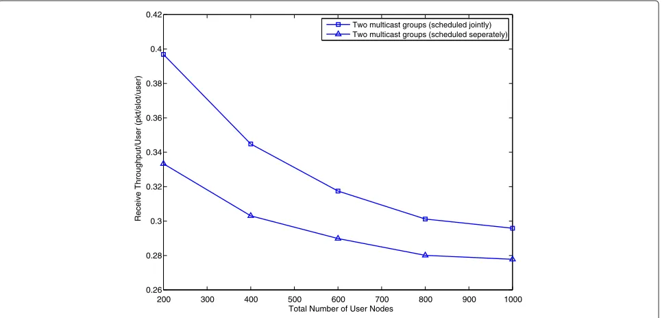
We next consider a system in which clients are divided into two multicast groups. We evaluate two multi-cast scheduling approaches. Under the ﬁrst approach, multicast transmissions to each group are separately scheduled—in each time frame, two sequential time-division subframes are executed, i.e., transmissions to group 1 clients are scheduled in subframe 1, followed by transmissions to group 2 clients in subframe 2. Such an operation mimics the MIMO approach, under which the same packets are scheduled for transmission at the same time by multiple base stations (though we employ no com-bining operations). In turn, under the second approach, multicast transmissions that belong to the two multicast group sessions are jointly scheduled. In this case, base stations that are scheduled to engage in transmissions in a certain time slot may use the allocated time slot to transmit packets that belong to any multicast group. For both cases, we have implemented the scheduling pro-cess by using Centralized Algorithm 2, incorporating the

m-linkingprocess. The performance results are displayed in Figure 5. They show that the joint scheduling scheme leads to a higher per-user throughput rate (by about 7– 16% for cases under evaluation). As noted above, the joint

scheduling operation provides much higher flexibility in accommodating transmissions of varying loading levels of multiple multicast group traffic flows. Such an operation is noted to lead to schedules that achieve higher spa-tial reuse factors, and therefore attain enhanced per-user throughput rate performance behavior.

To demonstrate the performance advantage that can be gained through the use of transmit power adaptations, we compare the performance of such adaptive-power algo-rithms with corresponding scheduling schemes that set the transmit power level of base stations to be fixed at their maximum specified levels. For both schemes, we uti-lize the scheduling mechanism specified by distributed heuristic Algorithm 3. Performance results are shown in Figure 6. We observe that by fixing the transmit power level, the scheduling scheme realizes a lower spatial reuse factor, requiring therefore a larger number of time slots to complete the execution of multicast transmissions, lead-ing to reduced per-user throughput rates by about 25–35% for the examined m-linking scenario. The results dis-played in Figure 6 also demonstrate the advantage gained through them-linking process; this process is noted to improve the throughput rate for the power adaptation scenario by about 11–16%.

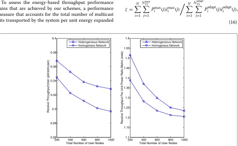
In Figure 7a, we compare the per-user throughput rate performance behavior attained under the homo-geneous and heterohomo-geneous layouts. We observe that our adaptive-power scheduling algorithms also oper-ate eﬀectively under a heterogeneous layout. Further-more, the latter layout is noted to lead to enhanced per-user receive throughput rates since our algorithms

200 300 400 500 600 700 800 900 1000

0.26 0.28 0.3 0.32 0.34 0.36 0.38 0.4 0.42

Two multicast groups (scheduled jointly) Two multicast groups (scheduled seperately)

(14)

200 300 400 500 600 700 800 900 1000

0.15 0.2 0.25 0.3 0.35 0.4

Distributed Alg. with Adaptive Power (with m−linking) Distributed Alg. with Adaptive Power (no m−linking) Distributed Alg. limited to use Max Power (with m−linking) Distributed Alg. limited to use Max Power (no m−linking)

Figure 6Performance comparison between adaptive-power scheduling algorithms and those that use ﬁxed base station transmit power levels.

eﬀectively use the micro base stations to cover their nearby clients. Under the homogeneous layout, the latter client nodes would reside in high interference cell-edge regions.

To assess the energy-based throughput performance gains that are achieved by our schemes, a performance measure that accounts for the total number of multicast bits transported by the system per unit energy expanded

is used. The ratio of the corresponding measures attained for the corresponding ﬁxed and adaptive power schemes, denoted asζis:

ζ = N

i=1 Nmax

TS

j=1

Pmax_i (j)I_imax(j)

N

i=1

N_TSadapt

j=1

P_iadapt(j)I_iadapt(j),

(16)

200 400 600 800 1000 0.26

0.28 0.3 0.32 0.34 0.36 0.38 0.4

Heterogeneous Network Homogeneos Network

200 400 600 800 1000 1.1

1.15 1.2 1.25 1.3 1.35 1.4 1.45 1.5 1.55 1.6

Receive Throughput Per Unit Power Ratio Metric (zeta)

Heterogeneous Network Homogeneos Network

(15)

where N_TSadapt and N_TSmax represent the number of time slots required by the employed adaptive and ﬁxed power schemes, respectively; Padapt_i (j) and Pmax_i (j) are the cor-responding transmit power levels selected for BS-iwhen scheduled to transmit its multicast messages in time slotj, and the indicator functionIi(j)is set to 1 if BS-iis assigned to transmit at time slotj, and is set to 0, otherwise. The sets {I_iadapt(j)} and {I_imax(j)} identify the schedule plans enacted under the adaptive and ﬁxed power schemes, respectively.

In computing the ratio metricζ involving the receive throughput rate per unit power, we observe in Figure 7b that the adaptive power scheme, when applied to the homogeneous base station layout, achieves a receive throughout rate per unit power performance that is about 20–38% higher than that obtained under the ﬁxed power scheduling scheme. An even better such energy aware performance metric is noted to be attained under the heterogeneous base station layout, yielding performance improvement factors of about 23–51% for the adaptive scheme. Thus, for the investigated simulation scenarios, the adaptive power scheduling scheme has been proven to derive schedules that yield high throughput rate and high throughput rate per unit power performance for homoge-neous as well as heterogehomoge-neous base station layouts.

Conclusions

In this article, we develop eﬃcient adaptive-power multi-cast scheduling algorithms for wireless cellular networks, under which base stations with multicast clients share their downlink channels, over an allocated frequency band on a spatial-TDMA basis. We model the schedul-ing problem as a MILP, which is NP-hard. Consequently, we present three heuristic algorithms of polynomial com-plexity for solving the problem in a practical manner. The algorithms make use of the coordinated operations among time-slot synchronized area base stations which jointly interact (through the use of a central controller, or in a distributed fashion) to determine their transmis-sion schedules and transmit power levels. Similarly, our adaptive-power scheduling algorithms lead to enhanced performance for mesh WiFi networks that use such coor-dinations among the system access points, or mobile back-bone based ad hoc wireless networks for which the elected backbone nodes employ such coordinated scheduling schemes. We show that further enhancement in through-put rate performance is achieved by using anm-linking

operation under which, when feasible, a client may be directed to receive multicast packets transmitted by a base station which is not the same one that it is associated with. For smaller systems, our simulation results demonstrate the performance of the system, when scheduling is per-formed by using our ﬁrst centralized heuristic algorithm,

to be in the 75 percentile of that exhibited by the opti-mal scheme. When considering larger network layouts, we show our heuristic adaptive-power scheduling algorithms to yield a per-user throughput rate that is higher than that attained by a fixed transmit power scheduling algorithm. Furthermore, our algorithms are shown to be more energy efficient than the corresponding fixed power schemes, on a throughput per unit consumed power basis. We also show that further enhancement in the throughput rate and throughput per unit power level is attained by using our adaptive-power scheduling algorithms in conjunc-tion with a heterogeneous network layout. In assessing the corresponding performance behavior exhibited by the illustrative LTE MBSFN multicast systems, we note our schemes to yield enhanced spectral efficiency levels when high user coverage is required, while involving much less restrictive synchronization mechanisms.

Competing interests

The authors declare that they have no competing interests.

Author details

1_{Electrical Engineering Department, University of California, Los Angeles, CA,}

USA.2_{Computer Science Department, Technion, Haifa, Israel.}

Received: 18 October 2011 Accepted: 11 July 2012 Published: 10 August 2012

References

1. 3GPP TS 23.246 v.10.2.0: Technical Speciﬁcation, Universal Mobile Telecommunications System, LTE, Multimedia Broadcast/Multicast Service, Architecture and Functional Description, Release 10, 2012 2. 3GPP TS 25.346 v.10.0.0: Technical Speciﬁcation, Universal Mobile

Telecommunications System, Introduction of the Multimedia

Broadcast/Multicast Service in the Radio Access Network, Release 10, 2011 3. F Khan,LTE for 4G Mobile Broadband(Cambridge University Press,

Cambridge, 2009)

4. A Alexiou, C Bouras, V Kokkinos, G Tsichrintzis, Communication cost analysis of, MBSFN in LTE. inProceedings of the IEEE 21st International Symposium on Personal Indoor and Mobile Radio Communications

(Istanbul, Turkey, 2010), pp. 1366–1371

5. L Rong, O Ben Haddada, SE Elayoubi, Analytical analysis of the coverage of a MBSFN OFDMA network. inProceedings of the IEEE Global Telecommunications Conference(New Orleans, LA, 2008), pp. 1–5 6. R Irmer, H Droste, P Marsch, M Grieger, G Fettweis, S Brueck, H Mayer, L

Thiele, V Jungnickel, Coordinated multipoint: concepts, performance, and ﬁeld trial results. IEEE Commun. Mag.49(2), 102–111 (2011)

7. P Marsch, G Fettweis, On multi-cell cooperative transmission in backhaul-constrained cellular systems. Ann. Telecommun.63(5), 253–269 (2008)

8. R Cruz, A Santhanam, Optimal routing, link scheduling and power control in multi-hop wireless networks. inProceeding of the IEEE International Conference on Computer Communications(San Francisco, CA, 2003), pp. 702–711

9. A Behzad, I Rubin, Optimum integrated link scheduling and power control for multihop wireless network. IEEE Trans. Veh. Technol.56(1), 194–205 (2007)

10. A Behzad, I Rubin, J Hsu, On the performance of the randomized power control algorithms for random multiple access in wireless networks. in

Proceedings of the IEEE Wireless Communications and Networking Conference(New Orleans, LA, 2005), pp. 707–711

11. W Liang, Approximate minimum-energy multicasting in wireless ad hoc networks. IEEE Trans. Mobile Comput.5(4), 377–387 (2006)

(16)

Proceeding of the IEEE International Conference on Computer Communications(Tel-Aviv, Isreal, 2000), pp. 585–594

13. 3GPP TS 25.214 v.10.5.0: Technical Speciﬁcation, Universal Mobile Telecommunications System, Physical Layer Procedures, Release 10, 2012 14. A Behzad, I Rubin, High transmission power increases the capacity of ad

hoc wireless networks. IEEE Trans. Wirel. Communi.5(1), 156–165 (2006) 15. T Rappaport,Wireless Communications: Principles and Practice,2nd edn.

(Prentice-Hall, Englewood Cliﬀ, NJ, 2002)

16. B Noble, J Daniel,Appied Linear Algebra,3rd edn. (Prentice-Hall, Englewood Cliﬀ, NJ, 1988)

17. N Bambos, S Chen, G Pottie, Radio link admission algorithms for wireless networks with power cotnrol and active link quality protoction. in

Proceeding of the IEEE International Conference on Computer Communications(Boston, MA, 1995), pp. 97–104

18. M Pursley, H Russell, J Wysocarski, Energy-eﬃcient transmission and routing protocols for wireless multiple-hop networks and

spread-spectrum radios. inProceeding of the IEEE/AFCEA EUROCOMM 2000, Information Systems for Enhanced Public Safety and Security(2000), pp. 1–5 19. M Halldorsson, J Radhakrishnan, Greed is good: approximating

independent sets in sparse and bounded-degree graphs. Algorithmica. 18(1), 145–163 (1997)

20. T Lee, J Lin, Y Su, Downlink power control algorithms for cellular radio systems. IEEE Trans. Veh. Technol.44(1), 89–94 (1995)

21. V Abhayawardhana, I Wassell, D Crosby, M Sellars, M Brown, Comparison of empirical propagation path loss models for ﬁxed wireless access systems. inProceedings of the IEEE Vehecular Technology Conference

(Stockholm, Sweden, 2005), pp. 73–77

22. A Alexiou, C Bouras, V Kokkinos, G Tsichritzis, Spectral eﬃciency performance of MBSFN-based LTE networks. inProceedings of the IEEE International Conference on Wireless and Mobile Computing, Networking and Communications(Chengdu, China, 2010), pp. 361–367

doi:10.1186/1687-1499-2012-250

Cite this article as:Rubinet al.:Joint scheduling and power control for multicasting in cellular wireless networks.EURASIP Journal on Wireless

Com-munications and Networking20122012:250.

Submit your manuscript to a

journal and beneﬁ t from:

7Convenient online submission

7Rigorous peer review

7Immediate publication on acceptance

7Open access: articles freely available online

7High visibility within the ﬁ eld

7Retaining the copyright to your article

References

1. 3GPP TS 23.246 v.10.2.0: Technical Specification, Universal Mobile Telecommunications System, LTE, Multimedia Broadcast/Multicast Service, Architecture and Functional Description, Release 10, 2012 2. 3GPP TS 25.346 v.10.0.0: Technical Specification, Universal Mobile