Time Domain Sparse Representation for Multi-Aspect SAR Data of Targets

(1)

Time Domain Sparse Representation for Multi-Aspect

SAR Data of Targets

Jinrong Zhong*, Gongjian Wen, Conghui Ma, and Baiyuan Ding

Abstract—Sparse representation is the fundamental technology of compressive sensing, sparse three-dimensional (3-D) imaging, and dictionary-based parameter estimation. Typical sparse representation models of radar signal work in the frequency domain, which may encounter high dimension and large data amount of dictionary. This paper presents a time-domain (TD) representation model for multi-aspect SAR data. We generate the multi-aspect two-dimensional (2-D) TD responses of the 3-D scattering center model. Then we cut off the low-energy area of the 2-D TD response and use cutoff responses to construct the dictionary of sparse representation. Such a TD dictionary is a sparse matrix. Moreover, we build and solve the sparse representation model based on the TD dictionary. Compared with the frequency-domain (FD) sparse representation model, the data size of our TD dictionary is remarkably lower, and the solving of TD sparse representation problem is in higher efficiency. We utilize the TD sparse representation to reconstruct 3-D images from multi-aspect SAR data. Experimental results demonstrate the effectiveness and efficiency of the TD sparse representation model.

1. INTRODUCTION

Sparse representation of radar signals [1] is the fundamental for many other techniques, such as compressed sensing [2], sparse 3-D imaging [3], data compression [4], and dictionary-based parameter estimation [5]. Multi-aspect SAR data are a typical collecting geometry of radar [6]. Sparse representation of multi-aspect SAR data is of signiﬁcance.

The existing sparse representation models [1–5] for radar signal are established in the frequency domain. In other words, these sparse representation methods built the dictionary and solved the model in the frequency domain. Based on frequency-domain (FD) sparse representation model, many achievements [1–5, 7, 8] have been made in the ﬁles of 3-D imaging and feature extraction. However, the larger data amount of the dictionary, accompanied with a huge computation, is always a signiﬁcant challenge.

For the sparse representation problem of multi-aspect SAR data, this paper proposes a time-domain (TD) model, which constructs the dictionary in the time domain and solves the sparse representation problem in time domain too. We use 2-D time responses of the 3-D scattering center model at every aspect to construct the dictionary. Since the energy of 2-D TD responses concentrates on several small regions, we cut off the low-energy areas to make the TD dictionary become a sparse matrix. Moreover, the signal to noise rate (SNR) of the valid regions increases in the time domain. So the time domain sparse representation reduces the data amount of dictionaries substantially and improves the searching efficiency. Apply the proposed TD sparse representation to the multi-aspect SAR data of 3-D imaging. The experimental results demonstrate that TD sparse representation is effective and exhibit its efficiency.

Received 24 April 2015, Accepted 14 July 2015, Scheduled 14 August 2015

* Corresponding author: Jinrong Zhong ([email protected]).

(2)

Sensor

Xground

Yground Zground

wz

wy

wx

Dk

~

D~₁

(a) (b)

Figure 1. Multiple-aspect SAR collecting geometry. (a) Collecting geometry. (b) Fractions in wavenumber coordinate system.

2. MULTI-ASPECT COLLATED SAR DATA

The multi-aspect collected geometry is depicted in Figure 1. At the observed angle (φ, θ), the radar received signal is r(t;θ, φ) = [_Λg(x, y, z;θ, φ)dxdydz]∗ s(t), and s(t) is the sent signal, ∗ the convolution. Using the signal model presented by Austin et al. in [3], interpret multi-aspect SAR data in the 3-D Fourier transformationG(w_x, w_y, w_z) of the reﬂectivity functiong(x, y, z;φ, θ). As can be seen below, our method does nothing matter with the polarization, and we take single polarization in consideration only. The signal model in Fourier transformation is given by

G(w_x, w_y, w_z) =

N

n=1

g(x, y, z;φ, θ)·e−j(xnwx+ynwy+znwz) (1)

Suppose that the center frequency of k-th aspect is f_c,k, the bandwidth B_k, and the aperture ¯

φ_k, k = 1, . . . , K. By the projection-slice theorem, each aperture is a fraction in G(w_x, w_y, w_z). Denote thek-th fraction’s sample point set asM_k={(f_j, φ_i)}Nfk,Mfk

j=1,i=1 . The coordinates in wavenumber domain are w_xj,i,k = −4πf_jcosθ_i,kcosφ_i,k/c, wj,i,k_y = −4πf_jcosθ_i,ksinφ_i,k/c, w_zj,i,k = −4πf_jsinθ_i,k/c. Reshape them into a vector H_M =∪K_k₌₁H_M,k={_m}M_m₌₁,M =K_k₌₁M_k, and them-th coordinate is m= (wx,m, wy,m, wz,m).

Denote the multi-aspect SAR dataset as ˜D={D˜_k}K_k₌₁, and ˜D_k = [G(w_xj,i,k, wj,i,k_y , wj,i,k_z )]Mfk,Nfk i=1,j=1 is thekaspect fraction. Transform ˜D_k into a 2-D SAR complex image and denote it asD_k∈CM zk×N zk, which can be viewed as 2-D time domain data. M z_k and N z_k are the row and column numbers.

3. FREQUENCY DOMAIN SPARSE REPRESENTATION

Sample 3-D imaging spaceQ into a series of 3-D locations as candidate locations,

Q_M ={λ¯1, . . . ,λ¯N}={(xn, yn, zn)}Nn=1 (2)

UsuallyQ_M is chosen on a uniform rectilinear grid. The grid point number isN. Take the isotropic point scattering center (IPS) model to construct the dictionary and sparse representative the target. The dictionary is built in the frequency domain, using the FD responses of IPS

˜

Y=F(H_M,Q_M) =

e−j(xnwx,m+ynwy,m+znwz,m)

m,n (3)

where m indexes the M measured frequency (or wavenumber) domain down rows, and n indexes the location across columns. Based on ˜Y, the vectored measured data can be approximated as

˜

(3)

where ˜d ∈ CM×1 is vectored from the multi-aspect SAR data, and ˜v is the noise. s is a sparse N -dimensional vector and also the scattering amplitude vector. ˆsis the solution of the sparse optimization problem

ˆs= arg mins₀ s.t. Ys˜ −d

2 < ε (5)

4. TIME DOMAIN SPARSE REPRESENTATION

The 3-D scattering center models have a natural characteristic: the amplitudes of its 2-D response at every aspect are well distributed in the frequency domain while the amplitudes are uneven in the time domain. We develop a TD sparse representation model, exploiting such a property.

As presented above, for a location ¯λ_n= [x_n, y_n, z_n]T inQ_M, the 2-D FD response at thekaspect is

˜

E(H_M,k|λ¯_n) =

exp

−j

x_nw_x,ki,j +y_nwi,j_y,k+z_nwi,j_z,k Mfk,Nfk

i=1,j=1 (6)

˜

E_k,n = ˜E(H_M,k|λ¯_n) is aMf_k×Nf_k matrix. Interpolate and transform ˜E_n to the time domain

E_k,n=F₂−1·B·E˜_k,n (7)

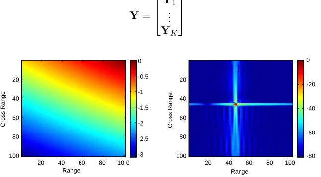
Here,F₂−1(·) represents the 2-D inverse fast Fourier transform (IFFT), andBrepresents interpolate the 2-D sector data into rectangular data. Figure 2 shows an example of the 2-D frequency/time domain responses at the k aspect. It can be found that the energy of TD response, E_k,n = [e_i,j,k]M zk_i₌₁_,j×₌₁N zk, concentrates in a small region. The other big region is lower than −50 dB of the peak-power. This characteristic does not depend on the measurement data, but a natural characteristic scattering center model. We cut oﬀ the small amplitude regions

e_i,j,k =

0 |e_i,j,k|< ξ_n

e_i,j,k else (8)

Here, ξ_n is an adaptive threshold. Its value is determined by equation ξ_n = max(|E_k,n|)·10βd/20_. max(|E_k,n|) is the maximum amplitude of E_k,n. β_d(β_d < 0) is an experiential threshold for the whole dictionary. Write such processing in the form of an operator, E∗_k,n = Γβd(E_k,n). We stack the cutoﬀ 2-D response E∗_k,n into a vector denote as ψ_k,n = vec(E_k,n∗ ) = [ϕ1,n, . . . , ϕMk,n]T. It is the

component of ¯λ_n at the k-th aspect. We express the process of getting ψ_k,n in the form of operators, ψk,n = vec·Γβd·F2−1·B·E˜k,n. Thekpart of the TD dictionary,Yk, consists of all theψk,n atkaspects

for all ¯λ_n, n = 1, . . . , N. After obtaining all the K parts, we construct the dictionary of Q_M for the multi-aspect SAR data as

Y=

⎡ ⎣

Y1 .. .

Y_K

⎤

⎦ (9)

Range

Cross Range

20 40 60 80 10 0 20

40

60

80

100 -3

-2.5 -2 -1.5 -1 -0.5 0

Range

Cross Range

20 40 60 80 100 20

40

60

80

100 -80

-60 -40 -20 0

(4)

When β_d > −∞, Y is a sparse 2-D matrix. Suppose that Q is the number of nonzero elements and that η = Q/(M ·N) is the proportion of nonzero elements and indicates the sparse degree of the dictionary matrix. The largerβ_dis, the smallerηis, and the sparser isY, which is beneﬁcial to reducing the data size of dictionaries. In addition, Y being a sparse matrix, is beneﬁcial to reducing the burden of computation.

Interpolate and transform ˜D_k to the time domain, and then stack it into aM_k-dimensional vector

d_k = [d, . . . , d_m, . . . , d_Mk]T = vec·F₂−1·B·D˜_k. So, the measured data can be approximated as

d=Ys+v, here, d=

⎡ ⎣

d1 .. .

d_Nap

⎤

⎦ (10)

wherevis TD noise vector,sa sparse vector, anddthe vectored multi-aspect SAR TD data. According to the time-frequency duality principle, as β_d = −∞ (in other words, the time-domain dictionary is not cut off), the FD model (4) and TD model (10) are equivalent. Also, their solutions should be the same. As β_d≥ −∞, due to truncation processing, which make the dictionary loss energy and rice the atomic correlation, the solutions of the model (4) and model (10) may be different. But it cannot assert that the convergence and accuracy of model (10) is inferior to model (4). Because the energy of target responses congregates in TD, the SNR rises in the active area. And the truncation not only cut off signals in the dictionary, but also cut off the noise in the measurement data covertly. These factors are conducive to the solution. Solve the sparse optimization problem to obtain ˆs∗,

ˆ

s∗ = arg mins₀ s.t. Ys−d2₂< ε (11)

Since l0-regulated optimization is hard to solve, we take thel1-regulated technique [9, 11] to deal with problem (11)

ˆs∗ = arg min

Ys−d2₂+λs₁

(12)

5. EXPERIMENTAL RESULTS

We use the TD sparse model to representative multi-aspect SAR data simulated by GTD [10] model, then compare the performances of TD model with the FD model. The performances include validity and eﬃciency. In order to demonstrate the validity of the TD sparse representation, we compare the sparse solutions, scattering center locations and the reconstructed 2-D SAR images with the FD method. In order to demonstrate the eﬃciency, we compare their dictionaries’ data size and time consumption of solving.

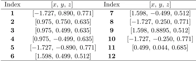
The simulated complex target consists of 11 scattering centers, which are located in range

Q = {x, y, z| −2 < x < 2,−2 < y < 2,0 < z < 1}. The locations of them are listed in Table 1. Use GTD-based scattering center model [10] to produce multiple-aspect SAR data

G(w_x, w_y, w_z) =

P

i=1

A_i·(jf /f_c)αi·e−j(xiwx+yiwy+ziwz)+v

Table 1. The locations of target’s 11 scattering centers.

Index [x, y, z] Index [x, y, z]

1 [−1.727, 0.890, 0.771] 7 [1.598, −0.499, 0.512]

2 [0.975, 0.750, 0.635] 8 [−1.727, 0.250, 0.771]

3 [0.975, 0.499, 0.635] 9 [1.598, 0.8895, 0.512]

4 [0.975, −0.499, 0.635] 10 [−1.727, −0.250, 0.771]

5 [−1.727,−0.890, 0.771] 11 [0.499, 0.044, 0.685]

(5)

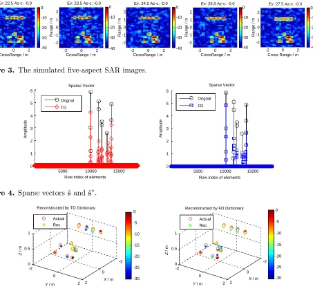
A_i is randomly generated, and frequency-dependent factor α_i is set to one of [−1,−1/2,0,1/2,1] randomly. Produce SAR data at ﬁve aspects (θ_k, φ_k). The azimuths are φ_k = 5◦, k = 1, . . . ,5, and the elevations areθ1 = 22.5◦,θ2 = 23.5◦,θ3 = 24.5◦,θ4 = 25.5◦,θ5 = 27.5◦. The sample intervals are Δf = 30 MHz and Δφ= 0.1◦. Add zero-mean white Gaussian noise v∼N(0, σ2

v) to make the FD

SNR_{F d} =−10 dB, TD SNRimg = 20 dB. The ﬁve SAR images with noise are shown in Figure 3, and

the dynamic range for display are [−40, 0] dB.

Take intervals Δx = 0.1 m, Δy = 0.1 m, Δz = 0.1 m to grid the 3-D space Q into a set of 3-D locations,N = 18491 locations in total. So, the sparse dictionaries’ demotion isM×N = 4420×18491. Construct the TD dictionary with a threshold β_d = −50 dB. The proportion of nonzero elements is

η = 7.1%. It is lower than a FD dictionary in an order of magnitude. Solve the sparse representation problem ˜d = ˜Y·s+ ˜v and d =Y·s+v. The sparse vectorsˆs and ˆs∗ are shown in Figure 4. Their corresponding locations are shown in Figure 5. As an example, we use ˆs∗ to reconstruct the SAR image at (θ1 = 25.5◦, φk = 5◦) by Y·ˆs∗ directly, then use ˆs to rebuild the FD SAR data and turn it into

image-domain. The reconstructed images are shown in Figure 6.

From Figure 4, it can be seen that ˆs∗is convergent to the real sparse vector. There is little diﬀerence between sparse vectors ˆsand ˆs∗. Figure 5 conﬁrms such a judgment. Since the scattering centers are not

-2 0 2 -2

-1 0 1 2

CrossRange / m

Range / m

Ev: 22.5 Az-c: -0.0

-40 -30 -20 -10 0

-2 0 2 -2

-1 0 1 2

CrossRange / m

Range / m

Ev: 23.5 Az-c: -0.0

-40 -30 -20 -10 0

-2 0 2 -2

-1 0 1 2

CrossRange / m

Range / m

Ev: 24.5 Az-c: -0.0

-40 -30 -20 -10 0

-2 0 2 -2

-1 0 1 2

CrossRange / m

Range / m

Ev: 25.5 Az-c: -0.0

-40 -30 -20 -10 0

-2 0 2 -2

-1 0 1 2

Cross Range / m

Range / m

Ev: 27.5 Az-c: -0.0

-40 -30 -20 -10 0

Figure 3. The simulated ﬁve-aspect SAR images.

5000 10000 15000 0 1 2 3 4 5 6 Sparse Vector

Row index of elements

Amplitude

Orignal

TD

5000 10000 15000 0 1 2 3 4 5 6 Sparse Vector

Row index of elements

Amplitude

Orignal

FD

Figure 4. Sparse vectors ˆs and ˆs∗.

-2 0 2 -2 0 2 0 0.5 1

X / m

Reconstructed by TD Dictionary

Y / m

Z / m -30 -25 -20 -15 -10 -5 0 Actual Rec -2 0 2 -2 0 2 0 0.5 1

X / m

Reconstructed by FD Dictionary

Y / m

Z / m -30 -25 -20 -15 -10 -5 0 Actual Rec

(6)

-2 -1 0 1 2 -2

-1 0 1 2

Reconstructed by TD-S Ev: 25.5

Cross Range / m

Range / m

-40 -30 -20 -10 0

-2 -1 0 1 2

Reconstructed by FD-S Ev: 25.5

Cross Range / m

Range / m

-40 -30 -20 -10 0

Figure 6. The reconstructed SAR images.

right on the grid, the nonzero elements are located around the real scattering centers. The color is the value of the nonzero elements, also is the amplitude locations. They are can be viewed as 3-D images of the simulated target. We can see that the two almost identical images are reasonable. Both the TD and FD dictionary sparse representations can availably represent the target. In Figure 6, the reconstructed SAR images are with less noise. The ﬁrst one is reconstructed by TD sparse representation, and it is 0.958 similar to the original noise-free SAR complex image. The second one is reconstructed by FD sparse representation, and its similarity is 0.958. The formula to calculate the similarity is

μ= (ˆe−e)H ·(ˆe−e)/eH ·e

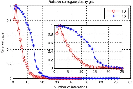
From the results presented above, it can be said that the TD sparse representation is eﬃcacious. Below, we discuss the eﬃciency. First, as mentioned above, compared with the FD dictionary, the data size of our TD dictionary reduces 92.9%. Second, we examine the computation complexity of solving our sparse representation problem, in comparison with the FD one. In this experiment, we use the method proposed by Kim et al. for l1-regularized least squares in [11] to solve the TD and FD sparse representation problems. The corresponding l1 ls Matlab solver is presented in [12]. The TD

(7)

0 10 20 30 40 50 60 70 80 0

0.2 0.4 0.6 0.8 1

Relative surrogate duality gap

Number of interations

Relative gaps

TD FD

0 5 10 15 20 25 0

0.2 0.4 0.6 0.8 1

Figure 7. The relative surrogate duality gaps of TD method and FD method.

but also the iteration number decreases. We plot the relative surrogate duality gaps of TD method and FD method again in Figure 7 with an enlarged subplot. It suggest that the cost function is smoothed. Furthermore, we try to explain the mechanism in detail by theoretical analysis. Suppose that ˜Y is the FD dictionary. As d=e+v, the searching for the minimum will be interfered noise v.

Δ(s) =d−Ys˜

2

2+λ||s||1

We index the iteration times withitand suppose that the desired search direction at current point

s_it is∇0_it

Δ0

s_it+∇0_it =e−Y˜

s_it+∇0_it 2 2+λ

s_it+∇0_it 1

Due to the noise, there may be another disturbance direction ∇∗_it that makes Δ(s_it +∇∗_it) ≤ Δ(s_it + ∇0_it). This is probabilistic. The larger is the noise, the greater is the probability. In our TD model, we transform ˜Y into TD ﬁrst. Y∗ is the un-cutoﬀ time-domain dictionary and Δ(s_it) = ||d −Y∗s_it||2₂ +λ||s_it||1. Suppose that [Y∗sit]Lit is the low energy area of Y∗sit, in which

the elements will be set to zero. [Y∗s_it]Γ_it is the high energy area, in which the elements maintain the original values. [·]L_it∩[·]Γ_it =∅. We rewrite Δ1(sit) =||d−Y∗sit||22 as,

Δ1=d−Y∗sit22 =[d]Lit+ [dit]Γit−[Y∗sit]Lit−[Y∗sit]Γit₂

=[d]L_it−[Y∗s_it]L_it2 2+

[d]Γ_it−[Y∗s_it]Γ_it2 2+ 2

[d]L_it−[Y∗s_it]L_it H

[d]Γ_it−[Y∗s_it]Γ_it

Here, [·]L_it and [·]Γ_it are determinate according toY∗s_it adaptively. [d]L_it represents that the elements ind

corresponding to the low-energy area [·]L_it remain, and the rest are set to zero. [d]Γ_it represents that the elements in d corresponding to the area [·]Γ_it. Since [·]_itL∩[·]Γ_it =∅, ([d]0_it−[Ys]0_it)H([d]Γ_it−[Ys]Γ_it) = 0, so Δ1(sit) =||[d]itL−[Y∗sit]Lit||22+||[d]Γit−[Y∗sit]Γit||22. Then,

Δ(s_it) =[d]L_it−[Y∗s_it]L_it2₂+[d]Γ_it−[Y∗s_it]Γ_it2₂+λs_it₁

The SNR of [d]Γ_it is higher than the SNR of [d]L_it, and the convergence of||[d]Γ_it−[Y∗s_it]Γ_it||2₂ should be better than |[d]L_it−[Y∗s_it]L_it||2₂. In our TD method, we set [Ys]L_it =0. [·]L_it can also be expressed as [·]0_it.

Δ(s_it) =[d]_it02₂+[d]_itΓ −[Y∗s_it]Γ_it2₂+λs_it₁

If [·]0_it₊₁ is not changed, ||[d]0_it||2₂ =|[d]0_it₊₁||2₂ is a constant, which will not aﬀect the searching of descent direction. If [·]0_it₊₁ is changed, for a right descent direction ∇_it, |[d]0_it||2₂ ≤ [d]0_it₊₁||2₂ must be true. The convergence of||[d]0_it||2

(8)

the real solution s, it is important and benefitial to the convergence of Δ(s). Of course, when s_it has been very close to the real solutions, the convergence speed of||[d]Γ_it−[Y∗s_it]Γ_it||2₂will be slower than the original||d−Y∗s_it||2₂. Because at such case, ||[d]0_it−[Y∗s_it]0_it||2₂ will also converge to a minimum s. In other words, the descent directions of||[d]0_it−[Y∗s_it]0_it||2₂ and||[d]Γ_it−[Y∗s_it]Γ_it||2₂ may be the same with great probability, and||[d]0_it₊₁−[Y∗s_it+1]0_it₊₁||2₂≤ |[d]0_it|2₂. So, it can be forecasted that the convergence speed of our TD model is slower than the FD one whens_itis close tossince some signal is lost as we set [Y∗s_it]0_it=0. However, at the beginning of the iteration,s_itis far froms, and the convergence speed of our TD model is faster. The descent directions keep the same as the noiseless case||e−Ys˜ _it||2₂+λ||s_it||1 with great probability when the effect of most of the noise is dispelled. As a comprehensive effect, the convergence speed and time consumption of our TD model are superior to the FD one, which has been exhibited in our experiment. When β_d =−∞, there is no truncation, but a large number of elements in the TD dictionary approach zero. Therefore, the TD sparse representation also has such a character.

6. CONCLUSIONS

This paper proposes a concept of TD sparse representation for multi-aspect SAR data and presents the method of constructing TD dictionary and solving TD sparse representation problem. Compared with the FD model, the data size of the TD dictionary consisting of truncated 2-D TD responses is far smaller. And it improves the convergence speed of the optimization algorithm. Experimental results show that the TD sparse representation is available, and its eﬀectiveness is considerably advanced.

REFERENCES

1. Samadi, S., M. C¸ etin, and M. A. Masnadi-Shirazi, “Sparse representation-based synthetic aperture radar imaging,”IET Radar, Sonar, Nav., Vol. 5, No. 2, 182–193, 2011.

2. Herman, M. A. and T. Strohmer, “High-resolution radar via compressed sensing,” IEEE Trans. Signal Process., Vol. 57, No. 6, 2275–2284, 2009.

3. Austin, C. D., E. Ertin, and R. L. Moses, “Sparse signal methods for 3D radar imaging,” IEEE Journal of Selected Topics in Signal Processing, Vol. 5, No. 3, 408–423, 2011.

4. Bhattacharya, S., T. R. Blumensath, B. Mulgrew, and M. Davies, “Synthetic aperture radar raw data encoding using compressed sensing,” Proc. IEEE 2008 Int. Conf. Radar, 1–5, 2008.

5. Austin, C. D., J. N. Ash, and R. L. Moses, “Dynamic dictionary algorithms for model order and parameter estimation,” IEEE Trans. Signal Process., Vol. 61, No. 20, 5117–5130, 2013.

6. Rigling, B. D. and R. L. Moses, “Three-dimensional surface reconstruction from multi-static SAR images,”IEEE Trans. Image Process., Vol. 14, No. 8, 1159–1171, 2003.

7. Corporation, H. P., “Sparse representation denoising for radar high-resolution range proﬁling,”Int. J. Antennas Propagat., Vol. 13, No. 1, 479–482, 2014.

8. Zhu, S., A. Mohammad-Djafari, H. Wang, B. Deng, L. Xiang, and J. Mao, “Parameter estimation for SAR micromotion target based on sparse signal representation,”EURASIP J. Advances Signal Process., Vol. 13, No. 2, 26–26, 2012.

9. Zhu, X. X. and R. Bamler, “Tomographic SAR inversion by L1-norm regularization: The compressive sensing approach,” IEEE Trans. Geosci. Remote Sens., Vol. 48, No. 10, 3839–3846, 2010.

10. Potter, L. C., D. M. Chiang, R. Carriere, and J. Gerry, “A GTD-based parametric model for radar scattering,”IEEE Trans. Antennas Propagat., Vol. 43, No. 11, 1058–1067, 1995.