High Speed Model Implementation and Inversion Techniques for Smart Material Transducers

(1)

BRAUN, THOMAS R. High Speed Model Implementation and Inversion Techniques for Smart Material Transducers. (Under the direction of Professor Ralph C. Smith).

(2)

TECHNIQUES FOR SMART MATERIAL TRANSDUCERS

by

Thomas R. Braun

A dissertation submitted to the Graduate Faculty of North Carolina State University

in partial fulfillment of the requirements for the Degree of

Doctor of Philosophy

APPLIED MATHEMATICS

Raleigh, North Carolina 2007

APPROVED BY:

Ralph C. Smith Hien Tran

Chair of Advisory Committee

(3)

DEDICATION

(4)

BIOGRAPHY

Thomas R. Braun received his Bachelor’s degree in applied mathematics from Asbury College in May 2001. Although originally planning on continuing straight to graduate school, an offer from Los Alamos National Laboratory (LANL) convinced him to take some time away from formal studies. Tom spent three years in the space engineering group at LANL, working on signal processing algorithms for remote sensing. During this time, he met his wife Sarah at a Bible study, and they were married on August 2, 2003. The two left Los Alamos in the summer of 2004 to continue studies, Tom in applied mathematics at North Carolina State, and Sarah in elementary education at Campbell. On January 12, 2006, Tom and Sarah welcomed a new family member with the birth of their son, Matthew Ryan Braun.

(5)

ACKNOWLEDGEMENTS

I would like to thank Professor Ralph Smith for his support and advice throughout this entire process, starting even before I arrived at North Carolina State as a student. His advice, direction, and support has been and continues to be invaluable. I’d also like to thank Professors Hien Tran, Pierre Gremaud, and Stefan Seelecke for their help and support on my committee, and all of my professors and fellow graduate students. The community here as a whole have made this a very friendly, welcoming place to learn and work.

(6)

List of Figures

Figure 1.1 Diagram of the lattice structure of the piezoceramic PbTiO3. . . 3

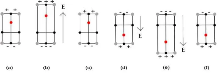
Figure 1.2 PZT data from [51] illustrating time-dependent material properties. (a) Nonclosure of field-polarization minor loops, and (b), (c) change in polar-ization for fixed input field values. . . 5 Figure 1.3 Magnetic field versus magnetization for a steel rod. Data taken from [5]. 5 Figure 1.4 Representation of phases exhibited by shape memory alloy crystals, (a)

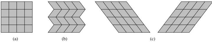
the high-symmetry austenite phase, (b) martensite phases in the twinned configuration which preserves the same macroscopic shape as the austenite configuration possessed, and (c) detwinned martensite variants in which a macroscopic strain is manifested. . . 6 Figure 1.5 Response of the shape memory alloy NiTi. (a) Stress versus strain

un-der moun-derately fast loading [28] and (b) temperature versus strain for a constant load [17]. . . 7 Figure 2.1 Helmholtz energy function (2.5). . . 9 Figure 2.2 Comparison of model versus data for a cylindrical steel rod [5]. (a) shows

the input field used in (b) and (c), which gives a sequence of three minor loops. (c) is a close-up of (b). The magnetic field seen in (d) gives the magnetization shown in (e) and (f). The field is held constant from the point delineated by the vertical black line. It is noted that the magneti-zation continues to creep up after this point. . . 12 Figure 2.3 Comparison of model versus data for (a) PLZT and (b) Terfenol-D. PLZT

data is taken from [20] whereas Terfenol-D data is courtesy of Marcelo Dapino at The Ohio State University. . . 13 Figure 2.4 Comparison between the backward Euler approximation (2.22) and

ana-lytic approximation (2.23) for an example input, with parameters taken to match PLZT. (a) Entire hysteresis curve, and (b) magnified view. . . . 15 Figure 2.5 Plot ofM(H;x+) for 6 intervals of composite 4-point Gaussian quadrature

(9)

Figure 2.6 Comparison of M(H;x+) for 6 intervals of composite 4-point Gaussian

quadrature on each distribution. . . 17 Figure 2.7 Prototypical rod used to construct overall model. . . 22 Figure 3.1 Control configuration utilizing an inverse model and a linear control law. 25 Figure 3.2 (a) Reference polarization and (b) electric field E given by the inverse

model with parameters estimated for PLZT. (c) Comparison of the re-sulting polarization P and the reference polarization Pb. (d) Absolute error_|Pb₋P_|. . . 28 Figure 3.3 (a) Reference polarization and (b) electric field E given by the inverse

model with parameters estimated for PLZT. . . 29 Figure 3.4 (a) Reference magnetization and (b) magnetic fieldHgiven by the inverse

model with parameters estimated for Terfenol-D. . . 30 Figure 3.5 Results for the combined inverse model with parameters estimated for

a Terfenol-D rod. (a) Specified displacement u_b and (b) magnetic field

H provided by the inverse algorithms. (c) Absolute error _|bu₋ u_| for displacement ugiven by the rod model. . . 31 Figure 4.1 Possible polarization states of a single crystal including (a) the state with

no applied field, (b) the 180◦ _{switch which occurs with a sufficiently strong}

negative field, and (c) a 90◦ _{switch induced by stress. . . .} ₃₂

Figure 4.2 PLZT data showing the effect of stress on polarization [20]. . . 33 Figure 4.3 Comparison of E ₋P curves from the negligible relaxation model with

PLZT data from [20] for compressive prestresses of (a) σ0 = 0 MPa, (b) σ0 =−6 MPa, (c) σ0 =−10 MPa and (d)σ0 =−15 MPa. . . 37

Figure 4.4 Comparisons of the (a) polarization and (b) error in polarization given by a direct implementation of the stress-dependent, negligible relaxation model and an implementation based on look-up tables (LUT) with and without interpolating between the table elements. . . 39 Figure 4.5 Comparisons of the polarization given by a direct implementation of the

stress-dependent relaxation model and an implementation based on look-up tables. . . 41 Figure 4.6 Results of the inverse model for the input polarization (a) and stress (b)

with ∆t= 1_×10−4_{. The resulting electric field and error in polarization for}

(10)

Figure 5.1 Helmholtz energies in shape memory alloys for (a) temperatures where the austenite phase is stable and (b) temperatures where only martensite is stable. . . 48 Figure 5.2 (b) Comparison of SMA model response to stress-strain data [28] for the

applied stress given in (a) and a constant ambient temperature of 293 K. (c) Internal temperature (spatial average) predicted by the model. . . 54 Figure 5.3 Comparison of SMA model response to temperature-strain data [17] for

the dynamic external temperature given in (a) and a constant applied stress of 200 MPa. The internal temperature (spatially averaged) of the material predicted by the model is also given in (a), while both the mea-sured and predicted strain are given in (b). . . 55 Figure 5.4 Pseudocode to update the phase fractions for regimes where austenite is

stable using the pseudoanalytic method. . . 59 Figure 5.5 Applied stress employed for the results in Figure 5.6 and Tables 5.1 and

5.2. . . 61 Figure 5.6 Comparison of the model results for the (a), (c), and (e) backward Euler

algorithm and (b), (d), and (f) pseudoanalytic method for the stress input given in Figure 5.5. (a) and (b) give the resulting stress (magnified in (c) and (d)) while (e) and (f) give the spatially averaged internal actuator temperature. . . 62 Figure 5.7 Example C language macro to efficiently compute 2n_{, where}_n_{is an integer. 64} Figure 5.8 Results of the inverse SMA model to determine stress with no applied

current, a constant ambient temperature of 293 Kelvin, and a strain tol-erance of 1_×10−9_{. The (a) input strain} _b_ε_{produced the needed stress} _σ

(b). The phase fractionsx+,x−,xApredicted by the model for this stress can be observed in (c), while (d) gives the hysteresis plot and (e) gives the absolute error_|ε₋εb_|between requested reference strain and the strain given by the model. . . 67 Figure 5.9 Example showing the overshoot that occurs when the inverse model

cur-rent is computed by only considering a single timestep of the forward model. The reference strain and strain given by the model with computed current are given in (a), while (b) gives the computed currentI/ζ. . . 69 Figure 5.10 Results of the inverse SMA model with ∆t1= 1, ∆t2= 0.05, andσ = 200,

(11)

Figure 5.11 Results of the inverse SMA model with ∆t1 = 1, ∆t2 = 0.05, and σ =₋200, treating current as the unknown value to determine. The (a) reference strain ε_bgives the resulting (b) current I/ζ, (c) phase fractions

x−,xA and (d) strain error |ε−bε|. . . 72 Figure 5.12 Results of the inverse model where current is the unknown quantity to

be determined and the reference strain at times lies outside the values achievable by the actuator. (a) Reference strain bε versus the strain ε

(12)

List of Tables

Table 2.1 Coefficients for the minimax approximation given in (2.29). . . 21 Table 2.2 Time steps per second computed by full-precision, look-up table, and

ra-tional Chebyshev algorithms for three different computer architectures (averaged from 1 million time step). . . 21 Table 2.3 Approximation error for an example input using parameters obtained for

PLZT. . . 21 Table 3.1 Effort to compute the inverse model in terms of average and maximum

number of function evaluations for various error tolerances, using param-eters for PLZT and the input given in Figure 3.2(a). . . 28 Table 3.2 Effort to compute the inverse model in terms of average and maximum

number of function evaluations for various error tolerances, using param-eters for PLZT and the input given in Figure 3.3(a). . . 30 Table 3.3 Effort to compute the inverse model in terms of average and maximum

number of function evaluations for various error tolerances, using param-eters for Terfenol-D and the input given in Figure 3.4(a). . . 30 Table 3.4 Effort to compute the inverse model in terms of average and maximum

number of function evaluations utilizing parameters estimated for a Terfenol-D rod and the reference displacement given in Figure 3.5(a). . . 31 Table 4.1 Comparison of the direct and look-up table implementations of the

stress-dependent, negligible relaxation algorithm. . . 39 Table 4.2 Comparison of the direct and look-up table for the stress-dependent,

re-laxation algorithm, with a varying input stress and 80 quadrature points for each density. . . 41 Table 4.3 Effort to compute the inverse model in terms of average and maximum

number of function evaluations for various error tolerances, using param-eters for PLZT and the input given in Figure 4.6(a) and (b). . . 42 Table 5.1 Run times in seconds for the backward euler, pseudoanalytic, andode15s

(13)

Table 5.2 Timesteps per second for the SMA model employing the backward Eu-ler and analytic approximates on three different computer architectures. Cases are given where look-up table approximates were employed and where full double-precision floating point values were utilized. . . 61 Table 5.3 Effort to compute the inverse SMA model in terms of average and

maxi-mum number of function evaluations for various error tolerances, treating stress as the unknown to be determined and utilizing the input strain in Figure 5.8(a) with ∆t= 0.01. . . 66 Table 5.4 Effort to compute the inverse SMA model in terms of average and

maxi-mum number of function evaluations for various error tolerances, treating current as the unknown to be determined and utilizing the input strain in Figure 5.10(a), ∆t1 = 1, ∆t2= 0.05, andσ = 200. . . 72

(14)

Chapter 1

Introduction to Smart Materials

Smart materials are increasingly considered as actuators and sensors for aerospace, aeronautic, industrial and automotive applications due to their unique transduction capabilities. Actuator capabilities are derived from the converse effect in which input fields produce deformations in the material whereas the direct effect, comprised of stress-induced fields (electric or magnetic materials) or temperature changes (shape memory alloys), provides the materials with sensor capabilities. Ferroelectric materials are presently employed in microphones, accelerometers, fluid pumps, nanopositioning stages, sonar transducers, vibration sensors and actuators, ultrasonic sources, inkjet printers, and camera focusing mechanisms. Ferromagnetic transducers are typi-cally bulkier than their ferroelectric counterparts, due to the circuitry and housing required to produce magnetic fields, but they generally provide greater input forces. They are also presently being considered for a wide variety of applications including torque sensors, high speed, high accuracy milling, ultrasonic sources, sonar transduction, and vibration sensing and attenuation. Finally shape memory alloys provide much larger strains than their ferroelectric or ferromag-netic counterparts but typically cannot be actuated at high cycle rates. They are also employed in a wide variety of applications including biomedical wires and grabbers, pipe clamps, auto-mated valves for fire control systems, cell phone antennas, and structural vibration suppression systems. Details regarding present and predicted applications can be found in [40].

(15)

effective at higher frequencies if sampling rates are limited. Moreover, extensive linearization can limit control authority for prescribed tasks such as vibration attenuation or reference signal tracking.

To fully utilize the unique transduction capabilities of ferroelectric and ferromagnetic ma-terials for high performance applications, it is thus necessary to construct models that are appropriate for material characterization, device designs, and control implementations. These objectives dictate that the models quantify hysteresis and constitutive nonlinearities in a man-ner that is sufficiently accurate to meet design specifications and sufficiently efficient to permit real-time implementation. Moreover, models often must be efficiently inverted to provide filters which approximately linearize transducer dynamics for subsequent linear control design.

Several classes of models for ferroelectric and ferromagnetic materials meet these criteria including homogenized energy models [1–5,26,40–42,45,46], Preisach models [14,29,30,37,47,50], and domain wall models [10,18,27,44]. Moreover, inverse models based on these techniques have been experimentally implemented, e.g. see [15, 16, 30–32, 47–49]. In this work, we focus on the development of highly efficient implementation and inversion techniques for the homogenized energy model for subsequent use in high speed design and control algorithms. We employ this technique due to its physical basis, which permits correlation of parameters with measured properties of data [40], and its capability to characterize a wide range of physical behavior including closure of biased minor loops in quasistatic regimes, thermal relaxation or creep, reversible behavior prior to switching, and temperature-dependent dynamics. Details regarding the framework including a discussion of how it compares and contrasts to Preisach models, can be found in [40].

Aspects of this work follow the development given in [3, 4] and extend previous work in a number of regards. We establish that the continuity of field-polarization, field-magnetization, or field-strain relations is maintained with approximation but also demonstrate numerical inte-gration or quadrature stepsize requirements to achieve this continuity numerically. This directly impacts subsequent inversion algorithms. New quadrature techniques to improve the continuity of approximate relations for improved inversion and control implementation are then discussed. We develop look-up table and rational Chebyshev techniques to improve the implementation for certain applications as well as implementation techniques to characterize the strains generated by ferroelectric or ferromagnetic rods. Finally, we design highly efficient algorithms to construct inverse models that incorporate thermal relaxation for subsequent linear control design.

(16)

Chapter 5.

1.1 Ferroelectric Compounds

Ferroelectric materials exhibit a coupling between electric field and strain. Although a wide variety of these materials exist, the most commonly employed are the ceramics lead zirconate titanate (PZT) and lead magnesium niobate (PMN) as well as the polymer polyvinylidene fluoride (PVDF). The crystalline structure for lead titanite (PbTiO3), which is typical for the

entire class of materials, is given in Figure 1.1. The materials are ferroelectric below a material dependent critical temperature known as the Curie temperature. Below this temperature, the titanate ion has an equilibrium that is off-center in the crystal. In general there are 6 equilibrium: up, down, left, right, in front, or in back. This creates a dipole; since this ion is off-center, the charge within the lattice structure is off-center as well. Thus, in Figure 1.1(a) there is a positive charge, or polarization, on the upper half of the crystal. Application of an electric field in this direction shifts the titanate ion up, increasing the polarization. As it shifts, the other ions in the lattice attempt to maintain an equilibrium with the titanate ion, and shift up as well. This elongates the crystal and produces a strain. If the electric field is removed, the crystal returns to its original configuration, as depicted in Figure 1.1(c). Application of an electric field in the opposite direction has a more profound impact. The titanate ion will move linearly with the field for a brief period, but then reaches a point where the energy required to maintain its current position is large enough that it crosses an energy barrier to a lower equilibrium. At this point, called the coercive point, it switches to this equilibrium instead. This is depicted in Figure 1.1(d). If the electric field is increased, the ion continues to move with the field, as shown in Figure 1.1(e). However, when the electric field is removed the titanate ion returns to the lower equilibrium position Figure 1.1(f). It takes application of a field in the positive direction

Figure 1.1: Diagram of the lattice structure of the piezoceramic PbTiO3. The titanate ion,

(17)

to return the ion to its original position. Whereas the precise lattice structure for each material is different, similar mechanisms occur in all ferroelectric materials.

Any bulk material will contain a very large number of these lattice structures, possibly with different parameters to describe them. However, they form into homogenous regions, with the difference in lattice elements occurring in different regions. A plot of the field-polarization behavior for PZT is given in Figure 1.2(a). Note that whereas a steep transition occurs, due to different regions having different properties the transition is more gradual than that observed within a homogeneous region. However, the nonlinear hysteretic behavior of the material is immediately obvious. Another key feature is depicted in Figures 1.2(b) and (c). In this case, the input field is held constant for a period of time, and the polarization of the material continues to change. This behavior, called creep, is caused by the thermal relaxation properties of the material. From a modeling perspective, we see that any high-accuracy model of these materials must incorporate these thermal effects.

1.2 Ferromagnetic Compounds

Ferromagnetic materials respond to magnetic field and yield a magnetization and an inductance rather than a polarization. At the atomic level, magnetic moments are formed by the spin and angular momentum of electrons and these moments align themselves in a uniform direction. This creates a region or domain of uniformly aligned magnetic moments. However, at the macroscopic scale and in the absence of an applied field, the quantum forces which uniformly align the dipoles are less significant than the forces which would seek to minimize the magnetization by aligning the dipoles in opposite directions. To balance these effects, a macroscopic material exhibits many different domains, each of which is uniform internally but may be oriented differently than the domains around it. However, if a sufficient magnetic field is applied, the domains will rotate to align themselves with the magnetic field. This rotation yields a strain as well as a change in magnetization. When the field is removed, the domains may rotate some to reduce the strain but will tend to stay in their aligned orientation until a sufficient magnetic field is applied in the opposite orientation to rotate them the other way. For a bulk material, this yields a hysteresis loop like the one shown in Figure 1.3.

(18)

(a)

0 5 10 15 20 25 30 −1.5

−1 −0.5 0 0.5 1 1.5

Time (s)

Electric field (MV/m)

0 5 10 15 20 25 30 −0.25

−0.2 −0.15 −0.1 −0.05 0 0.05 0.1 0.15 0.2 0.25

Time (s)

Polarization (C/m

2)

(a) (b)

Figure 1.2: PZT data from [51] illustrating time-dependent material properties. (a) Nonclosure of field-polarization minor loops, and (b), (c) change in polarization for fixed input field values.

(19)

1.3 Shape Memory Alloy Compounds

Shape memory alloys (SMAs) exhibit additional effects which must be incorporated in consti-tutive models. SMAs are capable of recovering from much larger strains than ferroelectric or ferromagnetic actuators – for NiTi (Nickel Titanium), the most common shape memory alloy, recovery from up to 10% strains has been observed [25, 26, 38–40]. At higher temperatures, and in the absence of an applied stress, the materials exist in the highly symmetric austenite phase, whereas at lower temperatures, the materials exhibit one of several variants of a lower symme-try martensite phase. These phases are depicted in Figure 1.4 for the uniaxial case. Note that martensite phases are longer along one axis; thus when all crystals exhibit the same martensite variant the bulk material exhibits a strain. This gives two fundamental methods by which the SMA may be utilized. First, superelastic behavior may be obtained by applying a stress to a material in the austenite phase. The stress can force the material to transform into martensite which allows a much larger deformation than would otherwise be possible. Upon removal of the stress, the material will revert to the austenite state and recover its original shape. This fact is utilized to build vibration suppression systems for civil structures, cell phone antennas, and flexible wires for medical and aerospace applications [40]. The other method to utilize an SMA involves what is termed the shape memory effect. In this method, the material is machined into a desired shape while in its high-temperature austenite phase, and then allowed to cool to martensite. The shape of the martensite crystals allows a quasiplastic deformation to occur under an applied load. When the material is heated, however, it returns to austenite and the original undeformed shape is recovered. This fact has been utilized to create grippers, switches, relays, and pipe/wire couplers [40]. Shape memory alloys are also under investigation to modify jet engine chevron shape in flight to control noise and maximize fuel efficiency [7, 40]. Addition-ally, many of these alloys are biocompatible, and a variety of biomedical applications are being investigated [11, 12, 40].

For actuation, the shape memory effect is often employed to produce a desired strain. Trans-formation can be induced through Joule heating by application of a current. While this can force a transformation from martensite to austenite, it cannot induce austenite to transform back into

(a) (b) (c)

(20)

martensite. One must wait until the normal conductive, convective, or radiative processes dis-sipate enough heat to allow the material to transform on its own. This limits the frequency at which the SMA can be actuated. For this reason, SMA actuators are limited either to low-frequency applications or to microdevices where the ratio of surface area to volume is high. More recently magnetic shape memory alloys have been developed which combine the shape memory and superelastic effects with ferromagnetic behavior. This holds potential for large strain response at higher cycle rates. However, the construction and physical properties of these materials remains an active research area [13, 34] and the materials themselves are not treated here.

The strain of an SMA wire for a time varying stress but constant external temperature can be observed in Figure 1.5(a), while the strain for a fixed applied load at varying temperatures may be observed in Figure 1.5(b). A more detailed overview and numerous references on their application can be found in [25, 26, 38–40].

0 0.01 0.02 0.03 0.04 0.05 0

50 100 150 200 250 300 350 400 450 500 550

Strain

Stress (MPa)

2000 250 300 350 400 450 500 550 0.01

0.02 0.03 0.04 0.05 0.06

Temperature (K)

Strain

(a) (b)

(21)

Chapter 2

Ferroelectric and Ferromagnetic

Model Development

2.1 Homogenized Energy Model — Theoretical Development

We summarize here the homogenized energy model for ferroelectric and ferromagnetic materials [5, 40–42, 45, 46]. We note that this is a multiscale approach in which mesoscopic behavior is quantified via energy principles and a macroscopic model is subsequently constructed via stochastic homogenization techniques. The macroscopic ferroelectric model is

P(E;x+) =

Z ∞

0 Z ∞

−∞

νc(Ec)νI(EI)[P(E+EI;Ec, x+)]dEIdEc (2.1)

whereP denotes the polarization, E is the electric field, Ec denotes the coercive field value at which the dipoles change orientation, EI quantifies the interaction field due to dipole interac-tions,P is a mesoscale polarization relation, andx+ is the internal material state. For magnetic

materials the analogous model

M(H;x+) =

Z ∞

0 Z ∞

−∞

νc(Hc)νI(HI)[M(H+HI;Hc, x+)]dHIdHc (2.2)

is employed, where H is magnetic field and M is magnetization. The two model parameters

Ec and EI or Mc and MI are assumed to vary throughout the material and have associated densitiesνc and νI. The densities are constrained by the the physical relations:

1. bothνc and νI are bounded by decaying exponentials, 2. νc is strictly positive,

3. νI is symmetric about 0, and 4. R₀∞νc(Ec)dEc = 1,

R∞

−∞νI(EI)dEI = 1.

(22)

The integrals in (2.1) or (2.2) are solved numerically via quadrature relations; that is,

P(E;x+) =

Nc

X

i=1

NI

X

j=1

νc(Ec[i])νI(EI[j])wc[i]wI[j]P(E+EI[j];Ec[i];x+[i, j]) (2.4)

or the magnetic equivalent, wherewc and wI give the quadrature weights. To simplify the sub-sequent discussion, we formulate equations solely in terms of the electric field and polarization, with the understanding that the model is unchanged if magnetic field and magnetization/induc-tance are instead employed.

The kernel P is modeled via energy principles. The mesoscopic Helmholtz energy is taken to be

ψ(P) =

            

η(P +PR)2/2, P _{≤ −}PI

η

2(PI−PR)

P2

PI −

PR

, _|P_|< PI

η(P ₋PR)2/2, P _≥PI

(2.5)

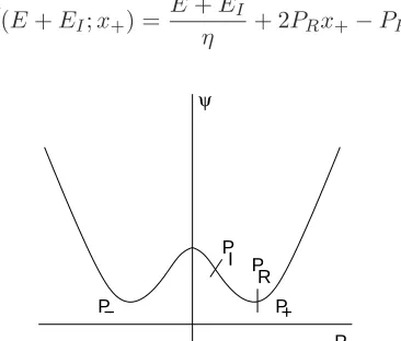
wherePI =PR−Ec/η denotes the positive inflection point at which the dipoles switch orien-tation, PR is the local remanence polarization, and η is the reciprocal slope ∂E_∂P. This energy relation is plotted in Figure 2.1.

The Gibbs free energy

G=ψ₋EP (2.6)

balances this internal Helmholtz energy with the electrostatic energy; i.e., work performed by the applied external field. As detailed in [40], where the Legendre transform properties of the Gibbs energy are discussed, G is a function of the independent variable E and the dependent variableP.

For regimes in which thermal relaxation is negligible, direct minimization of (2.6) yields the kernel

P(E+EI;x+) =

E+EI

η + 2PRx+−PR (2.7)

P ψ

+ P P−

P I

R P

(23)

where x+ = 1 for positively oriented dipoles and x+ = 0 for negatively oriented dipoles. For

algorithm development,x+ is set to 1 wheneverE+EI > Ec and to 0 whenever E+EI <−Ec. Thermal activation is manifested by dipoles having sufficient thermal energy to switch states before a minima of the Gibbs energy is eliminated. To quantify this, the Gibbs energy is balanced with the relative thermal energy through Boltmann’s relation

µ(G) =Cexp

−GV_kT

(2.8)

where V is the mesoscopic reference volume, k is Boltzmann’s constant, T is the material temperature in Kelvin, and C is a constant chosen to ensure integration to unity. It is shown in [40, 41, 46] that the resulting kernel is

P =x+hP+i+ (1−x+)hP−i (2.9)

wherex+∈[0,1] denotes the fraction of positively oriented dipoles and

hP+i= R∞

PI Pexp

−G(E+EI,P)V

kT

dP R∞

PI exp

−G(E+EI,P)V

kT

dP

, _hP−i=

R−PI

−∞ Pexp

−G(E+EI,P)V

kT

dP R−PI

−∞ exp

−G(E+EI,P)V

kT

dP

(2.10)

are the average polarizations associated with positive and negative dipole orientations. The evolution of dipole fractions is governed by the differential equation

˙

x+=−p+−x++p−+(1−x+) (2.11)

where the likelihoodsp+−andp−+of a dipole switching from positive to negative, or vice-versa,

are

p+−=

exp−G(E+EI,PI)V

kT

τ(T)R_P∞

I exp

−G(E+EI,P)V

kT

dP

p−+=

exp−G(E+EI,−PI)V

kT

τ(T)R−PI

−∞ exp

−G(E+EI,P)V

kT

dP

(2.12)

and τ quantifies the material and temperature-dependent relaxation time. It is noted in [40] that whereas these likelihood relations are commonly employed in practice, they must be treated as approximate in a statistical sense. As an alternative, the formulations

p+−=

RPI+ǫ

PI exp

₋_G₍_E₊_E

I,P)V

kT

dP

τ(T)R_P∞

I exp

₋_G₍_E₊_E

I,P)V

kT

dP

p−+=

R−PI

−PI−ǫexp

₋_G₍_E₊_E

I,P)V

kT

dP

τ(T)R−PI

−∞ exp

₋_G₍_E₊_E

I,P)V

kT

dP

(2.13)

(24)

2.2 Comparison of Response to Data

The homogenized energy model has been extensively validated against data from a wide range of actuators [5, 10, 40, 46]. Since our focus is computational rather than experimental, we briefly illustrate its performance by comparing it to steel, PLZT, and Terfenol-D actuators. Fig-ures 2.2(b) and (c) show a fit to a cylindrical steel rod for the input in Figure 2.2(a), as reported in [5]. A fit to creep data on this same rod is given in Figures 2.2(e) and (f). Representative fits for PLZT and Terfenol-D data are given in Figure 2.3.

2.3 Homogenized Energy Model Implementation

The average polarization relations (2.10) and switching likelihood relations (2.12) are compu-tationally expensive to compute, especially since they must be computed at each quadrature point and each time step. However, the choice of a piecewise quadratic Helmholtz energy, as opposed to a single fourth-order polynomial or other function, poses several advantages. One advantage is it allows these average polarizations and switching likelihoods to be expressed in a more computationally efficient form. To simplify notation, letEe=E+EI denote the effective field. Consider the integral _Z

∞

PI

exp

−G(Ee, P)V

kT

dP.

By completing the square, this is equivalent to

s πkT

2V η exp

V η

2kT

E_e2

η2 + 2PR

Ee

η

erfc

V η

2kT

PI−PR−

Ee

η

. (2.14)

The likelihood of switching from positive to negative can thus be formulated as

p+−=

√

2V η

τ(T)√πkTerfcx₂V η_kT PI−PR− E_ηe

. (2.15)

Similarly, the fundamental theorem of calculus may be applied toR_P∞

I Pexp

−GV kT

dP to obtain

hP+_i=

√

2kT

√

πV ηerfcx₂V η_kT PI−PR−E_ηe

+ Ee

η +PR. (2.16)

Similar approaches may be taken for the other average polarization and switching likelihood. Introducing the change of variables

z+=

s V

2kT η(−E−EI−Ec), z−= s

V

(25)

0 10 20 30 40 50 −60

−40 −20 0 20 40 60

time (s)

Magnetic Field (KA/m)

−15 −10 −5 0 5 10 15 −600

−400 −200 0 200 400 600

Magnetization (KA/m)

model data

(a) (b)

−0.5 0 0.5 1 1.5 2 2.5 3 3.5 −200

−100 0 100 200 300 400

model data

0 10 20 30 40 50

−60 −40 −20 0 20 40 60

time (s)

(c) (d)

0 10 20 30 40 50

−600 −400 −200 0 200 400 600

time (s)

model data

, 41.5 42 42.5 43 43.5 44 44.5 45 45.5 46 130

140 150 160 170 180 190 200 210

time (s)

model data

(e) (f)

(26)

−0.8 −0.6 −0.4 −0.2 0 0.2 0.4 0.6 0.8 −0.25 −0.2 −0.15 −0.1 −0.05 0 0.05 0.1 0.15 0.2 0.25

Electric Field (MV/m)

Polarization (C/m

2)

Model Data

−20 −10 0 10 20 −400 −300 −200 −100 0 100 200 300 400

Magnetic Field (kA/m)

Magnetization (kA/m)

Model Data

(a) (b)

Figure 2.3: Comparison of model versus data for (a) PLZT and (b) Terfenol-D. PLZT data is taken from [20] whereas Terfenol-D data is courtesy of Marcelo Dapino at The Ohio State University.

yields the relations

p+− =

1

τ(T)

r

2V η πkT

1 erfcx(z+)

, _hP+_i=

s

2kT πV η

1 erfcx(z+)

+ E+EI

η +PR,

p−+ =

1

τ(T)

r

2V η πkT

1 erfcx(z−)

, _hP_−i=₋

s

2kT πV η

1 erfcx(z−)

+E+EI

η −PR.

(2.18)

Since the scaled complementary error functions appear in both switching likelihoods and average polarizations, the values need only be computed once instead of twice. To this end, define

pos= 1

erfcx(z+)

, neg= 1

erfcx(z−)

. (2.19)

The model can then be expressed as

P(E;x+) =

E

η −PR+

Nc X i=1 NI X j=1

wc[i]wI[j] (x+(pos+neg+k1)−neg) (2.20)

where

wc[i] =p2kT /πV ηνc(Ec[i])wc[i], wI[j] =νI(EI[j])wI[j], k1=PR

p

2πV η/kT .

We note that the relations

Z ∞

−∞

Z ∞

0

νc(Ec)νI(EI)dEcdEI = 1,

Z ∞

−∞

Z ∞

0

(27)

were used to simplify the equations resulting from the physical constraints (2.3). Similarly the evolution of dipole fractions is given by

˙

x+=

1

k2

(₋x+(pos+neg) +neg) (2.21)

where

k2 =τ(T)

s πkT

2V η.

The differential equation (2.21) may be solved by any number of numerical differential equa-tions routines. For example, using the backward Euler method, x+ is computed at each time

step as

x+(t+ ∆t) =

k2

∆tx+(t) +neg k2

∆t+neg+pos

. (2.22)

A more accurate, but also slightly more computationally intensive approximation, can be solved by assumingE(t) is constant betweentandt+ ∆t; that is, approximateE(t) by a step function, as is often the case in a digital system. In this case, the differential equation is a linear constant coefficient equation, and can be solved analytically to obtain

x+(t+ ∆t) = neg

neg+pos+

x+(t)− neg

neg+pos

exp

−∆_kt

2

(neg+pos)

. (2.23)

Whereas more accurate, the difference between the solution values provided by this formulation and (2.22) is typically not significant. For example, Figure 2.4 shows the results of both methods for an example input and parameter set (in this case, taken to match the ferroelectric material PLZT). As can be seen in the magnified version, the difference between the methods is minimal. For most applications, (2.22) is considered sufficiently accurate and we employ this approach due to its greater computational simplicity.

The formulations given here can significantly improve the run-time of the algorithm as com-pared with a more direct implementation of the equations in Section 2.1. However, in many cases better performance is still required. This leaves two options: reduce the number of quadrature points or consider additional approximation strategies.

2.4 Quadrature and the Continuity of P

It is observed that the computation time of the model is directly proportional to NcNI, the number of quadrature points. One may hope to improve computational performance by reducing the number of quadrature points. However, this exaggerates actual or apparent discontinuities in the outputP.

(28)

−0.5 0 0.5 −0.25

−0.2 −0.15 −0.1 −0.05 0 0.05 0.1 0.15 0.2 0.25

Polarization (C/m

2)

Backward Euler Analytic

−0.1 −0.05 0 0.05 0.1 0.15 0.2 0.25 0.05

0.06 0.07 0.08 0.09 0.1 0.11

Polarization (C/m

2)

Backward Euler Analytic

(a) (b)

Figure 2.4: Comparison between the backward Euler approximation (2.22) and analytic ap-proximation (2.23) for an example input, with parameters taken to match PLZT. (a) Entire hysteresis curve, and (b) magnified view.

finite sums,P is smooth if and only if P is smooth for every quadrature point. Clearly for the negligible relaxation case (2.7),P is discontinuous, and its value changes by 2PRat the coercive pointE+EI =Ec. Thus,P contains NcNI finite jumps, each of size

2PRνc(Ec[i])νI(EI[j])wc[i]wI[j], i= 1. . . Nc, j = 1. . . NI.

For the relaxation case, it can be shown thatP(E;x+) is a continuous function. However, a

plot ofP(E;x+) (or ratherM(H;x+) since the parameters come from a least-squares data fit to

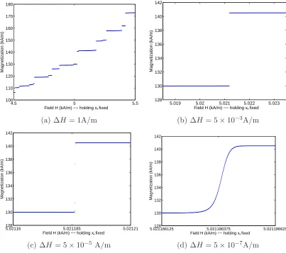
a Terfenol-D rod) shows that extremely small stepsizes may be required to resolve this continuity. Figure 2.5(a) shows a plot of M(H;x+) for various values of H where the state x+ was held

fixed; i.e., each plotted sample was obtained by inputting the given H to the model with the same value ofx+. The step between each input value of H was 1 A/m, and the function appears

to be discontinuous. However, zooming in on one of these regions shows that the function is in fact continuous (see Figures 2.5(b) – 2.5(d)). Note, however, that it takes a ∆H approximately 10 orders of magnitude belowH to resolve the function in detail. It is unrealistic to expect such steep slopes to be resolved numerically. In practice, therefore, we must allow for the relaxation model to be discontinuous as well.

Model-based control applications require a smooth model response. As detailed in [40], the relaxation model limits to the negligible relaxation model as _kTV _{→ ∞}. Since, the jump discontinuities in the negligible relaxation model are of height

2PRνc(Ec[i])νI(EI[j])wc[i]wI[j], i= 1. . . Nc, j = 1. . . NI,

(29)

approxi-4.5 5 5.5 100

110 120 130 140 150 160 170 180

Field H (kA/m) −− holding x+ fixed

5.019 5.02 5.021 5.022 5.023 128

130 132 134 136 138 140 142

(a) ∆H= 1A/m (b) ∆H= 5_×10−3A/m

5.02116 5.021185 5.02121

128 130 132 134 136 138 140 142

5.021186125128 5.021186375 5.021186625 130

132 134 136 138 140 142

(c) ∆H= 5_×10−5 _A/m _{(d) ∆}_H_{= 5}_×₁₀−7_A/m

Figure 2.5: Plot ofM(H;x+) for 6 intervals of composite 4-point Gaussian quadrature on each

density. For each value ofH,x+was held fixed; thus the plots represent a single timestep of the

model for various input levels. The parameters in these plots were taken from a least-squares fit to Terfenol-D data.

mately this height. Thus, the actual or apparent discontinuities may be minimized by minimizing

νc(Ec[i])νI(EI[j])wc[i]wI[j].

One way to increase smoothness is thus to increase the number of quadrature points. If the densities remain unchanged and the number of quadrature points is doubled, then wc[i]wI[j] is halved for all i, j. This cuts the size of the jump in half. However, computation time is proportional to the number of quadrature points, so halving the height of the jumps in this way doubles the computation time. This is clearly undesirable. A better situation can be obtained if care is taken on how the quadrature is performed.

(30)

the subintervals are taken to be equally spaced and this approach was used in the plots given previously. However, equally spaced subintervals are merely a convenience – there is no theo-retical reason why one subinterval cannot be bigger than another. In particular, if the region is partitioned such that the integral over each subinterval is equal, thenνc(Ec[i])νI(EI[j])wc[i]wI[j] will be on the same order of magnitude for all i, j. (Equality is not obtained because νc and

νI vary on the interval and because for a general quadrature formula not all the weights are equal.) This has the effect of leveling out the jumps, decreasing the big ones while the small ones increase. The result is depicted in Figure 2.6.

The required number of quadrature points is often determined by accuracy and smoothness requirements. This approach can reduce the number of quadrature points needed for a given smoothness, resulting in significant computational savings.

2.5 Approximation Methods for Improved Computational

Per-formance

Reduction of quadrature points alone is not always sufficient to achieve the desired performance of the relaxation model. Significant savings can also be obtained by introducing numerical approximations into the kernel itself. Exploration of the kernel shows that the majority of com-putation time is spent in the calculation of (2.19), and we thus focus on methods to approximate

4.5 5 5.5

100 110 120 130 140 150 160 170 180

Equally spaced intervals Unequally space intervals

Figure 2.6: Comparison ofM(H;x+) for 6 intervals of composite 4-point Gaussian quadrature

(31)

posand neg. This is equivalent to approximating

f(z) = 1

erfcx(z) (2.24)

since bothpos and neg require this function for different values of z. The rest of the model is employed in the manner detailed previously.

2.5.1 Look-up Tables

The simplest approach conceptually is to store f(z) in a table for values of interest and ap-proximate pos and neg by looking up the table value nearest z+ and z−, respectively. At the

cost of memory, this reduces the complex erfcx calculation to a simple index calculation and memory access. The indexes into the lookup table may also be calculated efficiently. Let h be the difference inz between two elements of the table, and letℓbe thez value corresponding to the first (lowest) table entry. Then define

˜

Ec[i] =

Ec[i]

h s

V

2kT η − ℓ

h, i= 1. . . Nc, E˜I[j] =

EI[j]

h s

V

2kT η, j= 1. . . NI,

˜

E = E

h V

2kT η.

Most of these calculations can be performed offline. Only ˜E needs to be computed at each time step and this may be done outside the loops over the quadrature points. Once these values are obtained, the table index is obtained by rounding

pos index=₋E˜₋E˜I[j]₋E˜c[i], neg index= ˜E+ ˜EI[j]₋E˜c[i] (2.25)

to the nearest integer. These values must be checked against the table bounds. An index less than zero signifies a zero should be given instead of a value from the table, whereas an index greater than or equal to the table size implies that the linear approximation should be used instead. Note that the linear approximation for largerz can be adjusted to take the table index (preferably without rounding) instead of thez+ or z− as input as well, allowing ˜Ec and ˜EI to replace the memory taken by the original quadrature points.

(32)

using IEEE double precision floating point numbers. Finally, table values do not need to be recalculated if material properties (i.e., temperature) change. However, there are architectures where this moderate amount of memory is unattainable, or where memory access is too slow. For these cases, we alternatively consider polynomial approximations.

2.5.2 Rational Chebyshev Approximation

If the look-up table approximation is infeasible, the functionf(z) can instead by approximated by a polynomial or a rational function

Rmk(z) = pm(z)

qk(z) (2.26)

wherep is a polynomial of degreemand qis a polynomial of degree k. HereRmk is chosen such that

maxw(z)f(z)₋Rmk(z)

(2.27)

is minimized. This is referred to as a rational Chebyshev or minimax approximation, and is the approach used to implement erfc internally as well. While it can be shown that a unique min-imix approximation exists for all mand k, computation of these approximations in numerically intensive [36]. However,f(z) does not depend on the material parameters or inputs. Thus, the minimax approximation can be calculated in advance and made available to the code for any choice of parameters. Methods to calculate these approximations using the Remez (also called Remes) algorithm are available in bothMathematicaandMaple, alleviating the user from coding minimax algorithms themself.

Like the look-up table, the minimax approximation is applied on a bounded interval. Ad-ditionally, the weight function w(z) must be specified. The obvious choices are w(z) = 1 for absolute error orw(z) = 1/f(z) for relative error. For larger z, relative error is a better met-ric for controlling error. However, for small z calculation of relative error is problematic since

f(z)_−→0. Thus, we let

w(z) = min

1, erfc(z)

exp(₋z2₎

(2.28) to use relative error for largerz and absolute error for smaller z. The transition from absolute to relative error occurs at z= 0 and w(z) is continuous.

(33)

letf(z) be approximated as

f(z)_≈

                  

0 z <₋3

Rℓ(z) =

pℓ0+pℓ1z+pℓ2z2+pℓ3z3

qℓ0+qℓ1z+qℓ2z2 −

3_≤z_{≤ −}1₂

Rh(z) = ph0+ph1z+ph2z

2₊_p

h3z3

qh0+qh1z+qh2z2 −

1

2 < z≤25

mz+b z_≥25.

(2.29)

This employs two minimax approximations with a degree 3 numerator and degree 2 denominator where the regions for each approximation were chosen so that the minimax error (2.27) is approximately the same. This holds the error (2.27) below 4_×10−4 _{for all} _{z <} _{25. Since}

this accuracy is well above the limits imposed by IEEE double precision floating point numbers, further computational savings may be realized by transformingRℓ(z) andRh(z) into continued fraction form, namely

Rℓ(z) =aℓ0const+aℓ0linz+

bℓ1

z+aℓ1+z+bℓa2ℓ2

, Rh(z) =ah0const+ah0linz+

bh1

z+ah1+z+bha2h2

.

(2.30) Note that for each of these evaluations only 1 multiply, 2 divides, and 5 additions are required. The values of the relevant coefficients are given in Table 2.1.

2.5.3 Method Comparisons

(34)

Table 2.1: Coefficients for the minimax approximation given in (2.29).

m 1.771048244745112288944163714 b 0.0705327380461303718160865974

aℓ0const 1.05305341778847673369961876455 aℓ0lin 0.141908467579507101523861449079

aℓ1 0.652521450575033268529746994429 bℓ1 2.05040334028682659509776710501 aℓ2 -0.139674180341575164555785667908 bℓ2 2.88659338549683880846513610339 ah0const 0.0568934411527620915320982226406 ah0lin 1.77070610668997459554647064088

ah1 -12.9327277303294522316468471279 bh1 0.269387658595592656676548244377 ah2 16.4152526433497348583844713265 bh2 216.983649137026313567944222991

Table 2.2: Time steps per second computed by full-precision, look-up table, and rational Chebyshev algorithms for three different computer architectures (averaged from 1 million time step). Polynomial approximation was performed using the continued fraction form (2.30) of the example polynomial given in (2.29). Look-up tables were computed for ₋6 _≤ z _≤ 25. In all cases, the model was run with 40 quadrature points for each distribution (1600 total).

Intel Xeon Intel Xeon (64 bit) Intel Pentium-M

1.7 GHz 3.8 GHz 2.16 GHz

256 KB L2 Cache 2 MB L2 Cache 2 MB L2 Cache

Negligible relaxation 10,748 62,725 31,969

algorithm

Relaxation – full numerical 429 1801 1276

precision

Relaxation – look-up table 5344 14,923 14,226

approximation

Relaxation – polynomial 4997 11,674 12,177

approximation (2.29)

Table 2.3: Approximation error for an example input using parameters obtained for PLZT. Polynomial approximation was performed using the continued fraction form (2.30) of the example polynomial given in (2.29); look-up tables were computed for ₋6_≤z_≤25, and erfcx was implemented directly as exponential and error function evaluations, with the linear approx-imation utilized for largez. Forty quadrature points were given for each distribution (1600 total)

Peak error (% ofPR) RMS error (% of PR) Look-up table (100 table elements) 0.65860% 0.25593%

(35)

2.6 Displacement Model

Whereas polarization or inductance/magnetization can sometimes be measured, it is often neces-sary to formulate the model in terms of displacement instead of polarization. Any such extension requires knowledge of the geometry of the transducer. Rods or beams can be treated with a one-dimensional transducer model, whereas more general shapes require higher-dimension models. As detailed in [40], both nanopositioning stages employed in common atomic force microscope designs and magnetic transducers employed for high speed milling utilize ferroelectric and ferro-magnetic rods that are clamped at one end and subject to damped restoring forces at the other. Hence we illustrate the model for a rod of length ℓ and cross sectional area A as depicted in Figure 2.7. The end mass mℓ with dampingcℓ and stiffness kℓ encompass adjacent transducer and plant dynamics.

It is shown in [40] that the constitutive relation for the induced stress is given by

σ=Y ε+Cε˙₋a1(P−P0)−a2(P−P0)2 (2.31)

whereY is the Young’s modulus of the transducer, C is the Kelvin-Voight damping coefficient,

P0 is the point the material is poled around,a1 and a2 are constants of proportionality relating

the induced polarization to mechanical force, andP =P(E;x+) is given in (2.4).

Due to the distributed nature of the device, partial differential equation models have been developed in [40, 43] to characterize the device dynamics. However, for a number of motivating applications, it has been shown that because forces and fields are uniform in space, strains and hence displacements are also uniform thus permitting the use of ordinary differential equation representations. In this case, the strain is given by

ε(t) = u(t)

ℓ (2.32)

whereu(t) denotes the displacement of the rod tip at timet. A force balance yields

md

2_u

dt2 +c

du

dt +ku=α1(P −P0) +α2(P−P0)

2 _(2.33)

(36)

whereρ is the density of the rod and

m=ρAℓ+mℓ, c=

CA

ℓ +cℓ, k=

Y A

ℓ +kℓ,

α1 =Aa1, α2 =Aa2.

Further details as well as models for additional geometries may be found in [40, 43].

The solution to this differential equation can be obtained with a variety of numerical methods. However, variable-step methods require that P be known at arbitrary times, which in turn requires that the homogenized energy model be solved at arbitrary times. This is typically not feasible in practice. We thus focus on fixed time-step methods. Of these, the most accurate approximation for a given stepsize may be obtained by assuming thatP is fixed between time steps so (2.33) can be solved analytically. This is an approximation, since thermal effects dictate

P will vary with time even if E is constant; however, all other fixed step methods implicitly make similar assumptions and include additional approximation error as well.

The approximation of (2.33) depends on the relation of c2

m2 to 4_mk. First, to simplify notation,

let

v= a1

m (P−P0) +

a2

m (P −P0)

2_. _(2.34)

Here v is assumed to be a constant, although the value of the constant changes at each time step. Additionally, let

˜

k= k

m, ˜c=

c

m.

If ˜c2 >4˜k then the solution is given by

u(t) =b1exp

−1 2 ˜ c+ q ˜

c2₋_4˜_k

t

+b2exp −1 2 ˜ c₋ q ˜

c2₋_4˜_k

t

. (2.35)

Again, to simplify notation letz=pc˜2₋_4˜_k_{. Letting}_u_{(0) =}_u

0 and ˙u(0) =u1 gives

b1 = 1

2

1₋c˜

z u0−

v

˜

k

−1_zu1, b2 = 1

2

1 + ˜c

z u0−

v

˜

k

+1

zu1. (2.36)

Substitution into (2.35) and collection of like terms yields

u(t) = 1

2

1₋ ˜c

z

exp

−1₂(˜c+z)t

+

1 + ˜c

z

exp

−1₂(˜c₋z)t u0− v ˜ k +1 z exp −1

2(˜c−z)t

−exp

−1

2(˜c+z)t

u1+

v

˜

k.

(37)

If we assume the step ∆tis fixed, then we can define the six constants

d1 =

1 2

1₋c˜

z

exp

−1₂(˜c+z) ∆t

+

1 + ˜c

z

exp

−1₂(˜c₋z) ∆t

,

d2 =

1 z exp −1

2(˜c−z) ∆t

−exp

−1

2(˜c+z) ∆t

,

d3 =

1

k(1−d1),

d4 =

1 4

˜

c2

z −z exp

−1

2(˜c+z) ∆t

−exp

−1

2(˜c−z) ∆t

,

d5 = 1

2

1 +c˜

z

exp

−1₂(˜c+z) ∆t

+

1₋ ˜c

z

exp

−1₂(˜c₋z) ∆t

,

d6 =−d_˜4

k.

(2.38)

In terms of these constants, the solution of the rod model for ˜c2 >4˜k is approximated by

u(t+ ∆t) =d1u(t) +d2u˙(t) +d3v(t+ ∆t),

˙

u(t+ ∆t) =d4u(t) +d5u˙(t) +d6v(t+ ∆t).

(2.39)

A similar approach can be taken for the other two cases. If ˜c2 _{= 4˜}_k_{, we again obtain (2.39)}

except with the constants given by

d1 =

1 + ˜c 2∆t

exp

−˜c

2∆t

, d4 =−k∆texp

−˜c

2∆t

,

d2 = ∆texp

−˜c

2∆t

, d5 =

1₋c˜ 2∆t

exp

−˜c

2∆t

,

d3 =

1

k(1−d1), d6 =−

d4

˜

k .

(2.40)

Finally, if ˜c2 <4˜k, the values for the constants are

d1 = exp

−₂˜ct cosz 2∆t

+ ˜c

zsin

_z

2∆t

, d2 =

2

zexp

−c₂˜t

sinz 2∆t

,

d3 =

1

k(1−d1), d4 =−

1 2

z+c˜

2

z

exp

−₂˜ct

sinz 2∆t

,

d5 = exp

−˜c

2t cos

_z

2∆t

− ˜c

zsin

_z

2∆t

, d6 =−

d4

˜

k.

(38)

Chapter 3

Inverse Model

As discussed in Chapter 1, one method to accurately control a smart material actuator involves the use of an inverse model or compensator in the manner depicted in Figure 3.1. Linearization in this manner allows simple control techniques including PI/PID and LQR designs to be utilized over the entire range of the actuator. Given a specified displacement, we wish to determine the field necessary to bring the actuator to that value. Such inverse compensators have previously been explored for the negligible relaxation model in [16, 40]. Here we consider a method that works for both the relaxation and negligible relaxation models.

The rod model can be inverted analytically. Solving (2.39) for v yields

v(t) = 1

d3

u(t)₋d1

d3

u(t₋∆t)₋d2

d3

˙

u(t₋∆t). (3.1) Once v has been determined, the required polarization can be determined from the quadratic formula; namely

b

P(t) =P0−

α1

2α2 ± s

α1

2α2 2

+ mv(t)

a2

(3.2)

+ +

Controller field or voltage

Inverse compensator Actuator Noise

Magnetization or displacement Reference

input

(39)

as long asα26= 0. If α2 is 0, the equation is linear and the solution is b

P(t) =P0+

m

α1

v(t). (3.3)

Note that forα2 6= 0, either polarization value is acceptable, as both give equivalent

displace-ments. However, to minimize the effects of modeling error, a single branch should always be utilized.

A definition of the inverse homogenized energy model is the following: given any valid state

x+ and any specified Pb within the operating range of the material, determine E such that P =Pb. Unlike the rod model, however, it is not feasible to invert (2.4) analytically. Thus, we reformulate the problem as numerical root finding, namely determining the valueE such that for a givenx+ andPb,

P(E;x+)−Pb= 0. (3.4)

We note that this function is monotone in E (holding x+ fixed). However, as discussed in

Section 2.4, the function may contain a finite number of simple jumps.

3.1 Discontinuous Root Finding

If (3.4) was continuously differentiable, the secant method would provide nearly optimal conver-gence to the solution in terms of function evaluations [19]. However, for a discontinuous function it may not converge. The bisection method will converge, but often this convergence is slow. Methods exist that combine bisection with interpolation to attempt to improve this rate; see [6] for example. However, we observe better performance by exploiting the monotone nature of the function to directly improve the convergence of the bisection method.

The bisection method, or any other method which utilizes it, requires both that the root be bounded and that the function change signs within the bounds. For a monotone function, these requirements are the same. Theoretical bounds onE may be computed by considering the case when all dipoles have switched. In these cases (all dipoles positive or all negative), E can be determined analytically. The required value of E is by necessity between these extreme cases, namely

η(Pb₋PR)_≤E _≤η(Pb+PR). (3.5) However, direct application of the bisection method with these bounds yields slow convergence because the bounds are large.

(40)

approximation to E is obtained, or it steps too far. In this latter case, the iterations have crossed over the root value and provide a bound on the root. We therefore apply the secant method to (3.4) first. If there is sufficient relaxation or the value Pb does not lie near any discontinuities, we obtain rapid convergence. If the secant method fails to converge, the secant iterations themselves are utilized to determine the bound on the root which can then be given to bisection to find the actual root. These bounds are typically much tighter than (3.5), which improves the convergence of the bisection method. For the purposes of our algorithm, failure to converge in the secant method is defined as

|P(Ei;x+)−Pb| ≥ |P(Ei−2;x+)−Pb|, for alli≥3 (3.6)

whereEiis the value ofE determined by the ith iteration of the secant method. Such a definition is a heuristic to detect failure quickly without penalizing a single poor step.

The secant method requires an initial approximation to the derivative to compute its first iteration. One such approximation is 1/η which is the derivative if no dipoles are switching. The actual derivative may be much larger than this, but will never be smaller. Another approximation involves using the previous two time steps of the model in a manner analogous to how the secant method itself approximates derivatives. This approximation is simply ∆P/∆E, where ∆P is the difference inP(E;x+) for the previous two time steps and ∆E is the corresponding differences

inE. The latter approximation is deemed more accurate and is utilized when the previous two time steps are known. When this is not the case, 1/η is utilized as the initial derivative. The computed derivative value should also be checked against this lower limit on each iteration of the secant method, to trap some errors that may arise with the subtraction of nearly equal numbers.

3.2 Validation and Performance

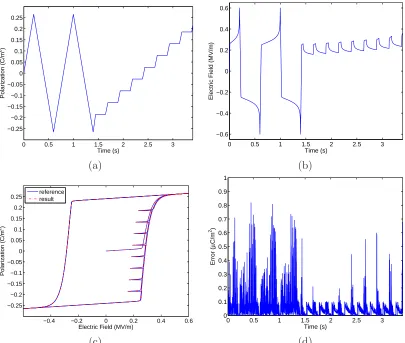
The performance of the inverse model is largely dependent on the material parameters being utilized. More relaxation, smaller variances inνc and νI, and slowly changing reference inputs generally yield better performance than small relaxation, highly variable distributions, or rapidly varying inputs. As an example, consider the inverse model results in Figure 3.2 for the stepped polarization shown in Figure 3.2(a). The parameters are specified as those estimated for PLZT to obtain the model fit in Figure 2.3(a). Ten intervals with 4-point Gaussian quadrature are utilized for each distribution and the time step is ∆t= 0.001. As can be seen, the inverse model accounts for the relaxation in the device, decreasing the electric field as appropriate to hold the polarization constant. The error between the specified and actual values is small – five orders of magnitude below the remanence polarization.

(41)

0 0.5 1 1.5 2 2.5 3 −0.25

−0.2 −0.15 −0.1 −0.05 0 0.05 0.1 0.15 0.2 0.25

Time (s)

Polarization (C/m

2)

0 0.5 1 1.5 2 2.5 3 −0.6

−0.4 −0.2 0 0.2 0.4 0.6

Time (s)

(a) (b)

−0.4 −0.2 0 0.2 0.4 0.6 −0.25

−0.2 −0.15 −0.1 −0.05 0 0.05 0.1 0.15 0.2 0.25

Polarization (C/m

2)

reference result

0 0.5 1 1.5 2 2.5 3 0

0.1 0.2 0.3 0.4 0.5 0.6 0.7 0.8 0.9 1

Time (s)

Error (

µ

C/m

2)

(c) (d)

Figure 3.2: (a) Reference polarization and (b) electric field E given by the inverse model with parameters estimated for PLZT. (c) Comparison of the resulting polarizationP and the reference polarizationPb. (d) Absolute error_|Pb₋P_|.

Table 3.1: Effort to compute the inverse model in terms of average and maximum number of function evaluations for various error tolerances, using parameters for PLZT and the input given in Figure 3.2(a). _† denotes that due to discontinuities, some time steps did not converge within the specified tolerance, and only those that did are averaged. In these cases, the maximum number of function evaluations was the user-specified maximum.

Average Maximum

Tolerance Function Evaluations Function Evaluations

PR×10−2 = 0.0024 1.0855 3

PR×10−3 = 0.00024 1.2667 4

PR×10−4 = 2.4×10−5 2.0157 5

PR×10−5 = 2.4×10−6 3.5423 9

(42)

with only 2 function evaluations (evaluations of the forward homogenized energy model) per iteration on average, or 5 in the worst case. However, this efficiency is dependent on the input. Figure 3.3(a) shows an input polarization which changes at roughly an order of magnitude higher rate. Using the same material parameters and time step on this input yields the results in Figure 3.3(b) and Table 3.2. The same accuracy level as before requires almost 5 function evaluations on average and 16 in the worst case. While increased, this is still easily attainable. The level of effort also depends on the material being modeled. Scaling Figure 3.3(a) to an appropriate level and applying parameters for a Terfenol-D rod yields the results in Figure 3.4 and Table 3.3. The Terfenol-D parameters require greater work for the same level of accuracy, but relatively speaking they are able to achieve a greater accuracy than that achieved in the PLZT case.

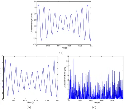
Finally, we note that these observations apply directly to the case when displacement is uti-lized as input. Figure 3.5 and Table 3.4 show the accuracy and level of effort for the Terfenol-D parameters with strain (displacement) as an input. The tolerance for the root finding algorithm was also specified in terms of displacement in this case, withP(E;x+) input to the rod model

on each iteration of secant or bisection to determine the error. We note that the inverse com-pensator provides an accurate way to control the device while maintaining a reasonable number of computations.

0 0.05 0.1 0.15 0.2 −0.25

−0.2 −0.15 −0.1 −0.05 0 0.05 0.1 0.15 0.2 0.25

Time (s)

Polarization (C/m

2)

0 0.05 0.1 0.15 0.2 −0.5

−0.4 −0.3 −0.2 −0.1 0 0.1 0.2 0.3 0.4 0.5

Time (s)

(a) (b)

(43)

0 0.05 0.1 0.15 0.2 −300

−200 −100 0 100 200 300

Time (s)

0 0.05 0.1 0.15 0.2 −20

−15 −10 −5 0 5 10 15 20

Time (s)

(a) (b)

Figure 3.4: (a) Reference magnetization and (b) magnetic field H given by the inverse model with parameters estimated for Terfenol-D.

Table 3.2: Effort to compute the inverse model in terms of average and maximum number of function evaluations for various error tolerances, using parameters for PLZT and the input given in Figure 3.3(a). _† denotes that due to discontinuities, some time steps did not converge within the specified tolerance, and only those that did are averaged. In these cases, the maximum number of function evaluations was the user-specified maximum.

Average Maximum

PR×10−2 = 0.0024 2.8776 10

PR×10−3 = 0.00024 3.9286 13

PR×10−4 = 2.4×10−5 4.8027 16

PR×10−5 = 2.4×10−6 7.9252† user-defined

PR×10−6 = 2.4×10−7 9.3187† user-defined

Table 3.3: Effort to compute the inverse model in terms of average and maximum number of function evaluations for various error tolerances, using parameters for Terfenol-D and the input given in Figure 3.4(a).

Average Maximum

MR×10−2 = 3400 2.8673 9

MR×10−3 = 340 5.4354 16

MR×10−4 = 34.0 10.7143 22

MR×10−5 = 3.40 14.2993 25

(44)

0 0.02 0.04 0.06 0.08 0.1 −20

−10 0 10 20 30 40 50

Time (s)

Displacement (microns)

(a)

0 0.02 0.04 0.06 0.08 0.1 −2

−1 0 1 2 3 4 5

Time (s)

0 0.02 0.04 0.06 0.08 0.1 0

2 4 6 8 10 12 14 16 18

Time (s)

Displacement Error (pm)

(b) (c)

Figure 3.5: Results for the combined inverse model with parameters estimated for a Terfenol-D rod. (a) Specified displacementuband (b) magnetic fieldH provided by the inverse algorithms. (c) Absolute error_|u_b₋u_|for displacement u given by the rod model.

Table 3.4: Effort to compute the inverse model in terms of average and maximum number of function evaluations utilizing parameters estimated for a Terfenol-D rod and the reference displacement given in Figure 3.5(a).

Error Average Maximum

tolerance model evaluations model evaluations

1 micron 2.1240 8

100 nm 2.2880 9

10 nm 6.5170 19

1 nm 11.6500 22

100 pm 14.7040 25