Generalized Conditionally Autoregressive Models

(1)

ABSTRACT

KYUNG, MINJUNG. Generalized Conditionally Autoregressive Models. (Under the direction of Sujit K. Ghosh.)

In many studies, lattice or area data are observed and spatial analysis is performed. A

spatial process observed over a lattice or a set of irregular regions is usually modeled

using a conditionally autoregressive (CAR) model. The neighborhoods within a CAR

model are generally formed using only the inter-distances or boundaries between the

regions. To accommodate the effect of directions, a new class of spatial models is

developed using different weights given to neighbors in different directions. The

pro-posed model generalizes the usual CAR model by accounting for spatial anisotropy.

Maximum likelihood (ML) estimators are derived and shown to be consistent and

asymptotically normal under some regularity conditions. Also, the posterior

distri-bution of the parameters are derived using conjugate and non-informative priors.

Effi-cient MCMC sampling algorithms are provided to generate samples from the marginal

posterior distribution. Simulation studies are presented to illustrate the finite sample

performance of the new model as compared to CAR model. The method is

demon-strated using a data set on the crime rates in Columbus, OH. Further generalization

of the directional CAR model is proposed that adaptively chosen the neighborhoods

based on a smooth function of the inter-distances and inter-angles between the

re-gions. The parameters of this generalized CAR are estimated using ML and Bayes

estimators. A data set on the prevalence of elevated blood lead levels of children

under the age of six years observed in the state of Virginia is used to illustrate the

(2)

Generalized Conditionally Autoregressive Models

by

Minjung Kyung

A dissertation submitted to the Graduate Faculty of North Carolina State University

in partial fulfillment of the requirements for the Degree of

Doctor of Philosophy

STATISTICS

Raleigh, North Carolina

2006

APPROVED BY:

Dr. Sujit K. Ghosh Dr. Marcia Gumpertz

Chair of Advisory Comittee

(3)

(4)

Biography

Minjung Kyung was born in Seoul, South Korea in 1976. Minjung earned her B.S. of

Statistics in 2000 from Duksung Women’s University in Seoul. She joined Department

of Statistics, Rutgers, the State University of NJ in 2000 and took her M.S. in 2003.

In 2003, she entered graduate school at North Carolina State University in Raleigh.

(5)

Acknowledgements

First of all, I would like to thank my family and friends for their love and support.

I am very fortunate to have such wonderful people in my life. They have always

encouraged me to achieve my goals and helped me to get through tough times. I

would have not finished my study at NC State without them.

I also would like to express my deepest gratitude and biggest appreciation to my

advisor Dr. Sujit K. Ghosh. He has been of great help for me to write this thesis. I

have learned so much from him.

My committee members, Dr. Gumpertz, Dr. Fuentes and Dr. Zhang, have been

very helpful. I would especially like to thank them for their comments on this thesis.

(6)

List of Tables

1.1 Performance of MLE’s of ρ’s and σ2_{’s . . . .} ₂₂

1.2 Performance of Bayesian estimates ofρ’s and σ2_{’s . . . .} ₂₄

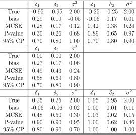
2.1 Performance of MLE’s of δ1’s,δ2’s and σ2’s . . . 45

2.2 Performance of Bayesian estimates ofδ1’s, δ2’s and σ2_{’s . . . .} ₄₇

2.3 Performances of MLE of DCAR model withN = 500 data sets gener-ated from CAR process . . . 50

2.4 Performance of Bayesian estimates of the DCAR model with 10 data sets generated from CAR process . . . 52

2.5 Compariosn of AIC, BIC and DIC between CAR and DCAR models with data sets from CAR process (PCD = Percentage of Correct Decision) 53 2.6 Performances of MLE of CAR model withN = 500 data sets generated from DCAR process . . . 55

2.7 Performance of Bayesian estimates of the DCAR model with 10 data sets generated from CAR process . . . 56

2.8 Compariosn of AIC, BIC and DIC between CAR and DCAR mod-els with data sets from DCAR process (PCD = percentage of correct decisions) . . . 58

2.9 Linear model of house value and income on log transformed crime rate of Columbus OH without outliers (Model 1) . . . 62

2.10 Estimated crime rate of Columbus OH with CAR and DCAR model for the latent spatial process without outliers (Model 2-3) . . . 62

2.11 Mean Squared Predicted Error of Leave-one-out method (MSPE) . . 64

3.1 ML estimates of β and σ2_{’s and ESE’s . . . .} ₇₉

3.2 Performance of MLE’s of GCAR model . . . 81

3.3 Performance of Bayesian estimates of GCAR model . . . 83 3.4 Comparison of ML estimated variance-covariance matrices of CAR and

DCAR process to known variance-covariance matrix of GCAR process 84 3.5 Comparison of ML estimated variance-covariance matrices of GCAR

(9)

3.6 Estimated elevated blood lead rates in children under 6 years of age in Virginia, 2000 . . . 90

A.1 Performances of MLE of CAR model based on data sets generated from CAR process with ρ=−0.95 . . . 107 A.2 Performances of MLE of CAR model based on data sets generated from

CAR process with ρ=−0.25 . . . 108 A.3 Performances of MLE of CAR model based on data sets generated from

CAR process with ρ= 0.00 . . . 108 A.4 Performances of MLE of CAR model based on data sets generated from

CAR process with ρ= 0.25 . . . 109 A.5 Performances of MLE of CAR model based on data sets generated from

CAR process with ρ= 0.95 . . . 109 A.6 Performances of Bayes estimates of CAR model based on data sets

generated from CAR process with ρ=−0.95 . . . 115 A.7 Performances of Bayes estimates of CAR model based on data sets

generated from CAR process with ρ=−0.25 . . . 115 A.8 Performances of Bayes estimates of CAR model based on data sets

generated from CAR process with ρ= 0.00 . . . 115 A.9 Performances of Bayes estimates of CAR model based on data sets

generated from CAR process with ρ= 0.25 . . . 116 A.10 Performances of Bayes estimates of CAR model based on data sets

generated from CAR process with ρ= 0.95 . . . 116 A.11 Performances of ML estimates of DCAR model based on data sets

generated from DCAR process withδ1 =−0.95 and δ2 =−0.97 . . . 122 A.12 Performances of ML estimates of DCAR model based on data sets

generated from DCAR process withδ1 =−0.3 and δ2 = 0.95 . . . 122

A.13 Performances of ML estimates of DCAR model based on data sets generated from DCAR process withδ1 =−0.95 and δ2 = 0.97 . . . . 123 A.14 Performances of ML estimates of DCAR model based on data sets

generated from DCAR process withδ1 = 0.95 andδ2 = 0.93 . . . 123 A.15 Performances of Bayes estimates of DCAR model based on data sets

generated from DCAR process withδ1 =−0.95 and δ2 =−0.97 . . . 128

A.16 Performances of Bayes estimates of DCAR model based on data sets generated from DCAR process withδ1 =−0.30 and δ2 = 0.95 . . . . 128 A.17 Performances of Bayes estimates of DCAR model based on data sets

generated from DCAR process withδ1 =−0.95 and δ2 = 0.97 . . . . 129 A.18 Performances of Bayes estimates of DCAR model based on data sets

generated from DCAR process withδ1 = 0.95 andδ2 = 0.93 . . . 129

(10)

A.20 Performances of ML estimates of DCAR model based on data sets generated from CAR process with ρ=−0.25 (δ1 =δ2 =ρ) . . . 134

A.21 Performances of ML estimates of DCAR model based on data sets generated from CAR process with ρ= 0.00 (δ1 =δ2 =ρ) . . . 135 A.22 Performances of ML estimates of DCAR model based on data sets

generated from CAR process with ρ= 0.25 (δ1 =δ2 =ρ) . . . 135 A.23 Performances of ML estimates of DCAR model based on data sets

generated from CAR process with ρ= 0.95 (δ1 =δ2 =ρ) . . . 135

A.24 Performances of Bayes estimates of DCAR model based on data sets generated from CAR process with ρ= 0.95 (δ1 =δ2 =ρ) . . . 141 A.25 Performances of Bayes estimates of DCAR model based on data sets

generated from CAR process with ρ=−0.25 (δ1 =δ2 =ρ) . . . 141 A.26 Performances of Bayes estimates of DCAR model based on data sets

generated from CAR process with ρ= 0.00 (δ1 =δ2 =ρ) . . . 141

A.27 Performances of Bayes estimates of DCAR model based on data sets generated from CAR process with ρ= 0.25 (δ1 =δ2 =ρ) . . . 142 A.28 Performances of Bayes estimates of DCAR model based on data sets

generated from CAR process with ρ= 0.95 (δ1 =δ2 =ρ) . . . 142 A.29 Performances of ML estimates of CAR model based on data sets

gen-erated from DCAR process with δ1 = −0.95 and δ2 = −0.97 (True ρ

is mean of trueδ1 and δ2) . . . 148 A.30 Performances of ML estimates of CAR model based on data sets

gen-erated from DCAR process with δ1 = −0.30 and δ2 = 0.95 (True ρ is

mean of true δ1 and δ2) . . . 148 A.31 Performances of ML estimates of CAR model based on data sets

gen-erated from DCAR process with δ1 = −0.95 and δ2 = 0.97 (True ρ is

mean of true δ1 and δ2) . . . 149 A.32 Performances of ML estimates of CAR model based on data sets

gen-erated from DCAR process with δ1 = 0.95 and δ2 = 0.93 (True ρ is mean of true δ1 and δ2) . . . 149 A.33 Performances of Bayes estimates of CAR model based on data sets

generated from DCAR process withδ1 =−0.95 and δ2 =−0.97 . . . 154 A.34 Performances of Bayes estimates of CAR model based on data sets

generated from DCAR process withδ1 =−0.30 and δ2 = 0.95 . . . . 154 A.35 Performances of Bayes estimates of CAR model based on data sets

generated from DCAR process withδ1 =−0.95 and δ2 = 0.97 . . . . 155 A.36 Performances of Bayes estimates of CAR model based on data sets

generated from DCAR process withδ1 = 0.95 andδ2 = 0.93 . . . 155 A.37 Linear model of house value and income on log transformed crime rate

(11)

A.38 Linear model of median housing value and poverty on the Freeman-Tukey transformed elevated blood lead levels of children under 6 in Virginia, 2000 . . . 165 A.39 Linear model of median housing value and poverty on the

(12)

List of Figures

1.1 The log-transformed crime rate of 49 neighborhoods in Columbus, OH, 1980 that are divided into 5 intervals of each 20% quantiles. . . 5

2.1 The angle (in radian)αij . . . 28

2.2 Correlogram of log transformed crime rate of Columbus OH without outliers . . . 60 2.3 Predicted Log transformed crime rate of Columbus OH (Model 2 and

Model 3: ML method) . . . 64 2.4 Residual plots of log transformed crime rate of Columbus OH (Model

2 and Model 3: ML method) . . . 65

3.1 The Freeman-Tukey transformed rate of children under 6 years of age with elevated blood lead levels into 5 intervals of each 20% quantiles. 87 3.2 Predicted Freeman-Tukey transformed blood lead level of children

un-der 6 in Virginia with GCAR model(Bayes: Model 3.2) . . . 91 3.3 Residual plots of Freeman-Tukey transformed blood lead level of

chil-dren under 6 in Virginia with GCAR model(Bayes: Model 3.2) . . . . 91

A.1 Bivariate Epanechnikov densities with negative directional correlation

α’s. . . 106 A.2 Histograms of estimated parameters of CAR models with Trueρ=−0.95.110 A.3 Histograms of estimated parameters of CAR models with Trueρ=−0.25.111 A.4 Histograms of estimated parameters of CAR models with True ρ= 0. 112 A.5 Histograms of estimated parameters of CAR models with True ρ= 0.25.113 A.6 Histograms of estimated parameters of CAR models with True ρ= 0.95.114 A.7 Posterior density of estimated parameters of CAR models using Bayesian

method with Trueρ=−0.95 . . . 117 A.8 Posterior density of estimated parameters of CAR models using Bayesian

method with Trueρ=−0.25 . . . 118 A.9 Posterior density of estimated parameters of CAR models using Bayesian

(13)

A.10 Posterior density of estimated parameters of CAR models using Bayesian method with Trueρ= 0.25 . . . 120 A.11 Posterior density of estimated parameters of CAR models using Bayesian

method with Trueρ= 0.95 . . . 121 A.12 Histograms of estimated parameters of DCAR models with δ1 =−0.95

and δ2 =−0.97. . . 124 A.13 Histograms of estimated parameters of DCAR models with δ1 =−0.30

and δ2 = 0.95. . . 125

A.14 Histograms of estimated parameters of DCAR models with δ1 =−0.95 and δ2 = 0.97. . . 126 A.15 Histograms of estimated parameters of DCAR models with δ1 = 0.95

and δ2 = 0.93. . . 127 A.16 Posterior density of estimated parameters of DCAR models using Bayesian

method with Trueδ1 =−0.95 and δ2 =−0.97 . . . 130

A.17 Posterior density of estimated parameters of DCAR models using Bayesian method with Trueδ1 =−0.30 and δ2 = 0.95 . . . 131 A.18 Posterior density of estimated parameters of CAR models using Bayesian

method with Trueδ1 =−0.95 and δ2 = 0.97 . . . 132 A.19 Posterior density of estimated parameters of CAR models using Bayesian

method with Trueδ1 = 0.95 and δ2 = 0.93 . . . 133

A.20 Histograms of ML estimates of DCAR model based on CAR process samples withρ=−0.95 . . . 136 A.21 Histograms of ML estimates of DCAR model based on CAR process

samples withρ=−0.25 . . . 137 A.22 Histograms of ML estimates of DCAR model based on CAR process

samples withρ= 0.00 . . . 138 A.23 Histograms of ML estimates of DCAR model based on CAR process

samples withρ= 0.25 . . . 139 A.24 Histograms of ML estimates of DCAR model based on CAR process

samples withρ= 0.95 . . . 140 A.25 Posterior density of Bayes estimates of DCAR models using Bayesian

method based on CAR process samples with trueρ=−0.95 . . . 143 A.26 Posterior density of Bayes estimates of DCAR models using Bayesian

method based on CAR process samples with trueρ=−0.25 . . . 144 A.27 Posterior density of Bayes estimates of DCAR models using Bayesian

method based on CAR process samples with trueρ= 0.00 . . . 145 A.28 Posterior density of Bayes estimates of DCAR models using Bayesian

method based on CAR process samples with trueρ= 0.25 . . . 146 A.29 Posterior density of Bayes estimates of DCAR models using Bayesian

method based on CAR process samples with trueρ= 0.95 . . . 147 A.30 Histograms of ML estimates of CAR model based on samples from

(14)

A.31 Histograms of ML estimates of CAR model based on samples from DCAR process with δ1 =−0.30 and δ2 = 0.95 . . . 151

A.32 Histograms of estimated parameters of DCAR samples withδ1 =−0.95 and δ2 = 0.97 by fitting CAR model. . . 152 A.33 Histograms of ML estimates of CAR model based on samples from

DCAR process with δ1 = 0.95 and δ2 = 0.93 . . . 153 A.34 Posterior density of Bayes estimates of CAR model based on samples

from DCAR process withδ1 =−0.95 and δ2 =−0.97 . . . 156

A.35 Posterior density of Bayes estimates of CAR model based on samples from DCAR process withδ1 =−0.30 and δ2 = 0.95 . . . 157 A.36 Posterior density of Bayes estimates of CAR model based on samples

from DCAR process withδ1 =−0.95 and δ2 = 0.97 . . . 158 A.37 Posterior density of Bayes estimates of CAR model based on samples

from DCAR process withδ1 = 0.95 andδ2 = 0.93 . . . 159

A.38 Log transformed crime rate of Columbus OH . . . 160 A.39 Log transformed crime rate of Columbus OH without outliers . . . . 161 A.40 Predicted Log transformed crime rate of Columbus OH (Model 1) . . 162 A.41 Residual plots of log transformed crime rate of Columbus OH(Model 1) 162 A.42 Predicted Log transformed crime rate of Columbus OH (Model 2:

Bayesian method) . . . 163 A.43 Residual plots of log transformed crime rate of Columbus OH(Model

2: Bayesian method) . . . 163 A.44 Predicted Log transformed crime rate of Columbus OH (Model 3:

Bayesian method) . . . 164 A.45 Residual plots of log transformed crime rate of Columbus OH(Model

3: Bayesian method) . . . 164 A.46 The Freeman-Tukey transformed blood lead level in Virginia . . . 166 A.47 The Freeman-Tukey transformed blood lead level in Virginia without

outliers . . . 167 A.48 Predicted Freeman-Tukey transformed blood lead level of children

un-der 6 in Virginia with linear model . . . 168 A.49 Residual plots of Freeman-Tukey transformed blood lead level of

chil-dren under 6 in Virginia with linear model . . . 168 A.50 Predicted Freeman-Tukey transformed blood lead level of children

un-der 6 in Virginia with CAR model (MLE: Model 1.1) . . . 169 A.51 Residual plots of Freeman-Tukey transformed blood lead level of

chil-dren under 6 in Virginia with CAR model (MLE: Model 1.1) . . . 169 A.52 Predicted Freeman-Tukey transformed blood lead level of children

un-der 6 in Virginia with CAR model(Bayes: Model 1.2) . . . 170 A.53 Residual plots of Freeman-Tukey transformed blood lead level of

(15)

A.54 Predicted Freeman-Tukey transformed blood lead level of children un-der 6 in Virginia with DCAR model (MLE: Model 2.1) . . . 171 A.55 Residual plots of Freeman-Tukey transformed blood lead level of

chil-dren under 6 in Virginia with DCAR model (MLE: Model 2.1) . . . . 171 A.56 Predicted Freeman-Tukey transformed blood lead level of children

un-der 6 in Virginia with DCAR model(Bayes: Model 2.2) . . . 172 A.57 Residual plots of Freeman-Tukey transformed blood lead level of

chil-dren under 6 in Virginia with DCAR model(Bayes: Model 2.2) . . . . 172 A.58 Predicted Freeman-Tukey transformed blood lead level of children

un-der 6 in Virginia with GCAR model (MLE: Model 3.1) . . . 173 A.59 Residual Freeman-Tukey transformed plots of blood lead level of

(16)

Chapter 1 Introduction to Conditionally

Autoregressive Models

In many studies, counts or averages over arbitrary regions are observed and spatial

analysis is performed. Counts or averages over arbitrary regions, i.e. regional

sum-mary data, is commonly known as lattice or area data (Cressie, 1993). Given a set of

geographical regions, observations collected over regions near to each other tend to

have similar characteristics as compared to distant regions. In geoscience, this feature

is known as the Tobler’s first law (Miller, 2004). From a statistical perspective, this

feature is attributed to the fact that the autocorrelation between the observations

collected from nearer regions tends to be higher than those that are distant. One of

the main goals of this thesis is to explore such hidden spatial autocorrelation of the

data generating process.

In this thesis, we explore several modeling strategies for lattice data. First,

(17)

ex-haustive sub-areas S1, . . . , Sn such that S = ∪n

i=1Si and Si ∩ Sj = ∅. Suppose Yi = Y(Si) denotes some form of aggregate response collected from the area Si.

Letdij =d(Si, Sj) whered(·,·) denotes a “distance” between the centroids of areasSi

and Sj, respectively. To avoid ambiguity, we will assume dii= 0 for i= 1, . . . , n. Let

ρij = Corr(Yi, Yj) denote the autocorrelation between Yi and Yj. Tobler’s first law

asserts us that ρij decrease, as dij increases. In order to model the Yi’s, we usually

consider the model

Yi =µi+ηi+ǫi, (1.1)

whereµi’s denote large-scale variations and are modeled using parametric or

nonpara-metric regression methods,µi =µ(Si,Xi) where Xi’s denote a vector of explanatory

variables specific to area Si. The ηi represents small-scale variations which are

com-monly known as spatial random effects andǫi represents conditionally independently

and identically distributed (iid) measurement errors with mean E[ǫi|X] = 0 and Var[ǫi|X] =σ2

ǫ.

In general, the problem of characterizing the spatial autocorrelation can be split

into two components, the large-scale variation µi and small-scale variation ηi. One

of the goals of this thesis is to develop flexible models for the ηi’s. To begin with,

we assume that ηi’s are conditionally independent of the Xi’s. In other words, the

distribution ofηi’s does not depend on the explanatory variableXi’s. This is certainly

a simplifying assumption which may or may not be appropriate for a given data set.

However, in this thesis we assume that the distribution ofηi’s is independent onXi’s.

In addition, we also assume that given the Xi’s, ηi’s are independent ofǫi’s.

(18)

mean and variance. Without much loss of generality, we assume a linear model of

the large-scale variation with parameter βi’s i = 1, . . . , q, i.e. µi = XT

i β, where

β= (β1, . . . , βq)T. Notice that nonlinear functions can be approximated using splines

and polynomials which can be re-written in the form of XT

i β (Wahba, 1977). From

model (1.1) it follows that

E[Y] = Xβ and

Var[Y] = σ_ǫ2I+Σ(ω), (1.2)

where Y = (Y1, . . . , Yn)T _{is the random vector of responses in a study area} _S_, _σ2 ǫ

represents the measurement error variance and ω includes spatial autocorrelation

parameters and other variance components. However, when Yi’s are discrete valued

it can be difficult to use model (1.1), but we can generalize (1.2) using link functions.

Thus, it is often easier to assume a spatial latent process, Z = (Z1, . . . , Zn)T, where

Zi =Z(Si), and to construct models around the moments of Y (Schabenberger and

Gotway, 2005). We assume that, given the latent spatial process Z,

g(E[Y|η]) = Z =Xβ+η

Var[Y|η] = σ_ǫ2I

Cov[Yi, Yj|η] = 0 for Si 6=Sj,

where η = (η1, . . . , ηn)T _{is as defined in (1.1) and} _g _{is a known strictly increasing}

link function such thatg(±∞) =±∞. Hence, the marginal moments of Y are easily obtained by using conditional mean and variance as

E[Y|X] = E[g−1(Xβ+η)|X] and

(19)

where g−1(Z) = g−1(Z1), . . . , g−1(Zn)T. Notice that when g(x) = x, (1.3) reduces to (1.2).

The latent spatial process Zi’s are usually modeled using a conditionally

autore-gressive (CAR) model (Besag, 1974 and 1975, Cressie and Chan, 1989) and a

simul-taneously autoregressive (SAR) model (Ord, 1975). These models have been widely

used in spatial statistics (Cliff and Ord, 1981, Besag and Kooperberg, 1995 and Wall,

2004). The CAR and SAR models are used to study how a particular region is

in-fluenced by its “neighboring regions”. In practical situations, it is more reasonable

to consider covariates with CAR models to account for variations due to

explana-tory variables. Thus, Zi can be written in the form of mixed model with a fixed

effect linear regression (the large-scale variation) and random effect spatial model

(the small-scale variation). Hence, the models are usually referred to as the mixed

regressive-autoregressive model. To illustrate this, we consider an example of the

crime rates, residential burglaries and vehicle thefts per thousand households in the

neighborhood of 49 neighborhoods in Columbus, OH, in the year of 1980. In this

data, Si’s are the 49 neighborhoods and S is Columbus, OH. Neighborhoods of each Si’s areSj’s that shares common borders. The crime rates,Yi’s are discreted valued,

thus logarithm can be used for a link function ofYi’s. In Figure 1.1, we plot the

log-transformed crime rates that are divided into 5 intervals of each 20% quantiles. In

this figure, darker regions represent higher crime rates. We see that there are higher

crime rates in middle areas of Columbus, OH, and lower crime rates in boundaries.

(20)

6 7 8 9 10 11 11 12 13 14 15 5 1 6 2 7 8 4 3 18 10 38 37 39 40 9 36 11 42 41 17 43 19 12

35 32 20

21 31 33 34

45 22 ₁₃

44 23

46 30 24

47 ₄₉ 29 25 16 14

28 48 15 27 26 [−1.72,2.95] (2.95,3.38] (3.38,3.66] (3.66,3.97] (3.97,4.23]

New Columbus OH: log transformation of crime rate per thousand households, 1980

Figure 1.1: The log-transformed crime rate of 49 neighborhoods in Columbus, OH, 1980 that are divided into 5 intervals of each 20% quantiles.

1.1 Markov Random Field

To model the lattice data yi’s, we usually consider the influence of “neighbor”

effect yj’s j 6= i. First, given the set of areas {Si : i = 1, . . . , n}, we define sets

of the associated neighborhoods Ni for i = 1, . . . , n. For example, Ni could be the

set of neighbors that shares boundaries with Si. Let p(y1, . . . , yn) denote the joint

density of the random variables (Y1, . . . , Yn), where Yi = Y(Si) for i = 1, . . . , n.

When the number of areal units is very large, it is generally difficult to conceive a

joint distribution of the Yi’s. Rather, we may prefer to model exclusively with the

lower dimensional conditional distributions. It is well known that given a joint density

(21)

would like to reverse the process of identification of the joint distribution from a

set of conditional distributions. In order to derive the joint distribution based on a

given set of full conditionals, we will use the Brook’s Lemma (Brook, 1964), because

it enables us to constructively rebuild the unique joint distribution determined from

full conditionals. In other words, given the full conditional distributions,p(yi |yj, j 6=

i), i= 1, . . . , n, the joint distribution, p(y1, . . . , yn), is uniquely determined using the

following result.

Lemma 1 (Besag, 1974) Brook’s Lemma: Let p(yi) denote the marginal of Yi and

assume that p(yi)>0 for each i, implies that p(y1, . . . , yn)>0(positivity condition).

It then follows that for any two given realization x and y∈Ω, p(y1, . . . , yn)

p(x1, . . . , xn) =

n

Y

i=1

p(yi |y1, . . . , yi₋1, xi+1, . . . xn)

p(xi |y1, . . . , yi₋1, xi+1, . . . xn)

(1.4)

where Ω ={y:p(y)>0} is the support of y.

From Brook’s Lemma it follows that the joint distribution of theYi’s can be

character-ized by its full conditionals provided the positivity condition is satisfied. Thus we now

focus on modeling the full conditional distributions p(yi |yj, j 6=i) for i= 1, . . . , n.

We, now, review the constraints on the functional form of the conditional

proba-bility distribution for each of yi’s. Given a set of geographical regions, Tobler’s first

law asserts that observations collected over regions near to each other tend to have

similar characteristics as compared to distant regions. It means that the full

condi-tional distribution of Yi’s given Yj =yj for j 6=i can be expressed only with j ∈ Ni,

where Ni is a set of the associated neighborhood indices of Si. This leads to what is

(22)

Definition 1 A process {Y1, Y2, . . .} is said to be a Markov random field if for each n = 1,2, . . ., p(yi | yj, j 6= i) = p(yi | yj, j ∈ Ni) for all y ∈ Ω, where

y= (y1, . . . , yn) and Ω is defined in (1.4).

It means that the full conditional of Yi given Yj = yj’s j 6= i depends only on the neighbors {yj : j ∈ Ni}. Now, we want to identify the joint density of (Y1, . . . , Yn)

given a set of conditionals {yi|yj, j ∈ Ni} for i = 1, . . . , n, where the neighborhoods

Ni’s can be any arbitrary neighborhood. The key element is to construct a clique. A clique is any set of sites which either consists of a single site or else in which every

site is a neighbor of every other site in the set (Besag, 1974). The definition of the

a clique is important in the construction of a valid Markov random field. Next, to

identify a joint distribution from a full conditional distribution, we need to consider

what is known as aGibbs distribution.

Definition 2 The joint distribution, p(y), is said to have a Gibbs distribution if

it can be written in the form

p(y) = Y

A∈C

VA(y) (1.5)

where each A is a clique and each VA is a positive function that depends on y only

through the clique A and C is the collection of all cliques.

Therefore, the local specification to determine a joint distribution in the form (1.5)

is referred to as a MRF and the conditional distribution of a MRF is a function only

through a clique ofyi for alli= 1, . . . , n. Based on these definitions, the

Hammersley-Clifford Theorem shows how the conditional probability distributions determine the

(23)

Theorem 1 (Besag, 1974) The Hammersley-Clifford Theorem: The process

{Y1, Y2, . . .} is a Markov random field if and only if for each n, the corresponding joint distribution p(y) is a Gibbs distribution, where y= (y1, . . . , yn).

Note that Brook’s lemma characterizes the joint distribution by its full conditional

distributions and the Hammersley-Clifford theorem identifies the joint distribution

from a set of the Gibbs distributions. So, based on the Brook’s Lemma and the

Hammersley-Clifford Theorem, we can construct valid models from sets of conditional

distributions if we choose the neighborhoods to form a clique.

To model any form of responses that are observed in lattice study areas, we are

interested in the modeling of the latent spatial process, Zi’s. In the framework of the

CAR models of Zi’s, we usually assume the Gaussian distribution. Additionally we

also assume that the measurement errors for responses follow iid Gaussian distribution

with mean 0 and varianceσ2

ǫ, i.e.,ǫi iid

∼ N(0, σ2

ǫ), i= 1, . . . , n. Under the linear model

in (1.1), all of these assumptions lead to that the responseYi’s follow a Gaussian CAR

model. It means that for our linear model (1.1), we assume that the full conditionals

follow the Gaussian distributions. However, as we discussed above, we assume the

Gaussian CAR model for the latent spatial processZi’s whereZi =µi+ηi. Then, we

consider models for yi’s that Zi’s are embedded in with the measurement error ǫi’s.

In this thesis, we are interested in the latent spatial processZi’s, therefore, we explore

(24)

1.2 Gaussian CAR models

The Gaussian conditionally autoregressive (CAR) models have been widely used

within the Bayesian inferential framework. Especially, Gaussian CAR models have

been used as random effects for the responses with mean E[Yi|Yj, j 6= i, ηi,Xi] = µi+ηi. For the Gaussian CAR model, the joint distribution can be easily identified

from the conditional distributions. Also, another merit of the Gaussian CAR model

is that the Markovian interpretation of their full conditionals is convenient. Now

we discuss some details of the Gaussian CAR models, which will be useful for latter

chapters.

As we discussed, we focus on the modeling of the latent spatial processZi’s instead

of modeling the response directly. Based on Section 1.1, it can be shown that the

latent spatial processZi’s is a stochastic MRF. We now assume each of full conditional

distribution of Zi is Gaussian with mean and variance given by

E[Zi|Zj =zj, j 6=i,Xi] = Xiβ+ n

X

j=1

cij zj −Xjβ

and

Var[Zi|Zj =zjj 6=i,Xi] = σi2, i= 1, . . . , n, (1.6)

where thecij’s denote spatial dependence parameters that are nonzero only ifj ∈ Ni

and cii= 0. Here,Ni is a set of indices for neighbors of Si that are needed to form a

clique. Under these conditional means and variances, Besag (1974) shows that these

conditional distribution generate a valid joint multivariate Gaussian distribution given

by

(25)

provided I− C is non-singular, where M = diag(σ2

1, . . . , σ2n) and the elements of

matrix C are spatial dependent parameter cij’s. For ease of notation, we denote the

variance-covariance matrix of the latent spatial process as ΣZ = (I−C)−1M.

To ensure that ΣZ is symmetric, the constraint

cijσ_i2 =cjiσ_j2 (1.8)

needs to be satisfied. Clearly, the matrix of spatial dependent parameters,C, has too

many parameters and we need to reduce the number of spatial dependent parameters

so that there are enough degrees of freedom to estimate these parameters. We use a

parametric model, cij =ρwij, with an unknown parameter ρ and a partially known

proximity matrixW, wherewij ≥0 andwii = 0. In literature (Banerjee et al., 2004), there are typically two common choices:

(i) Binary weights: wij = 1 if j ∈ Ni

(ii) Distance: wij = _d1α

ij, α >0.

Often, the row sums ofWare standardized to 1 by dividing each entry inWby its row

sum,mi =Pn_j=1wij, i.e., ˜wij = wij

mi. Throughout this thesis, we use this standardized

proximity matrix ˜W. Furthermore, we reduce the number of conditional variances by

assuming σ2

i = σ

2

mi. Therefore, under the above assumptions, the variance-covariance

matrix of the latent spatial process reduces to

ΣZ =σ2 D−1−ρW

−1

=σ2 I−ρW˜ −1D (1.9)

where ˜W is a standardized proximity matrix with elements ˜wij’s and Dis a diagonal

matrix with elements 1

(26)

and −1, respectively, and hence, if |ρ| < 1, the non-singularity of ΣZ is guaranteed

(Sun et al., 1999).

Now, we consider a marginal model for the responses over a study region in (1.1)

with the first two moments in (1.3). For this linear model of the latent spatial process

and the measurement errors, under the Gaussian assumption, we can easily verify that

the each of full conditional distribution of Yi is

Yi|Yj =yjj 6=i,Xi ∼N Xiβ+ρ n

X

j=1

˜

wij(yj −Xjβ), σ2 mi

+σ_ǫ2 (1.10)

where σ2

ǫ is a measurement variance. Therefore, under the independence assumption

onǫi’s, by the Brook’s Lemma and the Hammersley-Clifford Theorem, it follows that

Y ∼Nn Xβ,ΣY

, (1.11)

where the variance-covariance matrix of a vector of responses, Y is given by

ΣY =ΣZ+σǫ2I=σ2 I−ρW˜

−1

D+σ_ǫ2I. (1.12)

We can easily show thatΣY is symmetric and non-singular if |ρ| ≤1.

We have so far assumed thatY givenZ has a Gaussian distribution but could also

extend this to other distribution with a generalized Gaussian random effect. It means

that based on mixed regressive-autoregressive model, we can use CAR as the spatial

random effects. The next step of a statistical analysis is to estimate unknown

pa-rameters of the model based on the observed responses and the explanatory variables

and to predict future values at unobserved sites. There are two common methods

for the estimation of unknown parameters: (i) Maximum likelihood method and (ii)

Bayesian method. In the next section, we discuss these estimation methods for the

(27)

1.3 Parameter estimation

In this section, based on the latent Gaussian CAR spatial process, we describe

parameter estimation using maximum likelihood and Bayesian methods.

1.3.1 Maximum likelihood estimation

When data are modeled as a random sample from a known distribution with

un-known parameters, we consider the likelihood-based estimations. When the exact

likelihood is unavailable, modified methods are used (for example, pseudo-likelihood

estimation (Gong and Samaniego, 1981)). The parameter estimation for spatial

mod-els are described in details in Cressie (1993, Chapter 7) and Haining (1990, Chapter

4). It is known that the ordinary least square (OLS) estimator of the spatial

auto-correlation parameter ρin a CAR model is consistent and it has a closed form given

by

b

ρOLS = bǫ

T

Wbǫ

bǫTWT_W_b_ǫ

whereǫ_bis a vector of OLS residuals,_bǫ=y−Xβbandβb = (XTX)−1_XT_y_{. Iteratively}

re-weighted generalized least square (IRWGLS) method can be used to estimated the

parameters of the CAR model. β is estimated using generalized least squares with

the form, βb(ρ) = XT_D−1₍_I₋_ρ_W˜ ₎_X−1_XT_D−1₍_I₋_ρ_W˜ ₎_y _{and IRWGLS iterated}

between βb(ρ) and ρb(β). Details about the iteratively re-weighted generalized least

square method are described in Section 4.2 in Haining (1990) and Section 5.5.1 in

Schabenberger and Gotway (2005). Nevertheless, among the likelihood-based

(28)

the parameters are consistent, asymptotically Gaussian, and asymptotically efficient

estimator (Cressie, 1993). However, the maximum likelihood approach involves some

computational difficulties, because it involves the evaluation of derivatives of the

de-terminant of covariance matrix with unknown parameters.

For the latent spatial process Zi’s, under the joint multivariate Gaussian

distri-bution, the log-likelihood function is given by

ℓ(β, σ2, ρ) = −n

2ln(2πσ

2₎₋1

2ln|A(ρ) −1_D_|

− 1

2σ2(Z−Xβ)

T_D−1_A₍_ρ₎₍_Z₋_Xβ₎ _(1.13)

where A(ρ) = I−ρW˜ and D = diag( 1 m1, . . . ,

1

mn). Minimizing (1.13) is usually

straightforward. Thus, assuming A(ρ) is known, the ML estimators of β and σ2 _are

d

β(ρ) = XTD−1A(ρ)X−1XTD−1A(ρ)s

[

σ2₍_ρ_{) =} _n−1₍_s₋_X_βd₍_ρ₎₎T_D−1_A₍_ρ₎₍_s₋_X_βd₍_ρ₎₎_.

Substituting back into (1.13), the ML estimator of ρ can be obtained by maximizing

the profile log-likelihood,

ℓ∗(ρ) = −n

2 ln(σ[

2₍_ρ_{)) +} 1

2ln|A(ρ)|. (1.14)

The above maximization is computationally intensive and requires numerical method.

The Fisher information matrix of MLE’s has a form

I(β, σ2, ρ) =

    

σ−2_XT_D−1_A₍_ρ₎_X ₀ ₀

0T n

2σ−

4 1

2σ−

2_tr₍_G₎

0T 1

2σ−2tr(G)

1 2ν    

, (1.15)

(29)

the Gaussian processes under some regularity conditions (see Cressie, 1993, Section

7.3, for more details). However, in practice, we don’t know the true parameter value,

thus we need to estimate the information matrix.

There are commonly two methods to estimate the Fisher information. One way is

to plug in the MLE’s in the Fisher information in place of unknown parameters. We

call this the expected Fisher information at MLE’s, in our model, that is I(βb,σb2_,_ρ_b_).

The other method is to use the second derivative of matrix of ℓ(θ), denoted by

▽2 _ℓ₍_θ₎ _{, where} _ℓ_{(·) is the log-likelihood function and} _θ _{is a vector of unknown}

parameters. By the law of large numbers, J(θ) = − ▽2 _ℓ₍_θ_{) well approximates}

the expected Fisher information. We call this the observed Fisher information and

use it as another approximation to expected Fisher information. As the true value

of parameters are unknown, thus, we estimate the observed Fisher information at

MLE’s by J(βb,σb2_,_ρ_b_).

For the aggregated responsesYi’s , we can use the same maximum likelihood (ML)

approaches as for Zi’s. However, instead of ΣZ, we need to use ΣY in (1.12). Thus,

we need to estimate σ2

ǫ in addition to (β, σ2, ρ).

1.3.2 Bayesian estimation

Bayesian inference about the unknown parameters has been considered for the

statistical models for which the likelihood functions are analytically intractable

be-cause of possible high-dimensional parameters or due to the fact that the likelihood

function involves high-dimensional integrations (e.g., when Yi’s are discrete valued).

(30)

parameters θ = (θ1, . . . , θq). We assume that Z|θ ∼ f(z|θ), where f(z|θ) is the sampling density of Z given θ. Notice that ℓ(θ) = logf(z|θ). The parameter θ is also considered random and given aprior distribution,π(θ). The Bayesian inference

is based on the conditional distribution of the unknown parametersθgiven the dataz

that reflects the uncertainty aboutθ. This conditional distribution ofθ given Z =z

is known as the posterior distribution. From Bayes’s theorem, the posterior density

is proportional to the product of the likelihood function and the prior density given

by

π(θ|z)∝eℓ(θ)π(θ)

where the normalizing constant is R eℓ(θ)_π₍_θ_)d_θ−1_{. However, most often a model}

specification leads to intractable posterior density and numerical methods are needed

for inference. One of such numerical methods involves the use of the Markov chain

Monte Carlo (MCMC) methods (Smith and Roberts, 1993 and Tierney, 1994).

Sup-pose that we can construct a Markov chain whose stationary density is the posterior

density π(θ|z) and we can obtain samples from the path of such a Markov chain. Once these chains have been run sufficiently long enough (known as burn-in period),

we can collect samples after the burn-in as approximate samples from the posterior

density π(θ|z).

We consider a class of prior distributions that ensure that the posterior

distribu-tion is proper even when the priors are not. In other words, there are various types

of improper (and hence non-informative) priors which we can consider. However, the

prior distributions may lead to a posterior distribution that does not have an

(31)

certain restrictions, for the latent spatial process, there are prior distributions that

lead to proper posterior distribution. The restrictions are that explanatory matrixX

is full rank and the variance-covariance matrix ΣZ is positive definite, (i.e. |ρ| <1).

Then, we consider the following class of prior distributions which leads to proper

posterior distribution.

π(β|σ2, ρ) = 1

π(σ2|ρ) ∝

1

σ2

a+1

e−σb2,a, b >0 and

π(ρ) = 1

2I(|ρ|<1).

With prior distributions that are given above and the likelihood function eℓ(θ)_{, the}

joint posterior distribution ofθ = (β, σ2_{, ρ}_{) is}

π(θ|X,z) ∝ eℓ(θ)_π₍_β_|_σ2_{, ρ}₎_π₍_σ2_|_ρ₎_π₍_ρ₎

∝ (σ2)−n/2−a−1A(ρ)−1D−1/2

expn− 1 2σ2

(z−Xβ)TD−1A(ρ)(z−Xβ) + 2bo

×I(|ρ|<1). (1.16)

Hence, it follows that the conditional posterior distribution of β given ρ, σ2 _{is a}

Gaussian distribution and that of σ2 _given _ρ _{is an inverse gamma distribution as in}

a regression model ifρ is known. However,ρ is unknown and there is no closed form

of posterior distribution of ρ, so we use an MCMC algorithm to obtain the posterior

estimates of θ.

We also can consider the conjugate priors forβ andσ2_{. A conjugate prior ensures}

that the posterior belongs to the same class of distributions as the prior. This is a way

(32)

value of ρ, the likelihood function is like in a linear regression model with meanXβ

and variance-covariance σ2_A₍_ρ₎−1_D_{. Under this circumstance, it is more convenient}

to think of a conditionally conjugate prior (givenρ) in three stages according to

β|σ2, ρ ∼ N(β₀, σ2B0), a normal distribution with mean β0 and variance σ2B0 σ2|ρ ∼ IG(a0, b0), an inverted Gamma distribution with mean b0

a0−1, (a0 >1)

and variance b

2 0

(a0−1)2(a0−2)

(a0 >2)

ρ = 2φ−1 φ∼Beta(c0, d0).

Then the conditional posterior distribution ofβgivenρ, σ2 _{is a Gaussian distribution}

but with somewhat complicated forms of mean and variance-covariance. Also, the

posterior distribution of σ2 _given _ρ _{is an inverse gamma distribution. However, as}

we discussed above there is no closed form of the posterior distribution of ρ.

There-fore, we need numerical methods. Details about the Bayesian linear regression are

described in Section 6.4 of Schabenberger and Gotway (2005).

For the Bayesian estimates of the responseYi’s, we can follow the same procedure

of the latent spatial processZi’s. But we need to add one more parameter that is the

measurement error variance σ2

ǫ. We can consider inverse-gamma prior for σǫ2.

For the MCMC method, we need to consider some starting values for each of

the parameters to run the algorithm. In our model of Zi’s, the parameter space

Θ can be defined as Θ = θ|β ∈ Rq_{, σ}2 _∈ ₍₀_,_∞)_{, ρ} _∈ ₍₋₁_,₁₎ _{. Within this}

pa-rameter space, generally, we choose several starting points for chains and run

paral-lel chains. Then as we discussed, after burn-in period, we collect simulated values

from the Markov chains. For instance if θ(1), . . . ,θ(N) denote the samples generated

(33)

that _N1 PN_l=1g(θ(l)) → E[g(θ)|Z]. Usually, the estimate of posterior mean provides the marginal estimates of the parameters. However, if the posterior distribution is

skewed, the posterior median provides more robust estimate. Also, for an interval

estimate of the parameter, we can consider a 95% equal tail credible set (CS) given

by the 2.5th and 97.5th quantiles of the sampled values.

To illustrate the performance of Gaussian CAR model, we consider a simulation

study. By varing the spatial dependent parameter ρ in (−1,1), we explore the

per-formance of ML and Bayes estimators.

1.4 A simulation study

In order to study the finite sample performance of ML and Bayes estimators, we

conduct a simulation study. In this simulation study, we focus on the behavior of

the Gaussian latent spatial process Z = (Z1, . . . , Zn) in (1.7). Mardia and Marshall

(1984) conducted a simulation study with 10 ×10 unit spacing lattice, based on samples generated from normal distribution with mean zero and a spherical covariance

model. The sampling distribution of the MLE’s of the parameters were studies based

300 Monte Carlo samples. Following a similar setup, for our simulation study, we

selected an 15×15 unit spacing lattice and generated samplesZi’s from a multivariate

normal distribution with mean Xβ and the variance-covariance σ2_A₍_ρ₎−1_D_{, where}

A(ρ) = I−ρW˜. For the explanatory variable matrix X, we use the coordinate of each locations and it can be generated by usinggrffunction ingeoRpackage (Ribeiro

(34)

True values: β= (β0, β1, β2)T _{= (1}_,₋₁_,₂₎T _and _σ2 _{= 2.}

Also, to study the sampling distribution of ρ, we consider five different ρ’s as given

below:

Case 1: ρ=−0.95: negative boundary point Case 2: ρ=−0.25: negative inner point

Case 3: ρ= 0.00: independence with neighbors

Case 4: ρ= 0.25: positive inner point

Case 5: ρ= 0.95: positive boundary point.

For each case, we compare the ML and Bayesian estimates.

With generated samples, we estimated parameters using the ML and Bayesian

methods. Following the simulation study of Mardia and Marshall (1984), for the

normal approximation of ML estimates, we repeat the data generation 500 times. In

order to maintain the restriction |ρ| < 1, we use the “L-BFGS-B” method (Byrd, et al., 1995) within the optim function to maximize the log-likelihood. We also

extract the Hessian matrix to estimate the information matrix. In other words, we

use observed Fisher information matrix to obtain the standard errors (s.e.) of θ.

It has been shown by Efron and Hinkley (1978) that use of the observed Fisher

information matrix results into more efficient estimator than the use of the expected

Fisher information matrix. It is also computationally easier to directly use the Hessian

matrix from the output of theoptimfunction. For the Bayesian estimates, we consider

three sets of initial values and run three parallel chains. We use a burn-in ofB = 1000

for each of the three chains followed by M = 2000 iterations. These scheme produces

(35)

With the ML and Bayesian estimates, we also compute the Monte Carlo standard

errors and nominal coverage probabilities based on 95% interval estimator. Let θib

represent the estimate of real-valued parameter θ for ith generated data, then we

define

Bias = ¯bθ−θ0

MCSE =

v u u

t 1

N −1

N

X

i=1

b

θi−¯θb

2

ESE = 1

N N

X

i=1

q

s.e.(θbi)

P-Value = p-value of testing H0 :θ=θ0 based on θ1, . . . ,b θnb

95% CP = 1

N N

X

i=1

I(θ0 ∈95%C.I.) (1.17)

whereθ0 is the true value of parameter,¯θb= _N1 PN_i=1θib denoted by Ave (in the Table),

J(θb) is the observed information at θ = θb. Notice that for frequentiest method

s.e.(θib) =

q

I(θib)−1 _{and 95% C.I.=} _θib _± ₁_._96s_._e_.₍_θib_{) whereas for Bayesian method}

s.e.(θib) = sdi(θ|z) and 95% C.I.= 2.5% and 97.5% quantile ofθ given z.

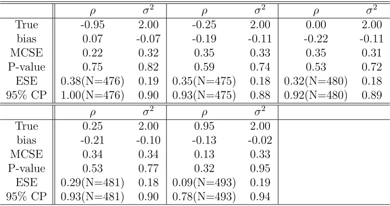
1.4.1 Results based on ML estimates

The main results from the simulation are summarized numerically by using

ta-bles and graphically by using figures. First, from the Table 1.1, notice that there

are few missing estimates of the estimated standard errors (ESE) based on the

ob-served Fisher information matrix. This is due to the fact thatRhas a functionderiv

that numerically computes the derivative of complicated expressions which can lead

(36)

Fisher information is used for the estimation of the Fisher information with the

sec-ond derivative of the log-likelihood function.

From the Table 1.1, we observe that for all cases the estimated values are not

sig-nificantly different from the true value at 5% level. In other words, for all five choices

of ρ, there are no significant biases (all p-values are bigger than 0.32). Asymptotic

variance (ESE’s) of ρ is a good approximation to finite sample variance when the

spatial dependence is weak such as in Cases 2,3, and 4, because the ESE’s are close to

MCSE’s. For Case 1, with 476 estimated variances for ρ, ESE=0.38 and the nominal

95% CP is away from 0.95. In this case, MLE tends to estimate the true value with

high uncertainty. From the Figures in Appendix A.4.1, we observe out that the

esti-mates ofρ’s for boundary values are skewed to right and left for the negative extreme

value and the positive extreme value, respectively (Case 1 and Case 5). But for Cases

2,3, and 4 of ρ, the histograms are appear symmetric.

For all cases, the biases of MLE’s of σ2 _{tend to be negative. However, those}

negative biases are not significant at 5% level. Furthermore, asymptotic variances

(ESE’s) are almost half of MCSE’s suggesting that asymptotic s.e.’s of σ2 _generally

underestimate the finite sample uncertainty. In this cases, MLE’s of σ2_{’s are}

rea-sonable estimates even though there seems to be some degree of underestimation.

From the figures in Appendix A.4.1, we observe that the histogram of MLE’s of σ2

is almost symmetric except for some small values. Therefore, the MLE’s of σ2 _agree

quite closely to the large sample Gaussian approximation.

For the estimation ofβ’s, the estimates did not display significant bias with small

(37)

Table 1.1: Performance of MLE’s of ρ’s and σ2_’s

ρ σ2 _ρ _σ2 _ρ _σ2

True -0.95 2.00 -0.25 2.00 0.00 2.00

bias 0.07 -0.07 -0.19 -0.11 -0.22 -0.11

MCSE 0.22 0.32 0.35 0.33 0.35 0.31

P-value 0.75 0.82 0.59 0.74 0.53 0.72

ESE 0.38(N=476) 0.19 0.35(N=475) 0.18 0.32(N=480) 0.18 95% CP 1.00(N=476) 0.90 0.93(N=475) 0.88 0.92(N=480) 0.89

ρ σ2 _ρ _σ2

True 0.25 2.00 0.95 2.00

bias -0.21 -0.10 -0.13 -0.02

MCSE 0.34 0.34 0.13 0.33

P-value 0.53 0.77 0.32 0.95

ESE 0.29(N=481) 0.18 0.09(N=493) 0.19 95% CP 0.93(N=481) 0.90 0.78(N=493) 0.94

the histograms of estimates displayed in Appendix (Figures A.2 through A.6), we

observe that the finite sample performance of MLE’s of β’s are close to the large

sample Gaussian approximation.

1.4.2 Results based on Bayes estimates

For this simulation study using a Bayesian method, we repeat only 10 times

(N = 10) for sample generation and for the estimation, because it is time consuming

to run more Monte Carlo runs involving MCMC methods. As we discussed in

Sec-tion 1.3.2, the posterior median is considered as Bayes estimates because it provides

more robust estimate than the posterior mean. Also, for an interval estimate of the

parameter, we consider a 95% equal tail credible set (CS) of the sampled values.

From the Table 1.2, we observe that for all estimated parameters, p-values are

(38)

estimates. For all cases, the biases ofρ are slightly positive, but these are not

signifi-cant (all p-values are bigger than 0.18). For Case 2, the nominal 95% CP is away from

0.95 indicating that Bayesian estimation tends to estimate the true value with high

uncertainty. For Case 5, bias is small and MCSE is smaller than any other cases with

1.00 of the nominal 95% CP. Thus, Bayesian estimation tends to estimate the true

value quite well when the true value of ρ is in positive boundary. From the Figures

in Appendix A.4.2, we find out that the posterior distribution of ρ’s for boundary

values are skewed to right and left for Case1 and Case 5, respectively. But for Cases

2,3, and 4 of ρ, the posterior distributions are quite symmetric.

For all cases except Case 1, the biases of Bayesian estimates of σ2 _{tend to be}

positive. This result is a bit different compared to that of MLE’s, because the biases

of MLE’s of σ2 _{tend to be negative for all cases. However, biases of all cases are not}

significant because all p-values are bigger than 0.5 for the Bayesian estimates of σ2_.

The nominal 95% CP’s are quite high for all cases which might be an artifact that

N = 10 only. From the figures in Appendix A.4.2, we observe that the posterior

distribution of σ2 _{is almost symmetric except some small values.}

For the estimation ofβ’s, the estimates do not display significant bias at 5% level.

For Case 1,2 3 and 4, small MCSE are observed with quite high 95% CP’s. However,

for Case 5, MCSE of β0 is much bigger than any other cases with 1 of 95% CP’s.

Thus, in this case, Bayesian estimate of β0 tends to estimate the true value with

high uncertainty. From the posterior distribution displayed in Appendix (Figures A.7

through A.11), we observe that posterior distribution ofβ’s are symmetric. However,

(39)

Table 1.2: Performance of Bayesian estimates of ρ’s and σ2_’s

ρ σ2 _ρ _σ2 _ρ _σ2

True -0.95 2.00 -0.25 2.00 0.00 2.00 bias 0.15 -0.06 0.02 0.03 0.33 0.08 MCSE 0.19 0.12 0.29 0.24 0.48 0.22 P-value 0.43 0.62 0.95 0.90 0.49 0.72 95% CP 0.80 1.00 1.00 0.90 0.70 0.90

ρ σ2 _ρ _σ2

True 0.25 2.00 0.95 2.00 bias 0.01 0.06 0.04 0.10

MCSE 0.43 0.31 0.03 0.15

P-value 0.98 0.85 0.18 0.50 95% CP 0.90 0.70 1.00 1.00

1.5 Extensions of CAR model

Gaussian CAR models have been used as random effects within generalized mixed

effects models to explain the effect of neighbors. As we discussed above, Gaussian

CAR model has merits that the joint distribution is multivariate Gaussian. So, the

ML and the Bayesian estimations are easily obtained. One limitation of the CAR

model is that it assumes that the effects of neighbors are the same in any direction.

However, the magnitude of autocorrelation might be different for different directions.

Thus, there is need to extend a regular CAR model to a new CAR model that

cap-tures spatial anisotropy. We will call this new model as directional CAR (DCAR)

model and is described in Chapter 2. In Chapter 3, we provide a further

general-ization of the DCAR model which determines the neighborhoods adaptively using

a smooth function of the inter-distances and inter-angles between the regions. We

will call this model as the generalized CAR (GCAR) model. We derive the ML

(40)

we establish consistency and asymptotic normality of the MLE’s for DCAR model

under mild regularity conditions. In order to validate the finite sample performance

of the MLE’s and Bayes estimates, we conduct a thorough simulation study in both

Chapters 2 and 3. Finally, real data sets are used to illustrate the implementation of

the proposed methodologies. Additional results are presented in an extended version

(41)

Chapter 2 Directional CAR models

In a regular CAR model, we assume that the conditional effects of neighbors are

the same in any direction which is captured by the spatial effect parameter ρ. In

this chapter, we develop an extension of a regular CAR model using different weights

for different directions. In other words, different weights are given to neighbors in

different directions. We call this model as the directional CAR (DCAR) model.

In general, as we discussed in Chapter 1, we usually consider the model for the

aggregated responses as

Yi =µi+ηi+ǫi (2.1)

whereµi’s denote large-scale variations,ηi represents small-scale variations (or spatial

random effects) and ǫi represents iid measurement errors. We discussed details about

this model in the previous chapter and we note that it is often easier to assume a

spatial latent process, Z = (Z1, . . . , Zn), where Zi = Z(Si) = µi +ηi, and then to

construct models with the moments ofY = (Y1, . . . , Yn). In Chapter 1, a regular CAR

(42)

a regular omni-directional CAR model, we consider the DCAR model to model the

spatial autocorrelation.

2.1 Directional CAR models

In order to model the latent spatial process Zi’s with a DCAR model, first, we

need to consider how to define neighbor structure that depends on the directions

from a centroid of each sub-regions. For illustrations and notation simplicity assume

that Si are regions in a two-dimensional space, i.e., Si ⊂R2_, _∀_i._{However, the model}

and associated statistical inference presented in this thesis can easily be extended to

higher dimensional data. Let si = (s1i, s2i) be a centroid of the sub-region Si, where

s1i corresponds to the horizontal coordinate (x-coordinate) ands2i corresponds to the

vertical coordinate (y-coordinate). The angle (in radian) betweenSi andSj is defined

as

αij =α(Si, Sj) =

  

tan−1₍s2j−s2i

s1j−s1i)

if s2j −s2i ≥0

− π−tan−1₍s2j−s2i

s1j−s1i)

if s2j −s2i <0

for all j 6=i. We consider directions of neighbors from the centroid of subregionSi’s. For example, in Figure 2.1,Sj is in the north-east region of Si and henceα(Si, Sj) is

in [0,π₂). Let Ni represents a set of indexes of neighborhoods for the i-th region Si

(43)

S_i S_j

alpha(S_i,S_j)

Figure 2.1: The angle (in radian) αij

can now create new sub-regions, for each i, as follows:

Ni1 = {j :j ∈ Ni,0≤αij < π

2}, Ni2 = {j :j ∈ Ni,

π

2 ≤αij < π}, Ni3 = {j :j ∈ Ni, π≤αij <

3 2π}, Ni4 = {j :j ∈ Ni,

3

2π ≤αij <2π}.

In a regular CAR model, Ni were chosen to form a clique for i= 1, . . . , n. However,

if j ∈ Ni1 then we should ensure that i ∈ Nj3. For the above set of four

sub-neighborhoods, we can combine each pair of the diagonally opposite neighborhoods

to form a new neighborhood, i.e., we can createN∗

i1 =Ni1SNi3, andNi2∗ =Ni2SNi4

for i = 1, . . . , n. Now it is easy to check that if j ∈ N∗

i1, then i ∈ Nj1∗. Thus, we

redefine two subsets of Ni’s as follows:

N_i1∗ = {j :j ∈ Ni and (0≤αij < π

2 orπ ≤αij < 3 2π)}

N_i2∗ = {j :j ∈ Ni and ( π

2 ≤αij < π or 3

2π ≤αij <2π)}. (2.2) Then, each ofN∗

i1 andNi2∗ forms a clique and thatNi =Ni1∗

S

N∗

i2. The above scheme

of creating new neighborhoods based on the inter-angles,αij’s can be extended beyond

(44)

But for the rest of the article we restrict our attention to case with only two

sub-neighborhoods as described in (2.2).

Based on subsets of the associated neighborhoods, N∗

i1 and Ni2∗, we can construct

directional weight matrices W(1) _{= ((}_w(1)

ij )) and W(2) = ((w (2)

ij )), respectively. For

instance, we can define the directional proximity matrices as w(1)_ij = 1 if j ∈ N∗

i1 and

w(2)_ij = 1 if j ∈ N∗

i2. Notice that W = W(1) +W(2) reproduces the commonly used

proximity matrix based on distances as in a regular CAR model defined in Section

1.2.

Now, we construct a regular DCAR model for the latent spatial processZi’s. Like

a regular CAR model, generally we can model the latent spatial DCAR process using

E[Zi|Zj =zjj 6=i,Xi] = µ(Xi,β) + n

X

j=1

c(1)_ij zj −Xjβ

+

n

X

j=1

c(2)_ij zj−Xjβ

Var[Zi|Zj =zjj 6=i,Xi] = σi2

for i = 1, . . . , n, the c(k)_ij denote directional spatial dependence parameters that are

nonzero only if j ∈ N∗

ik and c

(k)

ii = 0 for k = 1,2. Here, for the large-scale trend,

without loss of generality we assume µi =Xiβ whereX is an arbitrary matrix andβ

is a vector of large-scale parameters like what we considered in previous chapter. As

we discussed in Section 1.1, we construct a DCAR model with the lower dimensional

conditional distributions . For ease of estimation and inference, we reduce the number

of spatial dependent parameters through the use of a parametric modelc(k)_ij =δkw(k)ij

with directional spatial parametersδ1 andδ2, and directional proximity matricesW(1)

and W(2) _where_w(k)

ij ≥0 and w (k)

ii = 0 fork = 1,2. Also, because W=W(1)+W(2),

we can reduce the number of conditional variances by assuming σ2

i = σ

2

mi where

(45)

Therefore, we model conditional distribution of directional CAR model for the latent

spatial process Zi with spatial parameterδ = (δ1, δ2) using

E[Zi|Zj =zjj 6=i,Xi] = Xiβ+δ1 n

X

j=1

w_ij(1) zj −Xjβ

+δ2 n

X

j=1

w_ij(2) zj −Xjβ

Var[Zi|Zj =zjj 6=i,Xi] = σ2

mi, (2.3)

for i = 1, . . . , n. As in a regular CAR model we assume that ηi’s do not depend on

X.

The joint distribution based on a given set of full conditional distributions can be

derived using the Brook’s Lemma(Brook, 1964), provided the positivity condition is

satisfied. For the DCAR model, by construction it follows that each of N∗

i1 and Ni2∗

defined in (2.2) forms a clique fori= 1, . . . , n. Thus, it follows from the

Hammersley-Clifford Theorem that the latent spatial process Zi of a DCAR model exists and is a

Markov Random Field (MRF). We now derive the exact joint distribution of theZi’s

by assuming that each of the full conditional distribution is a Gaussian distribution.

2.2 Gaussian DCAR models

The Gaussian CAR model has been used widely for the latent spatial process

Zi as we discussed in Section 1.2. In this section, we study merits of the Gaussian

DCAR model. As we discussed in previous section, the joint distribution can be easily

derived from the conditional distributions by using Brook’s Lemma.

Assume that the full conditional distributions of Zi’s are given as

Zi|Zj =zj, j 6=i,xi ∼N

xT

i β+

2

X

k=1 δk

n

X

j=1

w_ij(k) zj−xTjβ

, σ 2

mi

(46)

where w(k)_ij for k = 1,2 are the directional weights. It can be shown that this latent

spatial DCAR process Zi’s is a MRF. Thus, by Brook’s lemma and the

Hammersley-Clifford Theorem, it follows that the finite dimensional joint distribution is a

multi-variate Gaussian distribution given by

Z ∼Nn Xβ, σ2(I−δ1W(1)−δ2W(2))−1D

, (2.5)

where Z = (Z1, . . . , Zn)T _and _D _{= diag(} 1 m1, . . . ,

1

mn). For simplicity, we denote the

variance-covariance matrix of DCAR process by Σ∗_Z ≡σ2₍_I₋_δ1_W(1)₋_δ2_W(2)₎−1_D_.

For a proper Gaussian model, the variance-covariance matrixΣ∗_Z is required to be positive definite. If we use the standardized directional proximity matrices ˜W(k) ₌

(( ˜w_ij(k)= w

(k)

ij

mi )), k= 1,2, it can be easily shown that Σ ∗

Z is symmetric.

Next, we derive a sufficient condition that ensures that the variance-covariance

matrix Σ∗_Z is non-singular. As D is a diagonal matrix, we only require suitable conditions on ˜W(k) _{and on}_δk _for _k _{= 1}_,_{2. The following results provides a sufficient}

condition:

Lemma 2 Let A = I− PK_k=1δkW˜ (k) _{be an} _n _×_n _{matrix where} PK

k=1W˜ (k) is a

symmetric matrix with non-negative entries, diagonal 0 and each row sums to unity.

If max1≤k≤K|δk|<1, then the matrix A is positive definite.

Proof: Let aij denote the (i, j)-th element of A. Notice that for each i= 1,2. . . , n,

we have

X

j6=i

|aij|=X

j6=i

|

K

X

k=1

δkw(k)_ij | ≤

K

X

k=1

|δk|X

j6=i

w(k)_ij < K

X

k=1

X

j6=i

w(k)_ij = 1 =aii

Hence it follows from Lemma 3 that A is positive definite. Based on Lemma 2

Generalized Conditionally Autoregressive Models

ABSTRACT

Biography

Acknowledgements

Contents

List of Tables

List of Figures

Chapter 1

Introduction to Conditionally

Autoregressive Models

1.1

Markov Random Field

1.2

Gaussian CAR models

1.3

Parameter estimation

1.3.1

Maximum likelihood estimation

1.3.2

Bayesian estimation

1.4

A simulation study

1.4.1

Results based on ML estimates

1.4.2

Results based on Bayes estimates

1.5

Extensions of CAR model

Chapter 2

Directional CAR models

2.1

Directional CAR models

2.2

Gaussian DCAR models