Volume 1, No. 2, July‐August 2010
International
Journal
of
Advanced
Research
in
Computer
Science
RESEARCH
PAPER
Available Online at www.ijarcs.info
Predictability of Software Reliability With Imperfect Debugging Based on Multiple
Change Point
O. NagaRaju * Asst. Professor
Acharya Nagarjuna University Nagarjuna Nagar, INDIA
Dr. R. SatyaPrasad Associate Professor Acharya Nagarjuna University
Nagarjuna Nagar, INDIA [email protected] Prof. R. R. LKantam
Professor Nagarjuna University Nagarjuna Nagar, INDIA [email protected]
Abstract:In this paper, we propose to investigate some techniques for predictability of software reliability with imperfect debugging. And we
also incorporate the concept of multiple change points in SRGM. Some models are proposed and discussed under both ideal and imperfect debugging conditions. A numerical example with real software failure data is presented in detail and the results show that the proposed models can provide better capability to predict the software reliability.
Keywords: Non homogeneous poisson process, software reliability, imperfect debugging, failure data.
I. INTRODUCTION
Several distinct faces of engineering a software are de-finition ,analysis, development, text and maintenance etc., A very important role is developed by software reliability measurement as a robust, high quality software product be-tween software reliability and assured software quality, as applied by software reliability growth model (SRGM) Gen-eral formulation can unify various traditional SRGMs. Generally, at the beginning of the testing phase, inspection can discover many faults and the fault discovery efficiency depends on the fault detection rate, the fault density, the testing-effort and the inspection rate.
The change point problem in the field of soft reliability has been addressed by some papers in recent years. Differ-ent assumptions are made in differDiffer-ent SRGMs. Therefore problem of imperfect debugging can be applied to different situations as addressed by many authors.
However, this may not be correct since the testing envi-ronment may not reproduce the typical use of the system in field operation [4, 10, and 15]. The fault detection phe-nomenon in the operational phase is different from that in the testing phase. Thus we have to make an adjustment for the selected SRGM that was accurate in the past. Here we will further propose a very useful approach to describe the transitions from the testing to the operational phase. That is, based on the unified theory, we can incorporate the concept of multiple change-points into software reliability modeling. Besides, the proposed models are also discussed under both ideal and imperfect debugging conditions.
II. SOFTWAREOPERATIONAL RELIABILITY MEASUREMENT
A. A General Continuous SRGM
We will discuss a general continuous NHPP model in this section. We let m(t+Δt) be equal to the quasi-arithmetic mean of m(t) and a with weights w(t, Δt) and 1-ω(t, Δt), then
1
)
,
(
0
),
(
))
,
(
1
(
))
(
(
)
,
(
))
(
(
m
t
+
Δ
t
=
t
Δ
t
g
m
t
+
−
t
Δ
t
g
a
<
t
Δ
t
<
g
ω
ω
ω
………. (2.1)
Where g is a real-valued, strictly monotonic, and differenti-able function.
))),
(
(
)
(
(
)
,
(
1
))
(
(
))
(
(
t
m
g
a
g
t
t
t
t
t
m
g
t
t
m
g
−
Δ
Δ
−
=
Δ
−
Δ
+
ω
0<ω(t,Δt)<1.
Suppose (1- ω(t, Δt)/ ΔtÆb(t) as ΔtÆ0, we get the differen-tial equation
)).
(
(
)
(
)
(
))
(
(
m
t
b
t
g
a
g
m
t
g
t
=
−
∂
∂
…………. (2.2) For g(x)=x in equation, then
)).
(
)(
(
))
(
(
m
t
b
t
a
m
t
g
t
=
−
∂
∂
………. (2.3) Here, b(t) is the fault detection rate per error. Furthermore, if b(t)=b then if would be the popular SRGM of Goel-Okumoto model(1979)in short known as G-O model.
Theorem: let
))),.
(
(
)
(
)(
(
))
(
(
m
t
b
t
g
a
g
m
t
g
t
=
−
∂
∂
where g is a real-valued, strictly monotonic, and differenti-able function. We have:
m
t
g
g
a
{
g
m
g
a
}
e
a
b
⎟⎠t
⎞ ⎜
⎝ ⎛
−
+
−
+
=
(
(
)
(
(
0
)
(
)
β
)
(
1and
∫
=
t
du
u
a
t
B
0
)
(
)
(
Corollary1: Based on the weighted arithmetic mean, take g(x)=x in equation and let k=1-m(0)/a, then the mean value function, Our proposed mean value function for the model with the above specification is
⎪
⎪
⎭
⎪⎪
⎬
⎫
⎪
⎪
⎩
⎪⎪
⎨
⎧
−
+
+
⎥
⎥
⎥
⎥
⎦
⎤
⎢
⎢
⎢
⎢
⎣
⎡
+
+
+
−
=
⎟ ⎠ ⎞ ⎜
⎝ ⎛
⎟ ⎠ ⎞ ⎜
⎝ ⎛
β
β
β
β
β
β
1 1
1
1
(
)
1
1
2
1
)
(
a
b
a
b
t
b
a
ke
b
a
t
b
a
ke
b
a
t
m
, a>0, 0<k≤1…………. (2.5)
B. Software Operational Reliability Estimation Based on Multiple Change-Point SRGMs
⎪
⎪
⎭
⎪⎪
⎬
⎫
⎪
⎪
⎩
⎪⎪
⎨
⎧
−
+
+
⎥
⎥
⎥
⎥
⎦
⎤
⎢
⎢
⎢
⎢
⎣
⎡
+
+
+
−
=
⎟ ⎠ ⎞ ⎜
⎝ ⎛
⎟ ⎠ ⎞ ⎜
⎝ ⎛
β
β
β
β
β
β
1 1
1 1
1
(
)
1
1
2
1
)
(
a
b
a
b
t
b
a
e
b
a
t
b
a
e
b
a
t
m
In reality, the fault detection phenomenon in the opera-tional phase is different from that in the testing phase [7, 16, 17, 19-22]. However, this fact is not distinctly incorporated in many software reliability modeling efforts. Generally, at the beginning of the testing phase, many faults can be dis-covered by inspection and the fault detection rate depends on the fault discovery efficiency, the fault density, the test-ing-effort, and the inspection rate. In the middle stage of testing phase, the fault detection rate normally depends on other parameters such as the execution rate of CPU instruc-tion, the code expansion factor, and the scheduled CPU hours per calendar day. Consequently, the fault detection rate can be calculated. We can use this rate to track the pro-gress of checking activities, to evaluate the effectiveness of test planning, and to assess the checking methods we adopted. Practically, during the software development proc-ess, the fault detection rate may not be a constant or smooth, i.e., it may be changed at some time moment called change-point.
In general, a change-point is a model which has some parameters which are discontinuous in time. That is, it is the time at which the parameter changes its values. In the recent years, some papers have addressed the change-point [2, 5, 11, and 13].If we want to detect more additional faults dur-ing software development process; it is advisable to intro-duce new tools and techniques. That is these approaches can provide a steady improvement in software testing and pro-ductivity. Therefore, the timing of introducing new tools and techniques is a change-point. In this paper, we will show how to improve traditional SRGMs by incorporating the concepts of multiple change points.
C. Our Model with Multiple Change-Points
The G-o model mathematical expression can be ex-pressed as
))
(
(
)
(
t
m
a
b
t
t
m
−
=
∂
∂
……… (2.6)
Solving above equations using the boundary conditions m(0)=0, we have m(t)=a(1-exp[-bt]) and
(
)
b
(
t
)[
a
m
(
t
)]
t
t
m
−
=
∂
∂
……….. (2.7) On the same lines we propose our model as
⎪
⎪
⎭
⎪⎪
⎬
⎫
⎪
⎪
⎩
⎪⎪
⎨
⎧
−
+
+
⎥
⎥
⎥
⎥
⎦
⎤
⎢
⎢
⎢
⎢
⎣
⎡
+
+
+
−
=
⎟ ⎠ ⎞ ⎜
⎝ ⎛
⎟ ⎠ ⎞ ⎜
⎝ ⎛
β
β
β
β
β
β
1 1
1
1
(
)
1
1
2
1
)
(
a
b
a
b
t
b
a
e
b
a
t
b
a
e
b
a
t
m
……… (2.8)
Further the model with two change points and a given the fault deletion rate as given by
b(t) =
a
1 if 0≤t≤τ
1b(t) =
a
2 if t>τ
solving similar equations. The solutions are , 0≤t≤
τ
1………..(2.9)⎪ ⎪ ⎭ ⎪⎪ ⎬ ⎫
⎪ ⎪ ⎩ ⎪⎪ ⎨ ⎧
− + + ⎥ ⎥ ⎥ ⎥
⎦ ⎤
⎢ ⎢ ⎢ ⎢
⎣ ⎡
+ − =
− + +
− + +
β β
β β
τ τ
β
τ τ
β
1 1
1
1 ( )
1 1 2 1 ) (
)) 1 ( 2 1 1 (
)) 1 ( 2 1 1 (
1 2
b a b a
b a
b a
t m
t t a a a e
t t a a a e
, t>
τ
……….. (2.10)In fact, the above equation can also be derived based on the unified theory, but we have to make some necessary adjustments for Theorem due to multiple change points. Firstly, when0≤t≤
τ
1,if we take g(x)=x,k1-m(0)/a, andBB1(t)= from the corollary1, we can easily obtain the mean value function m
du
a
∫
τ0 1
1(t)=a(1-exp[-b1t]) furthermore, when
t>τ, if we take g(x)=x and B2(t)= , then from the
corollary 1, we have
du
a
∫
τ0 2
⎪
⎪
⎭
⎪⎪
⎬
⎫
⎪
⎪
⎩
⎪⎪
⎨
⎧
−
+
+
⎥
⎥
⎥
⎥
⎦
⎤
⎢
⎢
⎢
⎢
⎣
⎡
+
−
=
− + +
− + +
β
β
β
β
τ
τ
β
τ
τ
β
1 1
1
1
(
)
1
1
2
1
)
(
)) 1 ( 2 1 1 (
)) 1 ( 2 1 1 (
2
b
a
b
a
b
a
b
a
t
m
t t a a a e
t t a a a e
If e a a t
a
m
k
2=
1
−
1(
τ
)
=
(β
+ 1τ
1)we obtain
⎪
⎪
⎭
⎪⎪
⎬
⎫
⎪
⎪
⎩
⎪⎪
⎨
⎧
−
+
+
⎥
⎥
⎥
⎥
⎦
⎤
⎢
⎢
⎢
⎢
⎣
⎡
+
−
=
− + +
− + +
β
β
β
β
τ
τ
β
τ
τ
β
1 1
1
1
(
)
1
1
2
1
)
(
)) 1 ( 2 1 1 (
)) 1 ( 2 1 1 (
2
b
a
b
a
b
a
b
a
t
m
t t a a a e
t t a a a e
a
1 if 0≤t≤τ1 b(t)=a
2 if τ1≤t≤τ2…..
a
n if τn-1≤t≤τn
The mean value function can be obtained by following simi-lar procedures. These are
⎪
⎪
⎭
⎪⎪
⎬
⎫
⎪
⎪
⎩
⎪⎪
⎨
⎧
−
+
+
⎥
⎥
⎥
⎦
⎤
⎢
⎢
⎢
⎣
⎡
+
−
=
=
+ +β
β
β
β
β
β
1 1 1 11
(
)
1
1
2
1
)
(
)
(
) ( ) (b
a
b
a
b
a
b
a
t
m
t
m
t b a e t b a e0≤t≤τ1……….. (2.12)
⎪
⎪
⎭
⎪⎪
⎬
⎫
⎪
⎪
⎩
⎪⎪
⎨
⎧
−
+
+
⎥
⎥
⎥
⎥
⎦
⎤
⎢
⎢
⎢
⎢
⎣
⎡
+
−
=
=
− + + − + +β
β
β
β
τ
τ
β
τ
τ
β
1 1 1 12
(
)
1
1
2
1
)
(
)
(
)) 1 ( 2 1 1 ( )) 1 ( 2 1 1 (b
a
b
a
b
a
b
a
t
m
t
m
t t a a a e t t a a a eτ1≤t ≤τ2………. (2.13)
⎪ ⎪ ⎭ ⎪⎪ ⎬ ⎫ ⎪ ⎪ ⎩ ⎪⎪ ⎨ ⎧ − + + ⎥ ⎥ ⎥ ⎥ ⎦ ⎤ ⎢ ⎢ ⎢ ⎢ ⎣ ⎡ + − = = − + − + + − + − + + β β β β τ τ τ τ β τ τ τ τ β 1 1 3 3 2 1 1 1 3 3 2 1 1 1
3 ( )
1 1 2 1 ) ( ) ( ) ( ) 1 2 ( ( ) ( ) 1 2 ( ( b a b a b a b a t m t m t t a a a a e t t a a a a e . (2.14) Finally if
a1 if 0 ≤ t ≤τ1
a2 if τ1 ≤ t ≤τ2
b(t) = ….
an if τn-1 ≤ t ≤τn
and
(
1)
1
1 1
)
(
1
1
− −− = −
∑
=
−
−
=
n k kk k n n n
a
a
m
k
τ
τ
τ
we can get a solutions for descending multiple change-points of our model
⎪ ⎪ ⎪ ⎪ ⎭ ⎪⎪ ⎪ ⎪ ⎬ ⎫ ⎪ ⎪ ⎪ ⎪ ⎩ ⎪⎪ ⎪ ⎪ ⎨ ⎧ − + ⎟⎟ ⎠ ⎞ ⎜⎜ ⎝ ⎛ + ⎥ ⎥ ⎥ ⎥ ⎥ ⎥ ⎥ ⎥ ⎦ ⎤ ⎢ ⎢ ⎢ ⎢ ⎢ ⎢ ⎢ ⎢ ⎣ ⎡ ∑− = − − + − − + + ∑− = − − + − − + − = ⎟⎟ ⎟ ⎟ ⎟ ⎠ ⎞ ⎜⎜ ⎜ ⎜ ⎜ ⎝ ⎛ ⎪ ⎪ ⎭ ⎪⎪ ⎬ ⎫ ⎪ ⎪ ⎩ ⎪⎪ ⎨ ⎧ ⎟⎟ ⎟ ⎟ ⎟ ⎠ ⎞ ⎜⎜ ⎜ ⎜ ⎜ ⎝ ⎛ ⎪ ⎪ ⎭ ⎪⎪ ⎬ ⎫ ⎪ ⎪ ⎩ ⎪⎪ ⎨ ⎧ β β τ τ τ β β τ τ τ β β 1 1 1 1 1
1 *( 1) ) 1 ( * 1 1 1 ) 1 ( * ) 1 ( * 1 2 1 )
( a b a b
t n k a t a a e b a t n k a t a a e b a t m k k k n n k k k n n n (2.15)
D. Generalization of our Model with Multiple Change Point:
We can follow similar procedure described to the general-ized model with multiple change mends
If bk(t) = akctc-1
We can get the mean value functions
⎪ ⎪ ⎪ ⎪ ⎭ ⎪⎪ ⎪ ⎪ ⎬ ⎫ ⎪ ⎪ ⎪ ⎪ ⎩ ⎪⎪ ⎪ ⎪ ⎨ ⎧ − + ⎟⎟ ⎠ ⎞ ⎜⎜ ⎝ ⎛ + ⎥ ⎥ ⎥ ⎥ ⎥ ⎥ ⎥ ⎥ ⎦ ⎤ ⎢ ⎢ ⎢ ⎢ ⎢ ⎢ ⎢ ⎢ ⎣ ⎡ ∑− = − + − + + − ∑− = − + − + + − = ⎪ ⎪ ⎭ ⎪⎪ ⎬ ⎫ ⎪ ⎪ ⎩ ⎪⎪ ⎨ ⎧ − − ⎪ ⎪ ⎭ ⎪⎪ ⎬ ⎫ ⎪ ⎪ ⎩ ⎪⎪ ⎨ ⎧ − − β β τ τ τ β β τ τ τ β β 1 1 1 1 1 1 1 1 1
1*( )
) ( 1 1 1 ) ( * ) ( 1 2 1 )
( a b a b
t n k a c c t a a e b a t n k a c c t a a e b a t m c k c k k n n c k c k k n n n c c ...(2.16)
III. IMPERFECT-DEBUGGING MODELING
In general, different SRGM make different assumptions and therefore can be applied to different situations. From
our studies, most SRGMs assume that each time a failure occurs, that fault that caused it is immediately removed and no new faults are introduced sometimes these assumptions can help to reduce the complaints of modeling software reli-ability[8,12]. As we know that software debugging is the process of identifying the cause for software detective be-havior and addressing that problem, there is much this paper can address the problem of imperfect debugging [6, 18]. We plan to incorporate relaxations of some assumptions in order to make the SRGMs more realistic and practical.
A general continues SRGM we let m(t+Δt) be equal to the quasi arithmetic mean of m(t) and a with weights w(t,Δt) and 1-w(t,Δt), then:
(m(t+Δt))= G(m(t,Δt) g(m(t)+(1-w(t,Δt))g(a),0<w(t,Δt)<1. Where g is real-valued by modifying equations (A) if we let m(t+Δt) be equal to the quasi arithmetic mean of m(t) and n(t) with weights w(t,Δt) and 1-w(t,Δt) then:
g(m(t+Δt)) = w(t,Δt) g(m(t))+(1-w(t,Δt))g(n(t))
Where n(t) is the fault content functions (n(0)=a) g is a real – valued; strictly monotonic and differentiable function. That is
))
(
(
)
(
(
(
)
,
(
1
))
(
(
))
g(m(t
t
m
g
t
n
g
t
t
t
w
t
t
m
g
t
−
Δ
Δ
−
=
Δ
−
Δ
……….(3.1)Suppose (1-w(t,Δt))/Δt b(t) as Δt 0, we get the differential equations.
(
g
(
m
(
t
))
b
(
t
){
g
(
n
(
t
))
g
(
m
(
t
))}
t
=
−
∂
∂
.. (3.2) For example if g(x) =x from (3.2) becomes
)}
(
)
(
){
(
))
(
(
(
g
m
t
b
t
n
t
m
t
t
=
−
∂
∂
……….(3.3) The following theorem is true
Let
(
g
(
m
(
t
))
b
(
t
)
g
(
n
(
t
))
g
(
m
(
t
))
t
=
−
∂
∂
Where G is a real valued, strictly monotonic, and differ-entiable function we have
)
exp
))}
(
(
)
0
(
(
{
))
(
(
(
)
(
1 [(a b)t]t
n
g
m
g
t
n
g
g
t
m
=
−+
−
β+and
∫
=
tdu
u
a
t
B
0)
(
)
(
A. Our Model with Multiple Change Points and Imperfect Debugging
We can describe our model with single change point under imperfect debugging as the following
))
(
(
*
)
(
)
(
t
m
a
t
b
t
t
m
=
−
∂
∂
We can get the resulting the model is
))
(
)
(
(
*
)
(
)
(
t
m
t
n
t
b
t
t
m
=
−
∂
∂
……… (3.4) and b1=a1(t) if 0≤t≤τ
Here we note that n(t) is a fault content function which is defined as the sum of the expected number of initial soft-ware faults are introduce d faults as a function f time ‘t’. There are some fault content functions in (3.4), but further discussion of this is beyond the scope of this paper there we assume:
t
t
m
t
t
m
∂
∂
=
∂
∂
(
)
β
(
)
………. (3.5)
Where β is the fault introductions rate and n (0) =a. Therefore eq (2) becomes
N(t)=βm(t)+c N(0)=βm(0)+c A=0+c
Therefore n(t)=βm(t)+c
)]
(
)[
(
)
(
t
m
a
t
b
t
t
m
β
+
=
∂
∂
……….. (3.6)Solving eq(3.6) and assuming m(0)=0 we obtain the mean value function as follows
[
(
)
(
)
]
)
(
)
(
t
m
t
m
a
t
b
t
t
m
−
+
=
∂
∂
β
[
(
)(
1
)
]
)
(
)
(
=
+
−
∂
∂
β
t
m
a
t
b
t
t
m
⎪ ⎪ ⎭ ⎪⎪ ⎬ ⎫ ⎪ ⎪ ⎩ ⎪⎪ ⎨ ⎧ − − + ⎟⎟ ⎠ ⎞ ⎜⎜ ⎝ ⎛ − + ⎥ ⎥ ⎥ ⎥ ⎦ ⎤ ⎢ ⎢ ⎢ ⎢ ⎣ ⎡ + − − + + − − − − = β β β β β ββ (1 ) ) 1 1
2 ) 1 ( 1 ) ) 1 ( 2 ) 1 ( 1 ) 1 ( 2 1 )
( 1 1
1 1 b a b a t a a e a t a a e a t m ⎪ ⎪ ⎭ ⎪⎪ ⎬ ⎫ ⎪ ⎪ ⎩ ⎪⎪ ⎨ ⎧ − − + ⎟⎟ ⎠ ⎞ ⎜⎜ ⎝ ⎛ − + ⎥ ⎥ ⎥ ⎥ ⎦ ⎤ ⎢ ⎢ ⎢ ⎢ ⎣ ⎡ − − + + − − + − − + + − − − − = β β τ β τ β β τ β τ β β
β (1 ) ) (1 )( )) 1 1 2 ) 1 ( 1 )) )( 1 ( ) ) 1 ( 2 ) 1 ( 1 ) 1 ( 2
1 1 1
2 1 2 1 b a b a t a a a e a t a a a e a ……. (3.7)
In fact eq(3.7) we can also solve based on the unified theory for SRGM. Finally when 0≤t≤τ, if we take g(x)=x,
a
m
k
1=
1
−
(
1
−
β
)
(
0
)
From theorem, we can easily obtain the mean value func-tions ⎪⎭ ⎪ ⎬ ⎫ ⎪⎩ ⎪ ⎨ ⎧ − − + ⎟⎟ ⎠ ⎞ ⎜⎜ ⎝ ⎛ − + ⎥ ⎥ ⎦ ⎤ ⎢ ⎢ ⎣ ⎡ + − − + + − − − −
= β β β
β β β
β 1 (1 ) (1 ) ) 1 1
) ) 1 ( ) 1 ( 1 ) 1 ( 2 1 )
( 1 1
1 1
1 a b a b
t a a e a t a a e a t m ……….. (3.8)
Furthermore, when t>τ,if we take g(x)=x and B2(t)= a2du
then from theorem we have
⎪⎭ ⎪ ⎬ ⎫ ⎪⎩ ⎪ ⎨ ⎧ − − + ⎟⎟ ⎠ ⎞ ⎜⎜ ⎝ ⎛ − + ⎥ ⎥ ⎦ ⎤ ⎢ ⎢ ⎣ ⎡ − − − + − − − − − = + + β β τ β β τ β β
β 1 (1 ) ( (1 )( )) 1 1
)) )( 1 ( ( ) 1 ( 1 ) 1 ( 2 1 )
( 1 1
2 2
2 2
2 a b a b
t a k e a t a k e a t m …….. (3.9)
Where k2=1-(1-β)m1(τ)=exp (a(1-β)+b11τ
Also the fault contest function is given by
⎪ ⎪ ⎭ ⎪⎪ ⎬ ⎫ ⎪ ⎪ ⎩ ⎪⎪ ⎨ ⎧ − − + ⎟⎟ ⎠ ⎞ ⎜⎜ ⎝ ⎛ − + ⎥ ⎥ ⎥ ⎥ ⎦ ⎤ ⎢ ⎢ ⎢ ⎢ ⎣ ⎡ + − − + + − − − − = = β β β β β β β β
β (1 ) ) 1 1
2 ) 1 ( 1 ) ) 1 ( 2 ) 1 ( 1 ) 1 ( 2 1 ) ( )
( 1 1
2 1
1 a b a b
t a a e a t a a e a t n t n ……….. (3.10) When 0≤t≤τ
When τ<t Finally if
⎥
⎦
⎤
⎢
⎣
⎡
−
−
=
−
−
=
∑
− = − − − 1 1 1 1 1)
(
)
1
(
exp
)
(
)
1
(
1
n k k k n n na
t
m
k
β
β
τ
τ
We obtain a generalized solution for describing the model with multiple change points under suspected debugging.
{ } { } ⎪ ⎪ ⎪ ⎪ ⎭ ⎪ ⎪ ⎪ ⎪ ⎬ ⎫ ⎪ ⎪ ⎪ ⎪ ⎩ ⎪ ⎪ ⎪ ⎪ ⎨ ⎧ − − + ⎟⎟ ⎠ ⎞ ⎜⎜ ⎝ ⎛ − + ⎥ ⎥ ⎥ ⎥ ⎥ ⎦ ⎤ ⎢ ⎢ ⎢ ⎢ ⎢ ⎣ ⎡ ∑ − + ∑ − − − = ⎪⎭ ⎪ ⎬ ⎫ ⎪⎩ ⎪ ⎨ ⎧ + − + − ⎪⎭ ⎪ ⎬ ⎫ ⎪⎩ ⎪ ⎨ ⎧ + − + − − = − − − − = − − − β β β β β τ τ τ β τ τ τ β 1 1 ) 1 ( 1 ) 1 ( 1 ) 1 ( 2 1 ) ( 1 1 [ ) ( ) 1 ( 1 [ ) ( ) 1 ( 1 1 1 ] 1 1 * 1 1 ] 1 1 * b a b a e b a e b a t
m a a t a t
t a t a a n n k k k k n n n k k k k n n and { } { } ⎪ ⎪ ⎭ ⎪ ⎪ ⎬ ⎫ ⎪ ⎪ ⎩ ⎪ ⎪ ⎨ ⎧ − − + ⎟⎟ ⎠ ⎞ ⎜⎜ ⎝ ⎛ − + ⎥ ⎥ ⎥ ⎥ ⎥ ⎦ ⎤ ⎢ ⎢ ⎢ ⎢ ⎢ ⎣ ⎡ ∑ − + ∑ − − − = ⎪⎭ ⎪ ⎬ ⎫ ⎪⎩ ⎪ ⎨ ⎧ + − + − ⎪⎭ ⎪ ⎬ ⎫ ⎪⎩ ⎪ ⎨ ⎧ + − + − − = − − − − = − − − β β β β β β
β β τ ττ
τ τ τ β 1 1 ) 1 ( 1 ) 1 ( 1 ) 1 ( 2 1 )
( 1 1
[ ) ( ) 1 ( 1 [ ) ( ) 1 ( 1 1 1 ] 1 1 * 1 1 ] 1 1 * b a b a e b a e b a t n t a t a a t a t a a n n k k k k n n n k k k k n n ………. (3.11) where τ=0andτn-1<t.
B. Generalized our Model with Multiple Change-Points Considering Imperfect Debugging
The generalized our model with multiple change-points under imperfect debugging, we have the mean value func-tion: { } { } ⎪ ⎪ ⎭ ⎪ ⎪ ⎬ ⎫ ⎪ ⎪ ⎩ ⎪ ⎪ ⎨ ⎧ − − + ⎟⎟ ⎠ ⎞ ⎜⎜ ⎝ ⎛ − + ⎥ ⎥ ⎥ ⎥ ⎥ ⎦ ⎤ ⎢ ⎢ ⎢ ⎢ ⎢ ⎣ ⎡ ∑ − + ∑ − − − = ⎪⎭ ⎪ ⎬ ⎫ ⎪⎩ ⎪ ⎨ ⎧ + − + − ⎪⎭ ⎪ ⎬ ⎫ ⎪⎩ ⎪ ⎨ ⎧ + − + − − = − − − − = − − − β β β β
β β τ τ τ
τ τ τ β 1 1 ) 1 ( 1 ) 1 ( 1 ) 1 ( 2 1 )
( 1 1
[ ) ( ) 1 ( 1 [ ) ( ) 1 ( 1 1 1 ] 1 1 * 1 1 ] 1 1 * b a b a e b a e b a t m n k k c k c k n c c n n k k c k c k n c c n a t a a a t a a n And { } { } ⎪ ⎪ ⎭ ⎪ ⎪ ⎬ ⎫ ⎪ ⎪ ⎩ ⎪ ⎪ ⎨ ⎧ − − + ⎟⎟ ⎠ ⎞ ⎜⎜ ⎝ ⎛ − + ⎥ ⎥ ⎥ ⎥ ⎥ ⎦ ⎤ ⎢⎣ …… (3.12) ⎢ ⎢ ⎢ ⎢ ⎡ ∑ − + ∑ − − − = ⎪⎭ ⎪ ⎬ ⎫ ⎪⎩ ⎪ ⎨ ⎧ + − + − ⎪⎭ ⎪ ⎬ ⎫ ⎪⎩ ⎪ ⎨ ⎧ + − + − − = − − − − = − − − β β β β β β
β β τ τ τ
τ τ τ β 1 1 ) 1 ( 1 ) 1 ( 1 ) 1 ( 2 1 )
( 1 1
[ ) ( ) 1 ( 1 [ ) ( ) 1 ( 1 1 1 ] 1 1 * 1 1 ] 1 1 * b a b a e b a e b a t n n k k c k c k n c c n n k k c k c k n c c n a t a a a t a a n
C. Inflection S-Shaped Model with Multiple Change-Points Considering Imperfect Debugging
The Inflection S-shaped model with multiple change-points under imperfect debugging, we have the mean value function.
β
τ τ
β
τ τ
β
τ τ
β
τ β
ψ β
ψ β
β β ψ
β ψ β
β
−
−
=
⎪ ⎪ ⎪ ⎪ ⎪
⎭ ⎪ ⎪ ⎪ ⎪ ⎪
⎬ ⎫
⎪ ⎪ ⎪ ⎪ ⎪
⎩ ⎪ ⎪ ⎪ ⎪ ⎪
⎨ ⎧
∗ +
∗ −
⎥ ⎥ ⎥ ⎥
⎦ ⎤
⎢ ⎢ ⎢ ⎢
⎣ ⎡
− + + ⎥ ⎥ ⎥ ⎥
⎦ ⎤
⎢ ⎢ ⎢ ⎢
⎣ ⎡
∗ +
∗ −
− =
∏
− − + +
− − + +
− + +
− − +
+ 1
1
1 1 1
1 1
1 1
) 1 ( ) (
) 1 ( ) (
)) 1 ( 2 1 1 (
) 1 ( ) (
1 1
* )
( 1
1
) 1 ( 2
1 ) (
n k n
t n k t n a t k k a a e
t n k t n a t k k a a e
t t a a a e
t n t n a t b a e
b a
b a
b a b a
b a b a
t m
and
β
τ τ
β
τ τ
β
τ τ β
τ β
ψ β
ψ β
β β ψ
β β
ψ β β
β
−
−
=
⎪ ⎪ ⎪ ⎪ ⎪
⎭ ⎪ ⎪ ⎪ ⎪ ⎪
⎬ ⎫
⎪ ⎪ ⎪ ⎪ ⎪
⎩ ⎪ ⎪ ⎪ ⎪ ⎪
⎨ ⎧
∗ +
∗ −
⎥ ⎥ ⎥ ⎥
⎦ ⎤
⎢ ⎢ ⎢ ⎢
⎣ ⎡
− + + ⎥ ⎥ ⎥ ⎥
⎦ ⎤
⎢ ⎢ ⎢ ⎢
⎣ ⎡
∗ − +
∗ − −
− =
∏
− − + +
− − + +
− + +
− − +
+ 1
1
1 1 1
1 1
1 1
) 1 ( ) (
) 1 ( ) (
)) 1 ( 2 1 1 (
) 1 ( ) (
1 1 *
) ( )
1 ( 1
) 1 ( 1
) 1 ( 2
1 ) (
n k n
t n k t n a t k k a a e
t n k t n a t k k a a e
t t a a a e
t n t n a t b a e
b a b a
b a b a
b a b a
t n
… (3.13)
Where
τ
0=0 andτ
n-1<t.Parameter estimations is of primary importance in software reliability predictions. Once the analytical solutions for m (t) are known for a given model, the parameters in the solutions need to be determined. Parameter estimations is achieved by applying a technique of MLE, the most impor-tant and widely used estimation technique. The MLE tech-nique is to estimate the unknown parameters for the soft-ware reliability models.
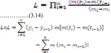
MLE estimates the parameters by following the likeli-hood functions L is
………(3.14)
Differencing the above equations with respect to each unknown parameter and setting the partial derivations to zero yields a set of nonlinear equations .The maximum like-lihood estimations of the parameter can be obtained by solv-ing the set of equations numerically.
The estimate of parameters a and b for specified β using the MLE method can be obtained by solving the following equations simultaneously.
………..(3.15)
……….. (3.16)
⎪ ⎪ ⎭ ⎪⎪ ⎬ ⎫
⎪ ⎪ ⎩ ⎪⎪ ⎨ ⎧
− − + ⎟⎟ ⎠ ⎞ ⎜⎜ ⎝ ⎛
− + ⎥ ⎥ ⎥ ⎥
⎦ ⎤
⎢ ⎢ ⎢ ⎢
⎣ ⎡
− − + + − − +
− − + + − − − − = =
β β τ
β τ β β β
τ β τ β β β
β (1 ) ) (1 )( ) 1 1
2 ) 1 ( 1
) )( 1 ( ) ) 1 ( 2
) 1 ( 1
) 1 ( 2
1 ) ( )
( 1 1
1 2 1
1 2 1
2 a b a b
t a a a e a
t a a a e a
t n t n
D. Numerical Examples
The data used was from the real software project [9].The system was Brazilian electronic switching sys-tem.TROPICOR-1500 for 1500 subscribers. Software size was about 300kb written in assembly language .during 81weeks 461 faults were removed. Actually this data has 81 data entries. Entries 31 through 42 were obtained during field trails, and entries 43 through 81 were obtained during system operation [12]. Here we assume that the 31st week
and the 43rd week as the first and the second change points
[image:5.595.36.229.569.661.2]respectively. The data shows in table1.
Table I: Data of real software project
In order to show quantitative comparisons for long-term predictions, here we use mean square error (MSE) to judge the performance of the model .The MSE can be expressed as.
………….. (3.17)
Where m(ti) is the expected number of faults by time ti
esti-mated by a model ,mi is the observed number of faults by time ti. A smaller MST indicates a smaller tilting error and
better performance.
E. Performance Analysis
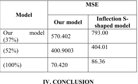
estimated parameters are shown in table2 summarizing the comparisons of the results. Here let’s suppose that the deri-vations of mean value function will take change points into considerations and to estimate software reliability growth. [24]Table 4 the MSE of the unmolded with multiple change points using 52% and 100% results of the data are less than the traditional and model using 52% and 100% of the data in table 3.
[image:6.595.43.274.400.534.2]Finally it is worthwhile to note that by adding more esti-mate parameters in modeling the phenomenon, the estiesti-mates become more difficult as more numerical calculations one involved assume her e additional calculations can be fully automated. Actually if higher reliability is required in same crucial applications the cost of estimate computations for more accuracy is easily justified and is valuable.
Table II: parameter estimations of the our model
a b Ψ
Our Model
(37%) 309.89 0.02009 0.9009 (52%) 450.20 0.0100 0.3400 (100%) 400.90 0.0189 0.2900
[image:6.595.45.273.579.718.2]Table III: comparison results of our model and inflection S-shaped model.
Table IV: Comparison results of our model with multiple change points and inflection S-shaped model.
IV. CONCLUSION
Our model use with and without multiple change point gives smaller MSE in most of situations. Therefore our model as a better predictability of software reliability then the inflection s-shaped model consider by chin-yu huang at 2005 .We proposed several software operational reliability
growth models with multiple change points. We showed that most existing SRGMs and NHPPs can be improved by in-corporating the concepts of multiple change points. We pro-vide a simple but useful approach to measure and access operational software reliability. Our model also discussed under imperfect debugging conditions.
V.REFERENCES
[1] A. L. Goel and K. Okumoto, “An Analysis of Recurrent Software Errors in a Real-Time Control System,” Pro-ceedings of the 1978 Annual Conference (ACM’78), pp.
496-501, 1978, Washington, D.C.,USA.
[2] C. Y. Huang, “Performance Analysis of Software Reli-ability Growth Models with Testing-Effort and Change-Point,” Journal of Systems and Software, Vol. 76, Issue
2, pp. 181-194, May 2005.
[3] C. Y. Huang, M. R. Lyu, and S. Y. Kuo, “A Unified Scheme of Some Non-Homogenous Poisson Process Models for Software Reliability Estimation,” IEEE
Trans. on Software Engineering, Vol. 29, No. 3, pp.
261-269, March 2003.
[4] C. Y. Huang, S. Y. Kuo, M. R. Lyu, and J. H. Lo, “Quantitative Software Reliability Modeling from Test-ing to Operation,” Proceedings of the 11th International Symposium on Software Reliability Engineering (ISSRE 2000), pp. 72-82, Oct. 2000, San Jose, California, USA.
[5] F. Z. Zou, “A Change-Point Perspective on the Soft-ware Failure Process,” Software Testing, Verification and Reliability, Vol. 13, No. 2, pp. 85-93, June 2003.
[6] H. Pham, Software Reliability, Springer-Verlag, 2000.
[7] J. D. Musa, “Sensitivity of Field Failure Intensity to Operational Profile Errors,” Proceedings of the 5th In-ternational Symposium on Software Reliability Engi-neering (ISSRE'94), pp. 334-337, Nov. 1994,Monterey,
California, USA.
[8] J. D. Musa, Software Reliability Engineering: More
Reliable Software,Faster Development and Testing,
McGraw-Hill, 1999.
[9] K. Kanoun and J. C. Laprie, “Software Reliability Trend Analyses from Theoretical to Practical Consid-erations,” IEEE Trans. onSoftware Engineering, Vol.
20, No. 9, pp. 740-747, Sept. 1994.
[10]K. Tokuno and S. Yamada, “Markovian Availability Measurement with Two Types of Software Failures During The Operation Phase,” International Journal of Reliability, Quality and Safety Engineering, Vol. 6, No.
1, pp. 43-56, March 1999.
[11]M. J. Kwang, “An Adaptive Failure Rate Change-Point Model for Software Reliability,” International Journal of Reliability and Applications, Vol. 2, No. 3, pp.
99-207, 2001.
[12]M. R. Lyu, Handbook of Software Reliability Engineer-ing, McGrawHill, 1996.
[13]M. Zhao, “Change-Point Problems in Software and HardwareReliability,” Communications in Statistics–
Theory and Methods, Vol. 22, No. 3, pp. 757-768,
1993.
[14]N. Karunanithi, D. Whitley, and Y. K. Malaiya, “Pre-diction of Software Reliability Using Connectionist Models,” IEEE Trans. on Software Engineering, Vol.
18, No. 7, pp. 563-574, July 1992.
[15]P. K. Kapur, A. K. Bardhan, and N. L. Butani, “Model-ling Failure Phenomenon of A Commercial Software in
MSE Model
Our model Inflection S-shaped model
model (37%of
data) 590.902
793.02
(52%of data) 390.842 385.42 (100% of
data) 77.604
84.57
MSE Model
Our model shaped model Inflection
S-Our model (37%) 570.402
Operational Use,” Proceedings of the 2001 Interna-tional Conference on Quality,Reliability and Control,
Chief Editor: A. K. Verma, IETE and IIT: Mumbai, R-59.
[16]Q. Kenney, “Estimating Defects in Commercial Soft-ware during Operational Use,” IEEE Trans. on Reliabil-ity, Vol. 42, No. 1, pp. 107-115, March 1993.
[17]R. Chillarege, R. K. Iyer, J. C. Laprie, and J. D. Musa, “Field Failures and Reliability in Operation,” Proceed-ings of the 4th International Symposium on Software Reliability Engineering (ISSRE'93), pp.122-126, Nov.
1993, Denver, Colorado, USA.
[18]S. Yamada, K. Tokuno, and S. Osaki, “Software Reli-ability Measurement in Imperfect Debugging Environ-ment and Its Application,” Reliability Engineering & System Safety, Vol. 40, No. 2, pp. 139-147, 1993.
[19]S. Yamada, “Software Reliability Measurement during Operation Phase and Its Application,” Journal of Com-puter and Software Engineering, Vol. 1, No. 4, pp.
389-402, 1993
[20]S. Yamada, Y. Tanio, and S. Osaki, “A Software Reli-ability Evaluation Method during Operation Phase,”
The Transactions of IEICE, Vol. J72-D-I, No. 11, pp.
797-803, 1989.
[21]T. Philip, P. N. Marinos, and K. S. Trivedi, “A Multi-phase Software Reliability Model: From Testing To Operational Phase,” Technical Report (TR-96-01),
Cen-ter for Advanced Computing and Communication, Duke University, January 1996.
[22]Y. Chen, “Modeling Software Operational Reliability via Input Domain-Based Reliability Growth Model,”
Proceedings of the 28th International Symposium on
Fault-Tolerant Computing (FTCS '98), pp. 314-323,
June 1998, Munich, Germany.
[23]Y. K. Malaiya, N. Karunanithi, and P. Verma, “Predict-ability Measuresfor Software Reli“Predict-ability Models,” Pro-ceedings of the 14th Annual International Computer Software and Applications Conference (COMPSAC’90), pp. 7-12, Oct. 1990, Chicago, Illinois,
USA.
[24]Y. Huang, “Reliability prediction and assessment of fielded software based on multiple change-point mod-els,” Dependable Computing, 2005. Proceedings. 11th Pacific Rim International Symposium on, Dec 2005. [25]Z. Wang and J. Wang, “Parameter Estimation of Some
NHPP Software Reliability Models with Change-Point,” Communications in Statistics: Simulation & Computation, Vol. 34, No. 1, pp. 121-134, Feb, 2005.
Authors:
Dr. R. Satya Prasad Received Ph.D. degree in Computer Science in the faculty of Engineering in 2007 from Acharya Nagarjuna University, Guntur, Andhra Pra-desh, India. He have a satisfactory consistent academic track of record and received gold medal from Acharya Nagarjuna University for his outstanding performance in a first rank in Masters Degree. He is currently working as Associative Professor and Head of the Department, in the Department of Computer Science & Engineering, Acharya Nagarjuna
Uni-versity. He has occupied various academic responsibilities like practical examiner, project adjudicator, external mem-ber of board of examiners for various Universities and Col-leges in and around in Andhra Pradesh. His current research is focused on Software Engineering, Image Processing & Database Management System. He has published several papers in National & International Journals.
O.NagaRaju received the Masters Degree in Computer Science & Engineering from Acharya Nagarjuna University, Guntur, and Andhra Pradesh, India. He is cur-rently working as Assistant Professor in the Department of Computer Science & Engineering. He is currently pursuing Ph.D., at Department of Computer Science and Engineering, Acharya Nagarjuna University, Guntur, Andhra Pradesh, India. His research interests include Software Engineering, Network Computing, and Image Processing. He has pub-lished several papers in National & International Journals.