Kernel Slicing: Scalable Online Training with Conjunctive Features
Naoki Yoshinaga Institute of Industrial Science,
the University of Tokyo [email protected]
Masaru Kitsuregawa Institute of Industrial Science,
the University of Tokyo
Abstract
This paper proposes an efficient online method that trains a classifier with many conjunctive features. We employ kernel computation called kernel slicing, which explicitly considers conjunctions among frequent features in computing the poly-nomial kernel, to combine the merits of linear and kernel-based training. To im-prove the scalability of this training, we reuse the temporal margins of partial fea-ture vectors and terminate unnecessary margin computations. Experiments on de-pendency parsing and hyponymy-relation extraction demonstrated that our method could train a classifier orders of magni-tude faster than kernel-based online learn-ing, while retaining its space efficiency. 1 Introduction
The past twenty years have witnessed a growing use of machine-learning classifiers in the field of NLP. Since the classification target of complex NLP tasks (e.g., dependency parsing and relation extraction) consists of more than one constituent (e.g., a head and a dependent in dependency pars-ing), we need to consider conjunctive features, i.e., conjunctions of primitive features that fo-cus on the particular clues of each constituent, to achieve a high degree of accuracy in those tasks.
Training with conjunctive features involves a space-time trade-off in the way conjunctive fea-tures are handled. Linear models, such as log-linear models, explicitly estimate the weights of conjunctive features, and training thus requires a great deal of memory when we take higher-order
conjunctive features into consideration. Kernel-based models such as support vector machines, on the other hand, ensure space efficiency by using the kernel trick to implicitly consider conjunctive features. However, training takes quadratic time in the number of examples, even with online algo-rithms such as the (kernel) perceptron (Freund and Schapire, 1999), and we cannot fully exploit am-ple ‘labeled’ data obtained with semi-supervised algorithms (Ando and Zhang, 2005; Bellare et al., 2007; Liang et al., 2008; Daum´e III, 2008).
We aim at resolving this dilemma in train-ing with conjunctive features, and propose online learning that combines the time efficiency of lin-ear training and the space efficiency of kernel-based training. Following the work by Goldberg and Elhadad (2008), we explicitly take conjunc-tive features into account that frequently appear in the training data, and implicitly consider the other conjunctive features by using the polynomial ker-nel. We then improve the scalability of this train-ing by a method calledkernel slicing, which al-lows us to reuse the temporal margins of partial feature vectors and to terminate computations that do not contribute to parameter updates.
We evaluate our method in two NLPtasks: de-pendency parsing and hyponymy-relation extrac-tion. We demonstrate that our method is orders of magnitude faster than kernel-based online learn-ing while retainlearn-ing its space efficiency.
Algorithm 1BASELEARNER: KERNEL PA-I INPUT: T ={(x, y)t}|T |t=1,k:Rn×Rn7→R,C∈R
+
OUTPUT: (S|T |,α|T |) 1: initialize:S0←∅,α0←∅
2: fort= 1to|T |do
3: receive example(x, y)t:x∈Rn, y∈ {−1,+1}
4: compute margin:mt(x) =
X
si∈St−1
αik(si,x)
5: if`t= max{0,1−ymt(x)}>0then
6: τt←min
C, `t
kxk2 ff
7: αt←αt−1∪ {τty},St← St−1∪ {x}
8: else
9: αt←αt−1,St← St−1
10: end if 11: end for
12: return (S|T |,α|T |)
2 Preliminaries
This section first introduces a passive-aggressive algorithm (Crammer et al., 2006), which we use as a base learner. We then explain fast methods of computing the polynomial kernel.
Each example xin a classification problem is
represented by afeature vectorwhose elementxj is a value of a feature function,fj ∈ F. Here, we assume a binary feature function,fj(x) ∈ {0,1}, which returns one if particular context data appear in the example. We say that featurefjisactivein examplexwhen xj = fj(x) = 1. We denote a binary feature vector,x, as a set of active features
x={fj|fj ∈ F, fj(x) = 1}for brevity;fj ∈x means thatfjis active inx, and|x|represents the number of active features inx.
2.1 Kernel Passive-Aggressive Algorithm
A passive-aggressive algorithm (PA) (Crammer et al., 2006) represents online learning that updates parameters for given labeled example (x, y)t ∈
T in each round t. We assume a binary label,
y ∈ {−1,+1}, here for clarity. Algorithm 1 is a variant of PA (PA-I) that incorporates a ker-nel function, k. In round t, PA-I first computes a (signed) margin mt(x) of xby using the ker-nel function with support setSt−1and coefficients
αt−1 (Line 4). PA-I then suffers a hinge-loss,
`t = max{0,1−ymt(x)} (Line 5). If`t > 0, PA-IaddsxtoSt−1 (Line 7). HyperparameterC
controls the aggressiveness of parameter updates. The kernel function computes a dot product in
RH space without mapping x ∈ Rn toφ(x) ∈
RH (k(x,x0) = φ(x)Tφ(x0)). We can
implic-itly consider (weighted)dor less order conjunc-tions of primitive features by using polynomial kernel functionkd(s,x) = (sTx+ 1)d. For ex-ample, given support vector s = (s1, s2)T and
input examplex = (x1, x2)T, the second-order
polynomial kernel returns k2(s,x) = (s1x1 +
s2x2+ 1)2 = 1 + 3s1x1+ 3s2x2+ 2s1x1s2x2(∵
si, xi ∈ {0,1}). This function thus implies map-pingφ2(x) = (1,
√ 3x1,
√ 3x2,
√
2x1x2)T.
Although online learning is generally efficient, the kernel spoils its efficiency (Dekel et al., 2008). This is because the kernel evaluation (Line 4) takes O(|St−1||x|) time and |St−1| increases as
training continues. The learner thus takes the most amount of time in this margin computation.
2.2 Kernel Computation for Classification
This section explains fast, exact methods of com-puting the polynomial kernel, which are meant to test the trained model, (S,α), and involve
sub-stantial computational cost in preparation.
2.2.1 Kernel Inverted
Kudo and Matsumoto (2003) proposed polyno-mial kernel inverted(PKI), which builds inverted indices h(fj) ≡ {s|s ∈ S, fj ∈ s} from each feature fj to support vector s ∈ S to only con-sider support vector s relevant to given x such
that sTx 6= 0. The time complexity of PKI is
O(B· |x|+|S|) whereB ≡ |x1|Pfj∈x|h(fj)|, which is smaller than O(|S||x|) if x has many
rare featuresfj such that|h(fj)| |S|.
To the best of our knowledge, this is the only exact method that has been used to speed up mar-gin computation in the context of kernel-based on-line learning (Okanohara and Tsujii, 2007).
2.2.2 Kernel Expansion
Isozaki and Kazawa (2002) and Kudo and Mat-sumoto (2003) proposedkernel expansion, which explicitly maps both support setS and given ex-amplex∈ Rn intoRHby mappingφdimposed bykd:
m(x) = X
si∈S
αiφd(si) !T
φd(x) =
X
where xd ∈ {0,1}H is a binary feature vector
in which xd
i = 1 for (φd(x))i 6= 0, andw is a weight vector in the expanded feature space, Fd. The weight vectorwis computed fromSandα:
w= X
si∈S αi
d
X
k=0
ckdIk(sdi), (1)
whereck
dis a squared coefficient ofk-th order con-junctive features ford-th order polynomial kernel (e.g.,c02 = 1,c12 = 3, andc22 = 2)1andIk(sdi)is
sdi ∈ {0,1}Hwhose dimensions other than those
ofk-th order conjunctive features are set to zero. The time complexity of kernel expansion is
O(|xd|)where|xd|=Pdk=0 |xk| ∝ |x|d, which
can be smaller thanO(|S||x|)in usualNLP tasks (|x| |S|andd≤4).
2.2.3 Kernel Splitting
Since kernel expansion demands a huge mem-ory volume to store the weight vector,w, inRH
(H=Pdk=0 |F|k), Goldberg and Elhadad (2008)
only explicitly considered conjunctions among featuresfC ∈ FC that commonly appear in sup-port setS, and handled the other conjunctive fea-tures relevant to rare feafea-tures fR ∈ F \ FC by using the polynomial kernel:
m(x) =m( ˜x) +m(x)−m( ˜x)
= X
fi∈x˜d ˜ wi+
X
si∈SR
αikd0(si,x,x˜), (2)
where x˜ is xwhose dimensions of rare features
are set to zero, w˜ is a weight vector computed
with Eq. 1 forFd
C, andk0d(s,x,x˜)is defined as:
kd0(s,x,x˜)≡kd(s,x)−kd(s,x˜).
We can space-efficiently compute the first term of Eq. 2 since |w˜| |w|, while we can
quickly compute the second term of Eq. 2 since
k0d(si,x,x˜) = 0 when sTi x = sTi x˜; we only need to consider a small subset of the support set,
SR=SfR∈x\x˜h(fR), that has at least one of the rare features,fR, appearing inx\x˜(|SR| |S|). Counting the number of features examined, the time complexity of Eq. 2 isO(|x˜d|+|SR||x˜|).
1Following Lemma 1 in Kudo and Matsumoto (2003), ckd=
Pd l=k
`d l
´ `Pk m=0(−1)
k−m ·ml`k
m
´´ .
3 Algorithm
This section first describes the way kernel splitting is integrated intoPA-I(Section 3.1). We then pro-pose kernel slicing(Section 3.2), which enables us to reuse the temporal margins computed in the past rounds (Section 3.2.1) and to skip unneces-sary margin computations (Section 3.2.2).
In what follows, we usePA-Ias a base learner. Note that an analogous argument can be applied to other perceptron-like online learners with the additive weight update (Line 7 in Algorithm 1).
3.1 Base Learner with Kernel Splitting
A problem in integrating kernel splitting into the base learner presented in Algorithm 1 is how to determineFC, features among which we explic-itly consider conjunctions, without knowing the final support set, S|T |. We heuristically solve
this by ranking feature f according to their
fre-quency in the training data and by using the
top-N frequent features in the training data as FC (= {f|f ∈ F,RANK(f) ≤ N}).2 Since S|T |
is a subset of the examples, this approximates the selection fromS|T |. We empirically demonstrate
the validity of this approach in the experiments. We then useFCto construct a base learner with kernel splitting; we replace the kernel computa-tion (Line 4 in Algorithm 1) with Eq. 2 where
(S,α) = (St−1,αt−1). To compute mt( ˜x) by using kernel expansion, we need to additionally maintain the weight vectorw˜for the conjunctions of common features that appear inSt−1.
The additive parameter update of PA-I enables us to keep w˜ to correspond to (St−1,αt−1).
When we add x to support set St−1 (Line 7 in
Algorithm 1), we also updatew˜with Eq. 1:
˜
w←w˜+τty d
X
k=0
ckdIk( ˜xd).
Following (Kudo and Matsumoto, 2003), we use a trie (hereafter,weight trie) to maintain con-junctive features. Each edge in the weight trie is labeled with a primitive feature, while each path
2The overhead of counting features is negligible
com-pared to the total training time. If we want to run the learner in a purely online manner, we can alternatively choose first
represents a conjunctive feature that combines all the primitive features on the path. The weights of conjunctive features are retrieved by travers-ing nodes in the trie. We carry out an analogous traversal in updating the parameters of conjunc-tive features, while registering a new conjuncconjunc-tive feature by adding an edge to the trie.
The base learner with kernel splitting combines the virtues of linear training and kernel-based training. It reduces to linear training when we in-creaseN to|F|, while it reduces to kernel-based training when we decrease N to 0. The output
is support setS|T | and coefficientsα|T |
(option-ally,w˜), to which the efficient classification
tech-niques discussed in Section 2.2 and the one pro-posed by Yoshinaga and Kitsuregawa (2009) can be applied.
Note on weight trie construction The time and space efficiency of this learner strongly depends on the way the weight trie is constructed. We need to address two practical issues that greatly affect efficiency. First, we traverse the trie from the rarest feature that constitutes a conjunctive feature. This rare-to-frequent mining helps us to avoid enumerating higher-order conjunctive fea-tures that have not been registered in the trie, when computing margin. Second, we use RANK(f)
encoded into a dlog128RANK(f)e-byte string by using variable-byte coding (Williams and Zobel, 1999) as f’s representation in the trie. This
en-coding reduces the trie size, since features with smallRANK(f)will appear frequently in the trie.
3.2 Base Learner with Kernel Slicing
Although a base learner with kernel splitting can enjoy the merits of linear and kernel-based train-ing, it can simultaneously suffer from their demer-its. Because the training takes polynomial time in the number of common features in x(|x˜d| =
Pd
k=0 |xk˜|
∝ |x˜|d) at each round, we need to set N to a smaller value when we take higher-order conjunctive features into consideration. However, since the margin computation takes linear time in the number of support vectors|SR|relevant to rare featuresfR∈ F \FC, we need to setN to a larger value when we handle a larger number of training examples. The training thereby slows down when
we train a classifier with high-order conjunctive features and a large number of training examples. We then attempt to improve the scalability of the training by exploiting a characteristic of la-beled data inNLP. Because examples inNLPtasks are likely to be redundant (Yoshinaga and Kitsure-gawa, 2009), the learner computes margins of ex-amples that have many features in common. If we can reuse the ‘temporal’ margins of partial feature vectors computed in past rounds, this will speed up the computation of margins.
We propose kernel slicing, which generalizes kernel splitting in a purely feature-wise manner and enables us to reuse the temporal partial mar-gins. Starting from the most frequent featuref1in
x(f1 =argminf∈xRANK(f)), we incrementally
compute mt(x) by accumulating a partial mar-gin,mjt(x)≡mt(xj)−mt(xj−1), when we add
thej-th frequent featurefjinx:
mt(x) =m0t +
|x|
X
j=1
mjt(x), (3)
wherem0
t =Psi∈St−1αikd(si,∅) =
P
iαi, and
xj has thejmost frequent features inx(x0 =∅,
xj =Fjk−=01{argminf∈x\xkRANK(f)}).
Partial marginmjt(x) can be computed by
us-ing the polynomial kernel:
mjt(x) = X
si∈St−1
αikd0(si,xj,xj−1), (4)
or by using kernel expansion:
mjt(x) = X
fi∈xdj\xdj−1
˜
wi. (5)
Kernel splitting is a special case of kernel slicing, which uses Eq. 5 forfj ∈ FC and Eq. 4 forfj ∈
F \ FC.
3.2.1 Reuse of Temporal Partial Margins
We can speed up both Eqs. 4 and 5 by reusing a temporal partial margin,δjt0 = mjt0(x) that had
been computed in past roundt0(< t):
mjt(x) =δtj0+
X
si∈Sj
αikd0(si,xj,xj−1), (6)
Algorithm 2KERNEL SLICING
INPUT: x∈2F,St−1,αt−1,FC⊆ F,δ: 2F7→N×R
OUTPUT: mt(x)
1: initialize:x0←∅,j←1,mt(x)←m0t
2: repeat
3: xj←xj−1t {argminf∈x\xj−1RANK(f)}
4: retrieve partial margin:(t0, δj
t0)←δ(xj)
5: iffj∈ F \ FCorEq. 7 istrue then
6: computemjt(x)using Eq. 6 withδtj0
7: else
8: computemjt(x)using Eq. 5 9: end if
10: update partial margin:δ(xj)←(t, mjt(x))
11: mt(x)←mt(x) +mjt(x)
12: untilxj6=x
13: return mt(x)
Eq. 6 is faster than Eq. 4,3 and can even be
faster than Eq. 5.4WhenRANK(f
j)is high,xj ap-pears frequently in the training examples and|Sj| becomes small since t0 will be close tot. When
RANK(fj)is low,xjrarely appears in the training examples but we can still expect|Sj|to be small since the number of support vectors inSt−1\St0−1
that have rare featurefj will be small.
To compute Eq. 3, we now have the choice to choose Eq. 5 or 6 for fj ∈ FC. Counting the number of features to be examined in computing
mjt(x), we have the following criteria to
deter-mine whether we can use Eq. 6 instead of Eq. 5:
1 +|Sj||xj−1| ≤ |xdj \xdj−1|=
d
X
k=1
j−1
k−1
,
where the left- and right-hand sides indicate the number of features examined in Eq. 6 for the for-mer and Eq. 5 for the latter. Expanding the right-hand side ford= 2,3and dividing both sides with
|xj−1|=j−1, we have:
|Sj| ≤
1 (d= 2)
j
2 (d= 3)
. (7)
If this condition is met after retrieving the tem-poral partial margin,δjt0, we can compute partial
margin mjt(x) with Eq. 6. This analysis reveals
3When a margin ofx
jhas not been computed, we regard t0= 0andδjt0 = 0, which reduces Eq. 6 to Eq. 4.
4We associate partial margins with partial feature
se-quences whose features are sorted by frequent-to-rare order, and store them in a trie (partial margin trie). This enables us to retrieve partial marginδjt0for givenxjinO(1)time.
that we can expect little speed-up for the second-order polynomial kernel; we will only use Eq. 6 with third or higher-order polynomial kernel.
Algorithm 2 summarizes the margin computa-tion with kernel slicing. It processes each feature
fj ∈xin frequent-to-rare order, and accumulates partial marginmjt(x) to havemt(x). Intuitively speaking, when the algorithm uses the partial mar-gin, it only considers support vectors on each fea-ture that have been added since the last evaluation of the partial feature vector, to avoid the repetition in kernel evaluation as much as possible.
3.2.2 Termination of Margin Computation
Kernel slicing enables another optimization that exploits a characteristic of online learning. Be-cause we need an exact margin,mt(x), only when hinge-loss`t= 1−ymt(x)is positive, we can fin-ish margin computation as soon as we find that the lower-bound ofymt(x)is larger than one.
When ymt(x) is larger than one after pro-cessing feature fj in Eq. 3, we quickly examine whether this will hold even after we process the remaining features. We can compute a possible range of partial margin mkt(x) with Eq. 4,
hav-ing the upper- and lower-bounds, kˆ0
d and kˇd0, of
kd0(si,xk,xk−1)(=kd(si,xk)−kd(si,xk−1)):
mkt(x)≤kˆ0d X
si∈Sk+
αi+ ˇkd0
X
si∈Sk−
αi (8)
mkt(x)≥kˇ0d X
si∈Sk+
αi+ ˆkd0
X
si∈Sk−
αi, (9)
whereSk+ = {si|si ∈ St−1, fk ∈ si, αi > 0},
Sk− = {si|si ∈ St−1, fk ∈ si, αi < 0}, kˆ0d =
(k+ 1)d−kdandkˇ0
d= 2d−1(∵0≤sTi xk−1≤
|xk−1| = k −1, siTxk = sTi xk−1 + 1 for all
si ∈ Sk+∪ Sk−).
We accumulate Eqs. 8 and 9 from rare to fre-quent features, and use the intermediate results to estimate the possible range of mt(x) before Line 3 in Algorithm 2. If the lower bound of
ymt(x) turns out to be larger than one, we ter-minate the computation ofmt(x).
As training continues, the model becomes dis-criminative and givenxis likely to have a larger
4 Evaluation
We evaluated the proposed method in two NLP tasks: dependency parsing (Sassano, 2004) and hyponymy-relation extraction (Sumida et al., 2008). We used labeled data included in open-source softwares to promote the reproducibility of our results.5 All the experiments were conducted
on a server with an IntelR XeonTM3.2 GHz CPU.
We used a double-array trie (Aoe, 1989; Yata et al., 2009) as an implementation of the weight trie and the partial margin trie.
4.1 Task Descriptions
Japanese Dependency Parsing A parser inputs a sentence segmented by abunsetsu(base phrase in Japanese), and selects a particular pair of bun-setsus (dependent and head candidates); the clas-sifier then outputs label y = +1 (dependent) or −1(independent) for the pair. The features
con-sist of the surface form, POS, POS-subcategory and the inflection form of each bunsetsu, and sur-rounding contexts such as the positional distance, punctuations and brackets. See (Yoshinaga and Kitsuregawa, 2009) for details on the features.
Hyponymy-Relation Extraction A hyponymy relation extractor (Sumida et al., 2008) first ex-tracts a pair of entities from hierarchical listing structures in Wikipedia articles (hypernym and hyponym candidates); a classifier then outputs la-bel y = +1 (correct) or −1 (incorrect) for the
pair. The features include a surface form, mor-phemes, POS and the listing type for each entity, and surrounding contexts such as the hierarchical distance between the entities. See (Sumida et al., 2008) for details on the features.
4.2 Settings
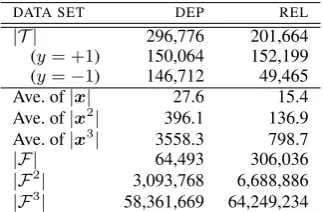
Table 1 summarizes the training data for the two tasks. The examples for the Japanese dependency parsing task were generated for a transition-based parser (Sassano, 2004) from a standard data set.6
We used the dependency accuracy of the parser
5The labeled data for dependency parsing is available
from: http://www.tkl.iis.u-tokyo.ac.jp/˜ynaga/pecco/, and the labeled data for hyponymy-relation extraction is avail-able from: http://nlpwww.nict.go.jp/hyponymy/.
6Kyoto Text Corpus Version 4.0:
http://nlp.kuee.kyoto-u.ac.jp/nl-resource/corpus-e.html.
DATA SET DEP REL
|T | 296,776 201,664
(y= +1) 150,064 152,199 (y=−1) 146,712 49,465 Ave. of|x| 27.6 15.4 Ave. of|x2| 396.1 136.9 Ave. of|x3| 3558.3 798.7
|F| 64,493 306,036
|F2
| 3,093,768 6,688,886
|F3
| 58,361,669 64,249,234
Table 1: Training data for dependency parsing (DEP) and hyponymy-relation extraction (REL).
as model accuracy in this task. In the hyponymy-relation extraction task, we randomly chosen two sets of 10,000 examples from the labeled data for development and testing, and used the remaining examples for training. Note that the number of active features,|Fd|, dramatically grows when we consider higher-order conjunctive features.
We compared the proposed method, PA-I SL (Algorithm 1 with Algorithm 2), to PA-I KER -NEL(Algorithm 1 with PKI; Okanohara and Tsu-jii (2007)),PA-I KE(Algorithm 1 with kernel ex-pansion; viz., kernel splitting with N = |F|),
SVM(batch training of support vector machines),7 and`1-LLM (stochastic gradient descent training
of the `1-regularized log-linear model: Tsuruoka
et al. (2009)). We refer to PA-I SL that does not reuse temporal partial margins as PA-I SL∗. To demonstrate the impact of conjunctive features on model accuracy, we also trainedPA-Iwithout con-junctive features. The number of iterations inPA-I was set to 20, and the parameters ofPA-Iwere av-eraged in an efficient manner (Daum´e III, 2006). We explicitly considered conjunctions among
top-N (N = 125×2n;n ≥ 0) features in PA-I SL andPA-I SL∗. The hyperparameters were tuned to maximize accuracy on the development set.
4.3 Results
Tables 2 and 3 list the experimental results for the two tasks (due to space limitations, Tables 2 and 3 listPA-I SLwith parameterN that achieved
the fastest speed). The accuracy of the models trained with the proposed method was better than
`1-LLMs and was comparable toSVMs. The
METHOD d ACC. TIME MEMORY
PA-I 1 88.56% 3s 55MB
`1-LLM 2 90.55% 340s 1656MB
SVM 2 90.76% 29863s 245MB
PA-I KERNEL 2 90.68% 8361s 84MB
PA-I KE 2 90.67% 41s 155MB
PA-I SL∗N=4000 2 90.71% 33s 95MB `1-LLM 3 90.76% 4057s 21,499MB
SVM 3 90.93% 25912s 243MB
PA-I KERNEL 3 90.90% 8704s 83MB
PA-I KE 3 90.90% 465s 993MB
PA-I SLN=250 3 90.89% 262s 175MB
Table 2: Training time for classifiers used in de-pendency parsing task.
0 300 600 900 1200 1500
102 103 104 105
T
ra
in
in
g
ti
m
e
[s
]
N: # of expanded primitive features
PA-I SP PA-I SL∗
PA-I SL
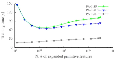
Figure 1: Training time forPA-Ivariants as a func-tion of the number of expanded primitive features in dependency parsing task (d= 3).
rior accuracy of PA-I (d = 1) confirmed the
ne-cessity of conjunctive features in these tasks. The minor difference among the model accuracy of the threePA-Ivariants was due to rounding errors.
PA-I SL was the fastest of the training meth-ods with the same feature set, and its space effi-ciency was comparable to the kernel-based learn-ers. PA-I SL could reduce the memory footprint from 993MB8to 175MB ford= 3in the
depen-dency parsing task, while speeding up training. Although linear training (`1-LLM andPA-I KE)
dramatically slowed down when we took higher-order conjunctive features into account, kernel slicing alleviated deterioration in speed. Espe-cially in the hyponymy-relation extraction task, PA-I SL took almost the same time regardless of the order of conjunctive features.
8`1-LLMtook much more memory thanPA-I KEmainly
because`1-LLMexpands conjunctive features in the
exam-ples prior to training, whilePA-I KEexpands conjunctive
fea-tures in each example on the fly during training. Interested readers may refer to (Chang et al., 2010) for this issue.
METHOD d ACC. TIME MEMORY
PA-I 1 91.75% 2s 28MB
`1-LLM 2 92.67% 136s 1683MB
SVM 2 92.85% 12306s 139MB
PA-I KERNEL 2 92.91% 1251s 54MB
PA-I KE 2 92.96% 27s 143MB
PA-I SL∗N=8000 2 92.88% 17s 77MB `1-LLM 3 92.86% 779s 14,089MB
SVM 3 93.09% 17354s 140MB
PA-I KERNEL 3 93.14% 1074s 49MB
PA-I KE 3 93.11% 103s 751MB
PA-I SLN=125 3 93.05% 17s 131MB
Table 3: Training time for classifiers used in hyponymy-relation extraction task.
0 30 60 90 120 150
102 103 104 105 106
T
ra
in
in
g
ti
m
e
[s
]
N: # of expanded primitive features
PA-I SP PA-I SL∗
PA-I SL
Figure 2: Training time forPA-Ivariants as a func-tion of the number of expanded primitive features in hyponymy-relation extraction task (d= 3).
Figures 1 and 2 plot the trade-off between the number of expanded primitive features and train-ing time with PA-I variants (d = 3) in the two
tasks. Here, PA-I SP is PA-I with kernel slicing without the techniques described in Sections 3.2.1 and 3.2.2, viz., kernel splitting. The early termi-nation of margin computation reduces the train-ing time whenN is large. The reuse of temporal
margins makes the training time stable regardless of parameter N. This suggests a simple,
effec-tive strategy for calibratingN; we start the
train-ing withN = |F|, and when the learner reaches the allowed memory size, we shrink N to N/2
by pruning sub-trees rooted by rarer features with RANK(f)> N/2in the weight trie.
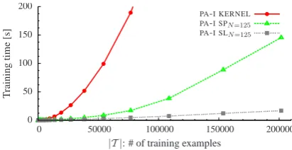
Figures 3 and 4 plot training time with PA-I variants (d = 3) for the two tasks as a function
0 100 200 300 400 500 600
0 50000 100000 150000 200000 250000 300000
T
ra
in
in
g
ti
m
e
[s
]
|T |: # of training examples
PA-I KERNEL PA-I SPN=250 PA-I SLN=250
Figure 3: Training time forPA-Ivariants as a func-tion of the number of training examples in depen-dency parsing task (d= 3).
5 Related Work
There are several methods that learn ‘simpler’ models with fewer variables (features or support vectors), to ensure scalability in training.
Researchers have employed feature selection to assure space-efficiency in linear training. Wu et al. (2007) used frequent-pattern mining to se-lect effective conjunctive features prior to train-ing. Okanohara and Tsujii (2009) revised graft-ing for`1-LLM(Perkins et al., 2003) to prune
use-less conjunctive features during training. Iwakura and Okamoto (2008) proposed a boosting-based method that repeats the learning of rules repre-sented by feature conjunctions. These methods, however, require us to tune the hyperparameter to trade model accuracy and the number of conjunc-tive features (memory footprint and training time); note that an accurate model may need many con-junctive features (in the hyponymy-relation ex-traction task,`1-LLMneeded 15,828,122 features
to obtain the best accuracy, 92.86%). Our method, on the other hand, takes all conjunctive features into consideration regardless of parameterN.
Dekel et al. (2008) and Cavallanti et al. (2007) improved the scalability of the (kernel) percep-tron, by exploiting redundancy in the training data to bound the size of the support set to given thresh-oldB (≥ |St|). However, Orabona et al. (2009) reported that the models trained with these meth-ods were just as accurate as a naive method that ceases training when|St|reaches the same thresh-old,B. They then proposed budget online
learn-ing based on PA-I, and it reduced the size of the support set to a tenth with a tolerable loss of
accu-0 50 100 150 200
0 50000 100000 150000 200000
T
ra
in
in
g
ti
m
e
[s
]
|T |: # of training examples
PA-I KERNEL PA-I SPN=125
PA-I SLN=125
Figure 4: Training time for PA-I variants as a function of the number of training examples in hyponymy-relation extraction task (d= 3).
racy. Their method, however, requiresO(|St−1|2)
time in updating the parameters in roundt, which
disables efficient training. We have proposed an orthogonal approach that exploits the data redun-dancy in evaluating the kernel to train the same model as the base learner.
6 Conclusion
In this paper, we proposed online learning with kernel slicing, aiming at resolving the space-time trade-off in training a classifier with many con-junctive features. The kernel slicing generalizes kernel splitting (Goldberg and Elhadad, 2008) in a purely feature-wise manner, to truly combine the merits of linear and kernel-based training. To im-prove the scalability of the training with redundant data inNLP, we reuse the temporal partial margins computed in past rounds and terminate unneces-sary margin computations. Experiments on de-pendency parsing and hyponymy-relation extrac-tion demonstrated that our method could train a classifier orders of magnitude faster than kernel-based learners, while retaining its space efficiency. We will evaluate our method with ample la-beled data obtained by the semi-supervised meth-ods. The implementation of the proposed algo-rithm for kernel-based online learners is available from http://www.tkl.iis.u-tokyo.ac.jp/˜ynaga/.
Acknowledgment We thank Susumu Yata for providing us practical lessons on the double-array trie, and thank Yoshimasa Tsuruoka for making his`1-LLM code available to us. We are also
References
Ando, Rie Kubota and Tong Zhang. 2005. A frame-work for learning predictive structures from multi-ple tasks and unlabeled data. Journal of Machine Learning Research, 6:1817–1853.
Aoe, Jun’ichi. 1989. An efficient digital search al-gorithm by using a double-array structure. IEEE Transactions on Software Engineering, 15(9):1066– 1077.
Bellare, Kedar, Partha Pratim Talukdar, Giridhar Ku-maran, Fernando Pereira, Mark Liberman, Andrew McCallum, and Mark Dredze. 2007. Lightly-supervised attribute extraction. InProc. NIPS 2007 Workshop on Machine Learning for Web Search. Cavallanti, Giovanni, Nicol`o Cesa-Bianchi, and
Clau-dio Gentile. 2007. Tracking the best hyperplane with a simple budget perceptron. Machine Learn-ing, 69(2-3):143–167.
Chang, Yin-Wen, Cho-Jui Hsieh, Kai-Wei Chang, Michael Ringgaard, and Chih-Jen Lin. 2010. Train-ing and testTrain-ing low-degree polynomial data map-pings via linear SVM. Journal of Machine Learning Research, 11:1471–1490.
Crammer, Koby, Ofer Dekel, Joseph Keshet, Shai Shalev-Shwartz, and Yoram Singer. 2006. Online passive-aggressive algorithms. Journal of Machine Learning Research, 7:551–585.
Daum´e III, Hal. 2006. Practical Structured Learn-ing Techniques for Natural Language ProcessLearn-ing. Ph.D. thesis, University of Southern California. Daum´e III, Hal. 2008. Cross-task
knowledge-constrained self training. In Proc. EMNLP 2008, pages 680–688.
Dekel, Ofer, Shai Shalev-Shwartz, and Yoram Singer. 2008. The forgetron: A kernel-based percep-tron on a budget. SIAM Journal on Computing, 37(5):1342–1372.
Freund, Yoav and Robert E. Schapire. 1999. Large margin classification using the perceptron algo-rithm. Machine Learning, 37(3):277–296.
Goldberg, Yoav and Michael Elhadad. 2008. splitSVM: fast, space-efficient, non-heuristic, poly-nomial kernel computation for NLP applications. In
Proc. ACL-08: HLT, Short Papers, pages 237–240. Isozaki, Hideki and Hideto Kazawa. 2002. Efficient
support vector classifiers for named entity recogni-tion. InProc. COLING 2002, pages 1–7.
Iwakura, Tomoya and Seishi Okamoto. 2008. A fast boosting-based learner for feature-rich tagging and chunking. InProc. CoNLL 2008, pages 17–24.
Kudo, Taku and Yuji Matsumoto. 2003. Fast methods for kernel-based text analysis. InProc. ACL 2003, pages 24–31.
Liang, Percy, Hal Daum´e III, and Dan Klein. 2008. Structure compilation: trading structure for fea-tures. InProc. ICML 2008, pages 592–599. Okanohara, Daisuke and Jun’ichi Tsujii. 2007. A
dis-criminative language model with pseudo-negative samples. InProc. ACL 2007, pages 73–80.
Okanohara, Daisuke and Jun’ichi Tsujii. 2009. Learn-ing combination features withL1regularization. In
Proc. NAACL HLT 2009, Short Papers, pages 97– 100.
Orabona, Francesco, Joseph Keshet, and Barbara Ca-puto. 2009. Bounded kernel-based online learning.
Journal of Machine Learning Research, 10:2643– 2666.
Perkins, Simon, Kevin Lacker, and James Theiler. 2003. Grafting: fast, incremental feature selection by gradient descent in function space. Journal of Machine Learning Research, 3:1333–1356. Sassano, Manabu. 2004. Linear-time dependency
analysis for Japanese. In Proc. COLING 2004, pages 8–14.
Sumida, Asuka, Naoki Yoshinaga, and Kentaro Tori-sawa. 2008. Boosting precision and recall of hy-ponymy relation acquisition from hierarchical lay-outs in Wikipedia. In Proc. LREC 2008, pages 2462–2469.
Tsuruoka, Yoshimasa, Jun’ichi Tsujii, and Sophia Ananiadou. 2009. Stochastic gradient descent training for L1-regularized log-linear models with cumulative penalty. In Proc. ACL-IJCNLP 2009, pages 477–485.
Williams, Hugh E. and Justin Zobel. 1999. Compress-ing integers for fast file access.The Computer Jour-nal, 42(3):193–201.
Wu, Yu-Chieh, Jie-Chi Yang, and Yue-Shi Lee. 2007. An approximate approach for training polynomial kernel SVMs in linear time. InProc. ACL 2007, In-teractive Poster and Demonstration Sessions, pages 65–68.
Yata, Susumu, Masahiro Tamura, Kazuhiro Morita, Masao Fuketa, and Jun’ichi Aoe. 2009. Sequential insertions and performance evaluations for double-arrays. In Proc. the 71st National Convention of IPSJ, pages 1263–1264. (In Japanese).