Emerging Quantum Fields Embedded in the
Emergence of Spacetime
Hans Diel
1 2 3
4 5 6 7
8 9 10 11
12 13 14
15
DielSoftwareBeratungundEntwicklung,Seestr.102,71067Sindelfingen,Germany,[email protected]
Abstract: Basedon alocalcausalmodelof thedynamicsof curveddiscrete spacetime,acausal modelofquantumfieldtheoryincurveddiscretespacetimeisdescribed.Attheelementarylevel, space(-time)isassumedtoconsistsofinterconnectedspacepoints. Eachspacepointisconnected toasmalldiscretesetofneighborspacepoints. Densitydistributionofthespacepointsandthe lengthsofthespacepointconnectionsdependonthedistancefromthegravitationalsources.This leadstocurvedspacetimeinaccordancewithgeneralrelativity. Dynamicsofspacetime(i.e.,the emergenceofspaceandthepropagationofspacechanges)dynamicallyassigns"in-connections" and "out-connections" to the affected space points. Emergence and propagation of quantum fields( includingp articles)a rem appedt ot hee mergencea ndp ropagationo fs pacec hangesby utilizingidenticalpathsofin/out-connections.Compatibilitywithstandardquantumfieldtheory (QFT)requeststhe adjustmentof theQFTtechniques(e.g., Feynman diagrams,Feynman rules, creation/annihilationoperators),whichtypicallyapplytothreein/outconnections,ton>3in/out connections.Inaddition,QFTcomputationinpositionspacehastobeadaptedtoacurveddiscrete space-time.
Keywords:quantumfieldtheory,localcausalmodels,generalrelativitytheory,spacetimemodels, discretespacetime,computersimulations
16
1. Introduction
17
The authors attempt to construct a local causal model of quantum theory (QT), including quantum 18
field theory (QFT), soon resulted in the recognition that a causal model of the dynamics of QT/QFT 19
should better be based on a causal model of the dynamics of spacetime. Thus, a causal model of the 20
dynamics of spacetime has been developed with the major goals (1) as much as possible compatibility 21
with general relativity theory (GRT), and (2) the model should match the main features of the evolving 22
model of QT/QFT. The main features of the authors model of QT/QFT are 23
• the model has to be a causal model, 24
• if possible, the model should be alocalcausal model, 25
• discreteness of the basic parameters (time, space, propagation paths). 26
Not surprisingly, it turned out that a clear definition of these features/requirements, especially of a 27
local causal model, is useful (not only for understanding the requirements, but also for the derivation 28
of the implications). A semi-formal definition of a (local) causal model has been published in several 29
articles from the author (see [1], [2] and [3]) and is also given in Section 2. 30
The construction of a causal model of spacetime dynamics started with the search for some 31
existing theory or model which might be at least a starting point for the model to be developed. Causal 32
dynamical triangulation (CDT, see [4], [5], [6]) and more abstractly the concepts of loop quantum 33
gravity (see [7] and [8]) were identified to match the authors requirements and thinking. The further 34
model construction showed that, in order to come up with a local causal model according to the 35
definitions given in Section 2, adaptations and refinements of the original CDT-based model appear 36
appropriate. The adaptations and refinements concern basic GRT concepts such as (i) the elementary 37
structure of space(-time), (ii) the representation of space(-time) curvature, and (iii) the relation between 38
space and time. With GRT and special relativity theory (SRT), space and time are said to be integrated 39
into spacetime. For the GRT-compatible model of spacetime dynamics, the integration of space and 40
time remains, but with a different interpretation. The elementary structure of space(-time), including 41
the space-time relationship is described in Section 3. The causal model of the spacetime dynamics is 42
described in Section 4. 43
The major goal for the development of a causal model of spacetime dynamics (Sections 3 and 44
4) was to develop a model of the spacetime elementary structure that constitutes a suitable base 45
for both the causal model of spacetime dynamics and the causal model of QT/QFT. The proposed 46
model satisfies this goal. The emergence and propagation of quantum fields (including particles) 47
can be mapped to the emergence and propagation of space changes by utilizing identical paths of 48
in/out-connections between space points. In Section 5, this main subject of the article is described. 49
2. Causal Models
50
The specification of a causal model of a theory of physics consists of (1) the specification of the 51
system state, (2) the specification of the laws of physics that define the possible state transitions when 52
applied to the system state, and (3) the assumption of a “physics engine.” 53
2.0.1. The physics engine 54
The physics engine represents the overall causal semantics of causal models. It acts upon the state 55
of the physical system. The physics engine continuously determines new states in uniform time steps. 56
For the formal definition of a causal model of a physical theory, a continuous repeated invocation of 57
the physics engine is assumed to realize the progression of the state of the system. 58
59
physics engine(S,∆t):={ 60
DO UNT IL(nonContinueState(S)){ 61
S←applyLawsO f Physics(S,∆t); 62
} 63
} 64
2.0.2. The system state 65
The system state defines the components, objects and parameters of the theory of physics that can 66
be referenced and manipulated by the causal model. In contrast to the physics engine, the structure 67
and content of the system state are specific for the causal model that is being specified. Therefore, the 68
following is only an example of a possible system state specification. 69
70
systemstate:={spacepoint...} 71
spacepoint:={x1,x2,x3,ψ}
72
ψ:={stateParameter1, ...,stateParametern} 73
74
2.0.3. The laws of physics 75
The refinement of the statement 76
S←applyLawsO f Physics(S,∆t); defines how an "in" state s evolves into an "out" state s. 77
L1:= IF c1(s)THEN s← f1(s); 78
L2:= IF c2(s)THEN s← f2(s); 79
... 80
Ln := IF cn(s)THEN s← fn(s); 81
The "in" conditionsci(s)specify the applicability of the state transition function fi(s)in basic formal 82
(e.g., mathematical ) terms or refer to complex conditions that then have to be refined within the formal 83
The state transition functionfi(s)specifies the update of state s in basic formal (e.g., mathematical) 85
terms or refers to complex functions that then have to be refined within the formal definition. 86
The set of lawsL1, ...,Lnhas to be complete, consistent and reality conformal (see [9] for more details). 87
In addition to the above-described basic forms of specification of the laws of physics byLn :=
88
IF cn(s)THEN s← fn(s), other forms are also imaginable and sometimes used in this article.1 89
2.1. Requirements for causal models of spacetime 90
For causal models of spacetime, obviously, some notion of space and time must be supported. 91
Ideally, the treatment of space and time would be, as much as possible, compatible with special 92
relativity theory (SRT) and general relativity theory. However, the formally defined causal model 93
of Section 2 presupposes a certain structure of spacetime in which space and time are rigorously 94
separated. This disturbs the integrated view of space and time that is taught by GRT/SRT. In the 95
proposed model of spacetime dynamics, the integration of space and time is largely restored by the 96
specification of the relationships described in Section 3.1. 97
2.1.1. The representation of time in the causal model 98
In the causal model defined above, time is not like space and other parameters a system state 99
component, but it has a special role outside the system state. The overall purpose of the causal model 100
is seen in showing the progression of the system state in relation to the progression of time. This 101
relationship can best be described by assuming a uniform progression of the time. This leads to the 102
model (described above) where the time and the progression of time is built into the model in the form 103
of the physics engine. The physics engine progresses the system state in uniform time steps called 104
state update time intervals (SUTI). 105
In GRT and SRT, there are situations where the clock rate of a causal subsystem is predicted to 106
differ depending on the relative speed of movement or the position within a gravitational field. GRT 107
and SRT refer to this by the name "proper time". If, for a specific causal model of an area of physics 108
the differing proper times of causal subsystems are relevant and/or the internal processes within the 109
subsystems are included in the model, separate physics engines may be assigned to the subsystems 110
with different proper times.2 111
If, however, the causal model describes an area of physics where the relationship between proper 112
times and other parameters is to be shown, it should be possible to show this with a single physics 113
engine and a uniform SUTI for the overall system. For the proposed causal model of spacetime 114
dynamics, the space-time relationship described in Section 3.1 enables a single physics engine and a 115
uniform SUTI. 116
2.1.2. Spatial causal model 117
A causal model of a theory of physics is called aspatialcausal model if (1) the system state contains 118
a component that represents a space, and (2) all other components of the system state can be mapped 119
to the space. There exist many textbooks on physics (mostly in the context of relativity theory) and 120
mathematics that define the essential features of a "space". For the purpose of the present article, a 121
more detailed discussion is not required. For the purpose of this article and the subject locality, it is 122
sufficient to request that the space (assumed with a spatial model) supports the notions of position, 123
coordinates, distance, and neighborhood. 124
1 This article does not contain a proper definition of the used causal model specification language. The language used is
assumed to be largely self-explanatory.
2 An example can be found in the causal model described in [3], where separate physics engines are assigned to the "quantum
A special type of spatial causal model that has been increasingly addressed in recent years is 125
the cellular automaton (see [10], [11], [12] and [13]). The causal model described in this article also 126
represents a spatial causal model. 127
2.1.3. Local causal model 128
The definition of a local causal model presupposes a spatially causal model (see above). A 129
(spatially) causal model is understood to be a local model if changes in the state of the system 130
depend on the local state only and affect the local state only. The local state changes can propagate to 131
neighboring locations. The propagation of the state changes to distant locations; however, they must 132
always be accomplished through a series of state changes to neighboring locations.3 133
Based on a formal model definition of a causal model, a formal definition of locality can be 134
given. A physical theory and a related spatially causal model with position coordinates x and position 135
neighborhood dx (or∆xin the case of discrete space-points) are given. A causal model is called a 136
local causal model if each of the lawsLi applies to no more than a single position x and/or to the 137
neighborhood of this positionx±dx. 138
In the simplest case, this arrangement means thatLihas the form 139
Li: IF ci(s(x))THENs0(x) = fi(s(x)); 140
The position reference can be explicit (for example, with the above simple case example) or implicit by 141
reference to a state component that has a well-defined position in space. References to the complete 142
space of a spatially extended object or to a property of a spatially extended object are considered 143
to violate "space-point-locality". Causal models with a system state that includes composite objects 144
with global properties (e.g., mass, charge, velocity) may still be considered local causal models, more 145
specifically "object-local causal model", even if such global properties are referenced in the model. 146
2.1.4. Background-independence 147
Background independence is an important requirement that is typically established for spacetime 148
models such as spin networks, spin foam, and causal dynamical triangulation. This requirement seems 149
to be mandatory for a local causal spacetime model that supports the emergence of spacetime from a 150
minimal or zero source. Background independence means that all spacetime dynamics, in particular 151
the emergence of space, must be expressible without reference to any predefined coordinate system or 152
other global spacetime properties. For a causal model, this means that the structure of spacetime must 153
not contain components and properties that are non-local. 154
2.1.5. Composite objects 155
Models of areas of physics typically contain spatially extended composite objects such as particles, 156
atoms, stars, and so forth, and typically object-global properties (e.g., mass, charge, velocity) are 157
referenced in such models. According to the definition of a local causal model (above), such models 158
may only be called "object-local causal models" (as opposed to "space-point-local causal models"). Such 159
models may be useful; however, care must be taken that the assignment of object-global properties 160
to composite objects is admissible with the level of accuracy aimed for. Object-global properties are 161
typically the result of aggregations from lower-level relationships. The aggregations toward a single 162
global attribute value may be admissible with classical physics, but questionable with refinements of 163
modern theories of physics. A famous example of the inclusion of global object properties refers to the 164
attributes of mass and charge with quantum field theory when particles are no longer considered to be 165
point-like particles. 166
3 Special relativity requests that the series of state changes does not occur with a speed that is faster than the speed of light.
3. The elementary structure of spacetime
167
3.1. The space-time relationship 168
With GRT and SRT, space and time are said to be integrated into spacetime. For a GRT-compatible 169
model of spacetime dynamics, the integration of space and time remains visible, but with a different 170
interpretation. With GRT, the integration of space and time is mathematically expressed in the usage of 171
tensors (e.g., curvature tensor) and 4-vectors with a time component and space components. Physically, 172
the integration is reflected, among other ways, in the metric and the symmetries that hold for the 173
combined (space+time) entities and the corresponding laws of physics. 174
In the proposed causal model of spacetime dynamics, the tensors and 4-vectors of GRT/SRT 175
occur only as the starting point for the introduction of GRT-compatible equivalent model parameters. 176
The integration of space and time appears to be disturbed by the fundamentally different roles space 177
and time represent in a causal model. Time and the progression of time are an inherent feature of the 178
physics engine of the causal model. The physics engine implements the uniform and simultaneous 179
progression of time. Space is the explicit global object that is part of the system state. Other objects of 180
the system state are positioned in space. Although space and time conceptually have quite different 181
roles within the causal model, it is their mutual relationship that establishes their (re-)integration. 182
In GRT, the curvature specification, i.e., the curvature tensor, contains, in addition to the three space-related components, a time-related component. As an example of the impact of the time factor, the gravitational redshift is explained as the consequence of the time factor in the spacetime curvature (see, for example, [14], page 231).
∆s2=−(1−2GM c2r )(c∆t)
2+ (∆x)2+ (∆y)2+ (∆z)2 (1)
This means a clock at position (x, y, z) would run by a factor
F1=
r
1−2GM
c2r (2)
slower than a clock that is not affected by a gravitational field. A standard clock at some point A of 183
low potential (for example, on the surface of the earth) would go slower than the same clock at point B 184
of higher potential (for example, at a GPS satellite). In [14]: "... The gravitational redshift implies that 185
time itself runs slightly faster at the higher altitude than it does on the Earth." For the GPS system, the 186
difference is 45 microseconds per day: This is the rate at which the clocks at the satellites go faster (see 187
[15]). In GRT, this effect is called "gravitational time dilation". For reasons that are described in the 188
following, the author prefers the wording (gravitational) "clock rate dilation". 189
For a mapping of the time factor of the GRT curvature specification to the proposed spacetime 190
model, two problems arise: 191
1. In the causal model, the clock rate (i.e., the proper time) is a property of the whole causal 192
subsystem. The assignment of clock rates to the different positions occupied by a spatial 193
distributed causal subsystem is not supported with the proposed causal model.4 194
2. In the causal model, the clock rate is maintained by the physics engine (i.e., the clock is part of 195
the physics engine which delivers the uniform state update time interval). Changes in the clock 196
rate resulting from the objects motion in space would mean that the clock of the physics engine 197
has to run slower or faster depending on the object’s position in space. This would require a 198
rather ugly interface between the space and the physics engines of the causal subsystems. 199
4 The assignment of differing clock rates to the different positions occupied by a spatial distributed causal subsystem would
Problem (2) may be viewed as a problem due to the specific definition of a causal model given in 200
Section 2. However, there are (good) reasons for this definition of a causal model. Problem (1) refers to 201
the causal model of causal subsystems in general. It would also be difficult to avoid this problem with 202
alternative causal model concepts. 203
A possible solution that would make it possible to maintain a uniform progression of the state 204
update time interval SUTI while enabling non-uniform clock rates may be found if one remembers 205
that, in SRT and GRT, space and time are considered as an entity and that this implies that space 206
intervals and time intervals can be jointly transformed by certain symmetry transformations. For 207
the example gravitational redshift, this means that the redshift is interpreted as the dilation of the 208
wave length instead of the increase of the frequency and that the length dilation affects not only the 209
wave length but all lengths within the gravitational potential. For the proposed model of spacetime 210
dynamics, it is assumed that 211
212
Proposition 1. Lengths within the gravitational field are dilated by the factor F1. 213
5How can this help to prevent the need for the dynamic and position-dependent change of the 214
state update time interval (SUTI)? A further proposition was introduced: 215
Proposition 2. Physical processes run faster/slower depending on the length scale at the position where the 216
respective physical process executes. 217
Notice that the clock rate dilation concerns physical processes, not the spacetime structure. 218
Space(-time) curvature is the result of length dilations. Clock rate dilation is another consequence of 219
length dilations. 220
The major process that demonstrates the fixed relationship between the length dilation and the 221
process change rate is the propagation of light. This (simple) process is used as a measure for the 222
change rate of other processes by setting the speed of light to be a constant c. The next class of 223
processes where the change rate depends on the length dilation in precisely the proportions as with 224
the propagation of light are clocks in differing realizations. 225
In summary, in the model of spacetime dynamics, there is no direct reflection of time dilation as a 226
spacetime attribute. Clock rate dilation (rather than time dilation) occurs as a property of processes 227
running within space. The clock rate dilation factor can be derived from the length dilation factorF1of 228
the space points where the respective process is currently executing. 229
In the model of spacetime dynamics, two levels of time are distinguished, which in GRT/SRT are 230
seen as an entity: 231
1. At the basic level, the progression of time is associated with the physics engine of the causal model. 232
The time of the physics engine proceeds in uniform state update time intervals. Simultaneousness 233
is assumed for all state changes occurring at the same state update cycle. 234
2. Differing clock rates, proper times, and relativity of simultaneousness are not associated with the 235
basic overall spacetime, level (1), but are associated with objects residing and moving in space -236
more precisely, with processes running in these subsystems. 237
With space, two levels also may be distinguished, but these are two levels of consideration: 238
5 "Gravitational length dilation" appears to be a very controversial subject among physicists (see various discussion in internet
• At the abstract level (i.e., mathematical level), the space consists of a set of interconnected space 239
points (see Section 3). Whether or not the totality of interconnected space points represents an 240
Euclidean space or a specific topology (e.g., Riemann manifold) is left open. 241
• At the physical level (i.e., the essential level), meaning is assigned to the components of the space 242
point. Especially, the length of the connections is no longer a geometrical property, but specifies 243
the∆lengthonlywith respect to a specific physical process executing at the respective space point 244
for the time interval SUTI. The process that is used as the measure for the specification of the 245
length is the propagation of light. 246
Thus, the integration of space and time into spacetime is established in the model of spacetime 247
dynamics by the physical meaning assigned to the components of the space points and their 248
connections. 249
1. Time progresses uniformly in constant units. As a suitable basic unit of time progression, the 250
state update time interval (SUTI) of the physics engine is taken. This means, the SUTI is assumed 251
to be a system constant. 252
2. Length specification is expressed in relation to the spatial distance change caused by a specific 253
physical process running for the duration of the standard unit of time (i.e., the SUTI).6 254
3. The physical process that is used as the measure for the standard unit of time as well as the 255
measure of spatial distances is the propagation of light.7 256
The proposition (fact?) that there is such a simple relationship between the spatial length dilations 257
and the rate of state changes of processes that execute at a given position in space is the root of the 258
space-time integration in the proposed model of spacetime dynamics. A possible foundation of this 259
supposed space-time relationship (reflecting the space-time integration) may be that 260
Conjecture 3.1. All physical processes can ultimately be broken down to length-related state changes, 261
and changes in the length scaling therefore directly result in clock rate dilations of the affected process. 262
3.2. The elementary structure of space 263
The proposed elementary structure of spacetime constitutes the base for the overall model of 264
spacetime dynamics that is compatible with GRT. A number of works toward the same or a similar 265
goal have been published. The work that shows the most similarities with the model described in this 266
article in terms of the overall orientation (background independence; discreteness of time, space, and 267
paths; expressing causal relationships) is causal dynamical triangulation (CDT, see [4], [5], and [6]). 268
The spacetime structure of the model described in this article is based on CDT. However, it was felt 269
that adaptations were required to further refine the causal relationships of spacetime dynamics, in 270
particular to construct a causal model of the emergence of space from a single source. 271
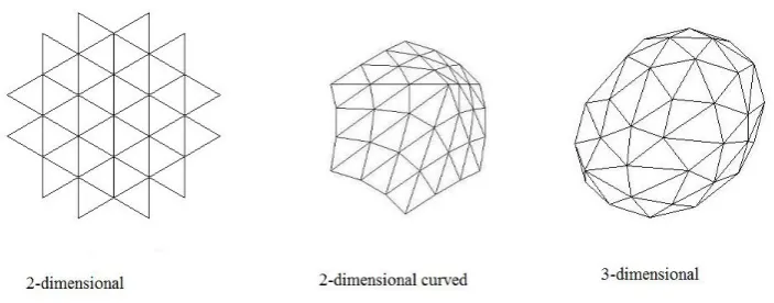
With CDT, the basic space elements are n-dimensional simplexes (e.g., triangles, tetrahedrons; see 272
Fig.1). In contrast to CDT, the proposed causal model of curved discrete spacetime considers only 273
3-dimensional space elements, i.e., tetrahedrons. The time dimension is treated separately within the 274
causal model. In addition, the elementary units that represent the total space are not (as with CDT) 275
the n-dimensional simplexes, but only the space points together with their connections to neighbor 276
space points8. Whether the space points together with the connections establish specific 2-dimensional 277
surface areas (e.g., triangles) and 3-dimensional solids (e.g., tetrahedrons) is initially left open. 278
6 This means, in the causal model, spatial distances are not primarily a geometrical property, but rather a physical property
used to formulate interrelationships between objects in space.
7 This has the consequence, that in the model (as with most models of physics), the speed of light c is a constant.
8 The reason for this simplification was that it was not possible to build up a larger space object by the continuous addition of
Figure 1.Elements of spacetime of Causal Dynamical Triangulation.
Definition 1. Space := { spacepoint ...}; 279
spacepoint := {ψ,dilation f actor,connections };
280
connections := { connection1, ...,connectionn}; 281
connection := { neighborspacepoint,direction,∆curvature }; 282
ψis the physical content that is directly associated with the space. These are the fields residing
283
in space. As with spin networks, spin foam networks, and causal dynamical triangulation, each 284
space point is connected with a number of other space points via "connections" (i.e., edges in CDT). A 285
connection carries the information about the connected neighbor space point, the connection direction, 286
and the propagation gradient of the curvature changes (see Section 4). 287
All the information associated with the space point is local to the space point (i.e., no globally 288
defined position or direction specification). This supports the background independence of the 289
spacetime model. 290
To enable the determination of the spatial distance between two space points, some information 291
about the distance between neighbor space points is required. This could be provided, for example, 292
in form of position coordinates9or by the specification of the lengths of connections between the 293
neighbor space points. In support of a causal model of the movement of objects in curved space, for 294
the proposed model of spacetime dynamics, it is defined that 295
Proposition 3. The length of the connections between space points is a constant; 296
Lconnection =c·SUT I. 297
The overall distance between two space points within the curved space is then obtained by 298
multiplyingLconnection by the number of space pointskpon the geodesic path from space point-1 to 299
space point-2. Length dilation within a gravitational potential as assumed by Proposition 1 in Section 300
3.1, is realized by the appropriate arrangement of the space points within space (see Section 4). 301
Proposition 3 is, first of all, a physical statement, although it has consequences for the space 302
geometry. The physical statement is: 303
The (spatial) distance that light moves during a state update time interval (SUTI) is equal to the distance 304
between two connected neighbor space points, which is equal to the distance by which space expands during a 305
SUTI. 306
The geometry of the emerged space (e.g., whether an Euclidean space or a Schwarzschild metric 307
emerges) depends on the space expansion algorithm. With the proposed model of spacetime dynamics 308
the resulting geometry depends on the ratio by which the number of space points grow at a single 309
expansion step (see Section 4.1). 310
3.3. The representation of space(-time) curvature 311
Space curvature is a major ingredient of GRT. In GRT, specifically in Einstein’s equation 312
Gαβ=8πTαβ,
313
space curvature is expressed by the curvature tensorGαβ. Thus, the simplest solution would be to say
314
that a space-curvature component is assigned to the space point and that this curvature specification 315
provides the same information as the curvature tensor of GRT. However, some adaptations appear 316
reasonable. In Section 3.2 above, the space component of the system state is specified as consisting 317
of a set of space points, and, at the next level of detail, a space point is specified as consisting of 318
dilationfactor, connections, and the space contentψ.
319
spacepoint := {ψ,dilation f actor,connections};
320
The dilationfactor supports the generation of the space curvature with the propagation of space 321
changes (including the emergence of space). Once the space has emerged, the space(-time) curvature 322
is represented by (1) the distribution and density of the space points and (2) the (spatial) distances 323
between neighboring space points. Proposition 3 (above) states that the length of the connections 324
between space points, i.e., the distances between neighboring space points, is a constant. Thus, the 325
main parameter that determines the space curvature is the density distribution of the space points. 326
The density distribution of space points is realized by the appropriate arrangement of the space points 327
within space. 328
As described in Section 3.1, Proposition 2, the the clock rate dilation (i.e., the time-related 329
component of the GRT curvature) is a consequence of the length dilations. This means that the 330
information which specifies the length dilations implies the time-related component of the GRT 331
curvature. 332
4. Space(-time) dynamics
333
The dynamics of spacetime is triggered by the minimal sources, called "quantum objects". With 334
each update cycle of the system state a new space change action starts at each quantum object. The 335
space changes propagate from the quantum objects through the whole space in steps according to the 336
update cycles of the physics engine. In support of alocalcausal model, with each update cycle, the 337
space changes propagate only to (part of) the neighboring space points. The propagating space changes 338
always have definite directions at each space point, from the "in-connections" to the "out-connections" 339
of the space point. The out-connections of space point sp, at a given update cycle i, are in-connections 340
of some neighbor space points of sp with the subsequent update cycle i+1. 341
The directions of space changes, i.e., the identification of in/out-connections, are determined 342
by the∆curvatureattribute of the space point connections. For a given space point, only part of 343
the connections can be in-connections, which meansconnection.∆curvature > 0. The remaining 344
connections of the space point are out-connections. 345
The overall process of space change propagation is specified as 346
Specification 1. spaceprogression():={ 347
FOR ( all space pointsspi){ 348
IF ( inconnections(spi) { 349
propagateOUT(spi); 350
} } 351
4.1. The emergence of space from a single source 353
The space that emerges from a single source represents a Schwarzschild metric. In the causal 354
model, the large-scale space object emerges by the successive addition of surface layers to the initial 355
space object. 356
357
SSspaceemergence( source ) ::= { 358
spaceobject←source; 359
DO UNT IL(nonContinueState(S)){ 360
spaceobject←extendbynextlayer(spaceobject); 361
} 362
} 363
For the refinement of the above space emergence process, answers to the following questions have to 364
be provided: 365
1. What are the elementary units of space? 366
2. How does the initial space object look like? 367
3. What is the detailed algorithm forextendbynextlayer(spaceobject)? 368
4.1.1. The elementary units of space 369
The elementary structure of space, including the elementary units of space, have already been 370
described in Section 3.2. In the proposed model, the elementary units of space are the space points 371
together with their connections to neighbor space points (see Definition 1). The number of connections 372
(and thus the number of neighbor space points) of a given space point must be large enough to span 373
the complete three-dimensional space. It should be small enough to enable a moderate growth of the 374
number of space points with the chosen algorithm of the space emergence process. In the model, a 375
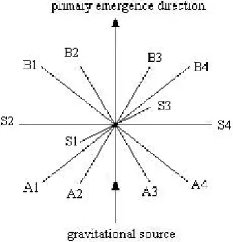
typical space point has 14 connections (see Fig.2): 376
• source connection: one connection towards the source of the emerging space, 377
• target connection: one connection in the primary emerging direction, 378
• surface connections: four connections in the plane that is perpendicular to the source connection 379
(S1, S2, S3, S4 in Fig.2), 380
• four connections in between the source connection and the surface connections (A1, A2, A3, A4 381
in Fig.2), 382
• four connections in between the target connection and the surface connections (B1, B2, B3, B4 in 383
Fig.2). 384
4.1.2. The initial space object 385
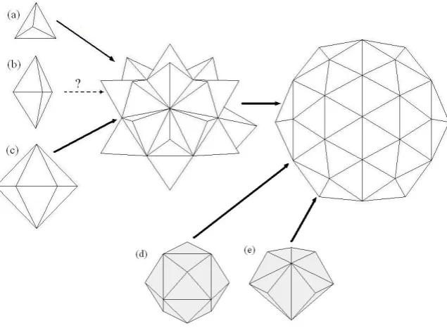
There are several alternatives for the initial space object from where the emergence of space and 386
the propagation of gravitational space dynamics may start. Fig. 3shows a number of alternatives 387
investigated by the author. The simplest solution would be to have the space emergence process, 388
starting from a single tetrahedron (case (a) in Fig. 3) or a double-tetrahedron (case (b) in Fig. 3) . 389
However, more symmetrical initial space objects, such as case (c) or case (d) enable the early emergence 390
of a symmetrical larger space object through simple space extension algorithms. For the present model 391
of spacetime dynamics the initial space object is a single space point surrounded by 14 neighbor space 392
points and the respective connections. The 14 neighbor space points, together with the interconnections 393
among them represent a spherical surface - the initial surface from where the space emergence starts 394
(case (d) in Fig.3). 395
4.1.3. The space expansion algorithm-extendbynextlayer(spaceobject)
396
As described above, space emergence from a single source is a continuous process where each 397
Figure 2.The 14 standard connections of a space point.
Table 1.Layers of space expansion, constant surface∆r=1.0
Layer surface surface total radius, av. edge
number triangles, kt points, kp . points, kpt ri length, L
0 12 8 8 1.00 1.63
1 36 20 72 2.00 1.72
2 108 56 228 3.00 1.55
3 324 164 660 4.00 1.22
4 972 488 1956 5.00 .88
... ... ... ... ... . ...
12 6377292 3188648 12754596 13.00 ...
13 19131876 9565940 38263764 14.00 ...
14 57395628 28697816 114791268 15.00 ...
... ... ... ... ... ...
i 3·kti−1 kpi−1+kti−1 ksi+3kpi−1 (i+1)100
This means, with each expansion stepstia numberkpiof new space points is generated. The new space 399
points are interconnected with their respective neighbor space point, formingktisurface triangles. 400
Various kinds of space expansion algorithms are possible. The key differentiating parameters for 401
the alternative space expansion algorithms are the growth factor gp of the number of surface space 402
points (i.e.,kpi=gp·kpi−1) and the related growth factor gt of the number of surface triangles (i.e., 403
kti =gt·kti−1). Table 1 shows the major parameters for an example space emergence algorithm that 404
starts with an initial space object with 12 surface triangles (case (c) in Fig. 3). The surface growth 405
factorgt=3, i.e.,kti =3·kti−1. The number of surface space points increases by the number of surface 406
triangles,kpi=kpi−1+kti−1. 407
Further parameters shown in Table 1 are the total number of space points, the radiusriof the surface 408
and the average edge length, L of the surface triangles. The average edge length, L is the length 409
measured by the author’s computer simulations and these computer simulations and the length 410
measurements assumeEuclidean space. However,the space emergence process of the model of spacetime 411
dynamics has to generate curved spacethat adheres to Schwarzschild metric, with length dilations in 412
accordance with the Propositions 1, 2 and 3. Especially, Proposition 3 says thatLconnectionis constant. 413
With the example shown in Table 1,Lconnection = ∆r = 1.0. This means that the circumference of a 414
surface, if curved space andLconnection = 1.0 is assumed, depends solely on the number of surface 415
space points,kpi. The number of surface space points,kpifor a surfaceSiis determined by the space 416
Figure 3.Alternative initial space elements.
dilations according toF1at the surfaces (see Eq. 2) has to emerge. This can only be achieved with 418
a decreasing growth factor gp. The space expansion algorithms that have been investigated by the 419
author showed that with the proposed model, GRT compatible space expansion algorithms are feasible. 420
However, unless the algorithm gets unnaturally complex, occasional inhomogeneities seem to be 421
unavoidable. In particular at the very small scale, i.e., near the minimal gravitational sources, it 422
appears to be difficult or impossible to preserve the GRT compatible behaviour.10 423
4.2. The propagation of space changes caused by multiple sources 424
The assumption that space changes start at the minimal sources implies that the aggregation of 425
space changes from many sources is the normal case. The model of the propagation of space changes 426
that are caused by multiple sources is based on the single-source propagation (Section 4.1). The 427
aggregation of the single-source propagations has to be accomplished by a local causal process, i.e., 428
by a series of aggregations of neighboring space changes. Only long range, this dynamical process, 429
can achieve overall gravitational space changes (i.e., curvature changes) that are compatible with the 430
predictions of GRT and Newtonian dynamics. 431
To simplify the description, in this article, "multiple sources" is initially equated to "two sources". 432
In simple cases, the treatment of many sources can be performed by a series of two source propagation 433
processes. 434
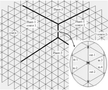
For the overall two-source propagation process, three phases can be distinguished: 435
• Phase-1, the phase where the changes from the two sources propagate independently. 436
• Phase-2, the phase where the changes start to overlap and therefore have to be aggregated. 437
• Phase-3, the phase where the aggregated changes propagate like single source changes. 438
10 The surrender of perfect GRT compatibility at the very small scale may ease the provision of a causal model of the dynamics
Figure 4.Propagation of space changes caused by 2 sources.
Fig.4shows an example snapshot in two dimensions, with the areas that are covered by phase-1 and 439
phase-3 roughly indicated.11 440
A major assumption of the proposed model is that the propagation that occurs at a space point 441
sp has a definite (consolidated) in-direction and the same (overall) out-direction. The consolidated 442
in-direction is the vector sum of the multiple in-connections. The overall out-direction is distributed 443
over the multiple out-connections. 444
4.2.1. Phase-1: 445
The propagation of space changes prior to the points where the changes meet is exactly the single 446
source propagation described in Section 4.1. 447
4.2.2. Phase-2: 448
When the space changes originating from (two) different sources meet at space point sp, the 449
changes that arrive from n space point connections ( n≥2 ) are summarized into a single out-vector. 450
The out-vector is then distributed to the out-connections (see Fig. 4, the magnifying glass area). 451
If there are no out-connections left – i.e., if all connections of sp are in-connections – the weakest 452
in-connection(s) are taken as out-connection(s). 453
4.2.3. Phase-3: 454
After the changes from the multiple sources are summed up, the further common propagation 455
of the space changes continues like the single-source propagation (Section 4.1). As a special case, 456
11 Notice that the 2-dimensional representation in Fig.4is a simplification which is misleading with certain more detailed
the phase-3 propagation may collide with phase-1 propagation from one of the two sources. With 457
the proposed model of spacetime dynamics, the collision of space changes is handled like a phase-2 458
propagation, described above. 459
Compatibility with classical, i.e., Newtonian dynamics evolves during phase-3. The compatibility 460
with classical dynamics is reflected in mainly the following items: 461
1. It is valid to assume an aggregated massMaggrthat represents the aggregation of the masses of 462
the sources of the space changes. 463
2. It is valid and possible to identify a position in space whereMaggris assumed to be located. The 464
position is usually called the "center of mass". 465
3. The (single) aggregated massMaggris the sum of the masses of the sources of the space changes. 466
Maggr =M1+...+Mn. 467
Only when the propagation of space changes reaches a certain distance r from the center of mass 468
that the aggregated massMaggr(r)can be equated to the sum of the masses of the sources. 469
4.2.4. Aggregation of space dynamics from n2 sources 470
The above-described model of the space dynamics aggregation from two sources, with the three 471
aggregation phases shows that compatibility with classical dynamics will only evolve at the end of 472
phase-3. Prior to that stage, inhomogeneities, i.e., areas where only a subset of the gravitational source 473
participates in the aggregation, will occur (and will not disappear during the continued propagation of 474
space changes). If the aggregation of space dynamics applies to n2sources, further inhomogeneities 475
may exist, depending on the distribution of the sources within the space. If the distribution of the 476
sources establishes gravitational sub-clusters such as solid bodies, planets or stars, where it is possible 477
to assign an aggregated massMaggrand a center of mass, the sub-clusters may represent a gravitational 478
source at the next higher level. 479
5. The dynamics of quantum fields
480
The model that is roughly described in the following is based on three types of work: 481
1. The causal model of spacetime dynamics described in Sections 3 and 4 constitutes the base with 482
respect to the underlying spacetime structure and dynamics. 483
2. Further works that influenced the causal model described in the following is known under the 484
names spin networks (see [17]), spin foam (see [18]) and causal fermion systems (see [19]). The 485
coupling of the dynamics of space (e.g., the propagation of space changes) with the dynamics 486
of quantum fields and particles is an idea that has already been pursued with causal fermion 487
systems. 488
3. In [1] and [3] a causal model of QT/QFT is proposed where the physics of QT/QFT is confined 489
in "quantum objects". For the refinement and an improved foundation of the model described in 490
[1] and [3], a causal model of spacetime dynamics was felt to be required. The causal model of 491
spacetime dynamics described in Sections 3 and 4 has been developed with the goal to provide 492
this. 493
5.1. Mapping of the dynamics of quantum fields to the dynamics of spacetime 494
The refined causal model of QT/QFT can be summarized as follows: 495
A quantum object is a composite object consisting of 1 to n particles. From the external point of 496
view, i.e., for other quantum objects that may interact with it, the quantum object appears as a 497
single object because for a certain time span it has associated well-defined, though possibly varying 498
non-deterministically quantum-object-global attributes. 499
Definition 2. quantumobject:={ 500
particle1, 502
... 503
particlen; 504
} 505
The lifetime of a quantum object, i.e., the time span for which the quantum object may be viewed 506
as an entity with its specific attributes, depends on (1) the internal processes within the quantum object 507
and on (2) possible interactions with other quantum objects (e.g., measurements or scatterings). A 508
(semi-) stable quantum object, i.e., an object with a longer than a minimal lifetime, it can only occur 509
if the internal process that involves the quantum objects particles is a (semi-) stable process, which 510
means a process with a repetitive system state. A (semi-stable) process with a repetitive system state 511
can only be achieved, if the spatial relationships among the components of the quantum object do not 512
vary too much. 513
This leads back to the underlying model of spacetime dynamics. With the model of spacetime 514
dynamics described in Sections 3 and 4, spacetime dynamics starts at the quantum object. This means 515
that the spacetime curvature is maximal near the quantum object and within the quantum object. With 516
the following proposition, a repetitive system state, and thus a semi-stable internal process, and thus a 517
semi-stable quantum object is achievable. 518
Proposition 4. The dynamics of the quantum fields, including the external and internal dynamics of quantum 519
objects, is an attachment to the spacetime dynamics described in Sections 3 and 4. 520
The internal dynamics of quantum objects and the dynamics of interactions between quantum 521
objects are described by paths in space. The paths are comparable to the paths known from QFT, i.e., 522
the paths of (virtual) particles in position space. Proposition 4 means that the paths of (virtual) particles 523
follow the connections between space points. At each space point reached by the propagating space 524
changes, the paths from the in-connections are joined and subsequently split and distributed to the 525
out-connections. In QFT, the join/split operations are expressed in terms of creation and annihilation 526
operators. There is, however, a significant difference between the creation/annihilation operators of 527
QFT and the join/split operation performed at the space points of the proposed causal model. The 528
operator combination of QFT (normally) applies to three operations (two creates and one annihilate 529
or one create and two annihilate). The join/split operations of the causal model of the dynamics of 530
quantum fields apply to the totality of the n space point connections (e.g.,n=14). The in-connections 531
are all joined together and the split affects all out-connections. To maintain compatibility with the 532
Feynman rules of QFT, the following rule is established for the causal model of spacetime dynamics 533
and QT/QFT: 534
Proposition 5. At most two in-connections and two out-connections may be assigned to (virtual) fermions; the 535
remaining connections are assigned to (virtual) bosons. 536
The utilization of the complete set of in/out connections for the join/split operation on (virtual) 537
particle paths delivers the equivalent to the superposition of paths which in QFT is expressed by the 538
path integral. In standard QFT (see [16] ), the path integral is written as 539
K(b,a) =Rb
a e(i/¯h)S[b,a]Dx(t). 540
The discreteness of the model parameters (space, time and paths) may results in slight incompatibilities 541
to standard QFT at large scale. It results in significant incompatibilities at very small scale. The 542
discreteness of the model parameters in conjunction with thelocal causalmodel eliminates the need for 543
5.2. Generalized spin networks 545
With spin networks (see [17]) the connections (i.e., line segments) within the network are attributed 546
by "spin numbers". Special rules define the computation of the spin numbers of out connections as a 547
function of the spin numbers of the in connections. A given spin network thus defines possible paths 548
of state transitions including possible final result states. A spin network is calledclosed, if line segments 549
are all joined at vertices. A line segment (i.e., connection) of the spin network represents the spin of an 550
elementary particle or of a compound system of particles, i.e., of a quantum object. 551
In Section 4, the propagation of spacetime changes is also described in terms of in/out connections 552
of the space points. Also, in the causal model of QT/QFT described in [3], Feynman diagrams are 553
mapped to the in/out connections and to split/join operators as with spin networks. The following 554
generalization of the spin networks is therefore obvious. 555
The "generalized spin network" (GSN), is a network where the connections represent (virtual) particle 556
types. As with the spin networks, the intersections of the line segments (i.e., the vertexes) represent 557
split/join operators and the GSN is called a closed GSN, if line segments are all joined at vertexes. 558
A specific GSN corresponds to a set of 1 to n start particles of specific particle types. For example, a 559
GSN containing two start particles can be associated with QFT scatterings and the pertinent Feynman 560
diagrams. Generally, a GSN can be viewed as the network of Feynman diagrams that are applicable to a 561
specific set of elementary particles. This means, the GSN, like a Feynman diagram, represents possible 562
paths of state transitions. The join/split operators of a GSN specify for a given set of in connections the 563
possible out connections together with the QFT rules for the determination of probability amplitudes. 564
While the proper GSN may be viewed as a tool for determination of the possible alternative 565
state transition paths and the alternative outcomes of a set of particles, it may also be utilized for 566
the determination of the multipleactualpaths taken in a causal model of QT/QFT. For this purpose, 567
actual paths with a definite (virtual) particle type and related attributes (e.g., spin) and probability 568
amplitudes are assigned to the available connections of the space points reached during the propagation 569
of spacetime changes. If the GSN is a closed GSN and in addition further physical conditions are 570
satisfied, the process of state transitions may result in a repetitive loop until external influences disturb 571
the process. The GSN together with the specific parameter settings then represents a stable composite 572
quantum object. 573
The GSN has much similarity with the spin foam (see [18]). 574
5.3. Collective behaviour 575
One of the objectives of the causal model presented in this article is that the model should be a 576
localcausal model. The target space-point-locality is damaged by the inclusion of composite quantum 577
objects with object-global attributes (e.g. mass and spin) and instantaneous processes (e.g., collapse of 578
the wave function and entanglement), if it is not possible to break down the formation of the composite 579
objects and the related non-local effects to space-point-local state transitions. In the causal model of 580
QT/QFT described in [2], the non-local effects are explained by the collective behaviour of spacetime 581
elements. Based on the causal model of spacetime dynamics described in Sections 3 and 4 and the 582
concepts of the GSN, the model described in [2] can now be refined as follows. 583
The formation of (semi-) stable quantum objects (elementary as well as composite quantum 584
objects) is a collective behaviour process that is 585
1. guided by the applicable closed GSN, 586
2. executing in a small area of curved space that represents the kernel of a gravitational source. 587
Guidance by the applicable GSN is generally assumed with QFT processes. In order to create a (semi-) 588
state". A repetitive state is a system state which, for a given GSN, has a high probability to recur.12 In 590
general, the probability of the repetitive state can only be high if the spatial relationships, such as the 591
distances between the involved particles, do not change too much, i.e., if the involved particles are 592
confined in a small area of space. In the model of spacetime dynamics, where it is assumed that the 593
changes of space curvature start already at the minimal sources (i.e., at the particles), space curvature 594
around a set of particles is extremely high, forming a kind of lacuna. 595
As the described collective behaviour process represents a model for the emergence of quantum 596
objects and the related quantum-object-global attributes, the disturbance of this collective behaviour 597
process provides a possible model for the instantaneous non-local QT/QFT processes such as particle 598
decay, the collapse of the wave function, and decoherence. The model which describes the emergence 599
of a quantum object as a collective behaviour process has much similarity with G. Groessing’s proposal 600
to explain the emergence of a quantum system as a self-organization process (see [20]). 601
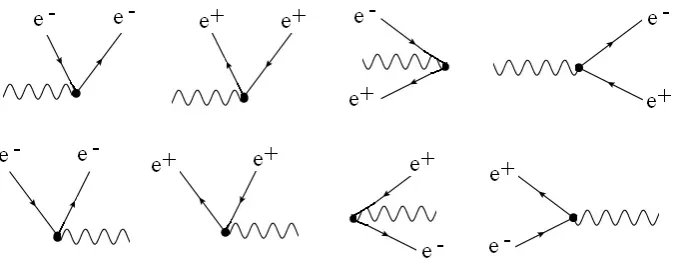
5.4. Example: Scattering in quantum electrodynamics 602
In quantum electrodynamics (QED), the operator equation for the creation and annihilation of the 603
field has the form (see [21]): 604
HW(x) =−eN{(ψ¯++ψ¯−)(6A++6 A−)(ψ+−ψ−)}x
605
whereψ+,ψ−, ¯ψ+, ¯ψ−,6A+,6A−are the creation and annihilation operators for electron, positron and
606
photon. This leads to the eight possible first order Feynman diagrams shown in Fig. 5. For a real
Figure 5.QED first order diagrams.
607
specific QFT scattering process, such as Bhabha scattering (e+,e−→e+,e−), the Feynman diagrams 608
are combinations of the appropriate first order diagrams. For Bhabha scattering this leads to the two 609
Feynman diagrams shown in Fig.6. 610
With QFT in position space, the vertexes of the diagrams shown in Fig.5and6can be associated 611
with space points. In the proposed model of spacetime, space points have associated connections to 612
their immediate neighbor space points. As described in Section 5.1, the propagation paths of QFT 613
(i.e., the lines of the Feynman diagrams) are mapped to the space point connections. As described in 614
Section 4.1, a typical space point has 14 connections. This enables different strategies for the mapping 615
of the three lines of the QED Feynman diagrams to the 14 space point connections. In Section 5.1 616
the overall strategy is described as the preservation of the number of fermion in-connections and 617
fermion-out connections and the allowance of additional boson connections. This enables the types 618
of QED space point connections shown in Fig. 7. 13. The cases that correspond to the QED first 619
order diagrams shown in Fig. 5are the cases (1) to (3). Case (4) and case (5) increase the diversity 620
12 For a given GSN, there may exist multiple repetitive states and a repetitive state may allow a range of values for specific
state components.
Figure 6.Feynman Diagrams for Bhabha Scattering.
of the possible fermion and boson paths. The more detailed strategy (i.e., algorithm) of the model
Figure 7.Possible QED connections of a space point.
621
determines (1) which of the connections of the space point are used as out connections, (2) which of 622
the out connections are fermion connections and (3) the distribution of attributes such as momentum 623
among the out connections. The respective algorithm contained in the present model is considered not 624
to be the final algorithm. Further experimentation by use of computer simulations is in progress. 625
6. Discussion
626
6.1. Local causal models, John Bell and David Bohm 627
The work described in this article is presented in the form of a causal model. The availability of 628
(or at least the feasibility of constructing) a causal model of an area of physics has been requested by 629
the author in many articles (see, for example, [3]). The introduction of the term "local causal model" 630
probably goes back to J. Bell when he formulated his famous Bell inequality and concluded that the 631
refutation of the inequality in experiments prohibits the creation of a local causal model of QT (see 632
[22]). It is probably not wrong to assume that J. Bell was convinced of the necessity of a (local) causal 633
model of QT. This would also explain his admiration of David Bohm (see [23]) whose search for a 634
deterministic model of QT may also be interpreted as the search for a causal model of QT (although 635
that conventional formulations of quantum theory, and of quantum field theory in particular, are 637
unprofessionally vague and ambiguous. Professional theoretical physicists ought to be able to do 638
better. Bohm has shown us a way." Although Bells inequality has been refuted in Aspects experiment 639
(see [24]) and Bohm’s interpretation of QT did not get many supporters among QT physicists, their 640
work and thinking influences QT physicists still until today with the attempts to overcome the many 641
ambiguities, vaguenesses, and non-localities still contained in QT. 642
The authors attempt to construct a local causal model of QT/QFT (and later of the dynamics of 643
spacetime) resulted in the experience that already, the attempt to construct a local causal model of an 644
area of physics may uncover weaknesses and vaguenesses of a theory (see [9]). In addition, the goal 645
of constructing a local causal model directs the selection of solutions towards specific solutions. For 646
example, the space-time relationship described in Section 3.1. and the Propositions 1, 2 and 3 are all 647
derived from the goal to construct a local causal model. 648
6.2. The special role of time 649
SRT and GRT have taught that space and time are integrated into spacetime. The major reason for 650
taking this view is that in the laws and equations of SRT and GRT, time and space occur in combination, 651
and the causal progression of the system state depends on the progression of the combination of both 652
space and time. The causal model of spacetime dynamics presented in this article also implies a tight 653
relationship of space and time, although with a different interpretation (see Section 3.1). 654
Nevertheless, there are also (good) reasons for not neglecting some fundamental differences 655
between space and time. The major points where the concept of time assumed for the model described 656
deviates from the time concept described (or implied) in some physics literature are: 657
• Arrow of time 658
The formal definition of a causal model (in general, not just for the model described in this 659
article) assumes a constant direction in which time progresses, i.e., an arrow of time. Reverse 660
progression of time or variable direction of time progression is just not supported by the model. 661
The author believes that a causal model in general implies an arrow of time. In other words, a 662
model that does not adhere to a unique constant direction of time would show more flexibility 663
than nature shows in reality. The model would not be reality conformal. 664
• Time slices 665
With the goal of showing as much commonality as possible between space and time, some 666
physics literature do not describe the extension of the time coordinate as differing from the 667
extension of the space. In the formal definition of a causal model, the laws of physics that specify 668
the state transitions can always access only the system state of the current point in time. It is not 669
possible to access past or future time slices of system states. Models that would allow reference 670
or even modifications of past or future system states are considered as (probably) not reality 671
conformal and would be very complicated. 672
6.3. Time dilation and/or length dilation? 673
Both SRT and GRT predict, under specific circumstances, time dilation and/or length contraction. 674
In textbooks covering SRT and GRT, it is not always clear whether (1) the two effects occur 675
simultaneously, (2) the two effects are just two possible views from a non-local observer, or (3) 676
there are cases where time dilation occurs (but no length contraction) and vice versa. For the proposed 677
model of spacetime dynamics, length dilation is the primary effect. In the model, time dilation - more 678
precisely, the clock rate dilation - is seen as a consequence of the length dilation. Length is a spatial 679
attribute, while clock rate is a property of processes running in a causal subsystem. (In areas of space 680
where there is no causal subsystem, there is no clock rate dilation, nor time dilation.) Despite the basic 681
differences in the roles that time dilation and length dilation play (in the model), these functions are 682
6.4. The general dependency of the clock rate on the length scaling 684
The model that assumes that GRT/SRT-based length dilations generally imply, as a secondary 685
effect, a proportional clock rate increase/decrease for the process that executes in the length-dilated 686
area of space requires a further non-trivial assumption. The additional rule is Conjecture 3.1 in Section 687
3.1: "All physical processes can ultimately be broken down to length-related state changes, and changes 688
in the length scaling, therefore, directly result in clock rate dilations of the affected process." 689
If it were possible to identify a process that is not accompanied by some spatial state change14, and 690
if it were possible to demonstrate that this process nevertheless adheres to GRT/SRT-predicted time 691
dilation, this would prove that the model that assumes that time dilation is always a consequence of 692
length dilation is wrong, or at least that it does not hold generally. The assumption that the rate of 693
state change of a clock process and of arbitrary other processes that show a regular rate of state change 694
depends in a predictable manner on the length scale of the space where the process executes is hard 695
to believe. If the assumption could be confirmed, it would indicate another, even tighter relationship 696
between time and space than is so far assumed with GRT. 697
6.5. The role of computer simulations 698
The development of the proposed causal model of spacetime and of QT/QFT has been 699
accompanied by extensive computer simulations. Especially in areas where the causal model requires 700
the determination of suitable algorithms computer simulations have been very useful. Mainly in 701
the following areas the task of determining suitable algorithms has been supported by computer 702
simulations: 703
1. The emergence of space from a single source with an increasing density of space points with 704
increasing distance from the gravitational source such that maximum compatibility with GRT is 705
provided (see Section 4.1). 706
2. The aggregation of space changes from multiple sources (see Section 4.2). 707
3. The assignment of in/out connections and of QFT particle types and particle attributes such that 708
maximum compatibility with QFT is provided (see Section 5.4). 709
In all three areas, the simulations resulted in useful findings.15 710
7. Conclusion
711
The model of spacetime dynamics and of QT/QFT described in this article does not aim at 712
providing another theory of the subjects. Rather, it has the goal of providing a special model, namely 713
acausal model, of these subjects for which a generally agreed upon theories exist. However, it is not 714
possible to derive a causal model of QT/QFT purely from existing QT/QFT. Nor is it possible to derive 715
a causal model of spacetime dynamics purely from GRT. QT/QFT and GRT establish a powerful base 716
for the development of the model, but supplementary statements and interpretations are required to 717
construct a somewhat complete (local) causal model of these areas of physics and their combination. 718
The described causal model is not claimed to be the only possible or valid model of the subjects. 719
Alternative models, possibly focusing on specific aspects, are imaginable. With those features of 720
the model that could not be directly derived from QT/QFT and/or GRT and where, therefore, new 721
solutions had to be invented, it may turn out that the solutions of the present model have to be replaced 722
by solutions that are in accordance with new experiments. 723
The two major items, where the proposed model deviates from the standard interpretations of 724
GRT and QFT are: 725
14 An example could be the decay of particles.
15 The author does not yet consider the computer simulations as closed. Further computer simulations may result in further
1. The assumption of the length dilation as the primary effect of space curvature that causes clock 726
rate dilation as a secondary effect. 727
2. The assignment of additional bosonic create operators for the out-connections of space points 728
(see Section 5). 729
Disregarding the uncertainties about the ultimate validity of certain details of the proposed model, 730
there are nevertheless a number of findings that the author believes are worth noticing: 731
• For an area of physics, it is mandatory that the construction of models of the complete dynamics 732
is feasible. The type of model that is best suited to describe the complete dynamics is the causal 733
model. The lack of feasibility of constructing a causal model of a theory of physics may be 734
considered as an indication of the incompleteness of the theory. 735
• As SRT and GRT show, space and time have to be viewed as integrated. The progression of time 736
can be described only in connection with spatial state changes. The length scaling within space 737
(including curvature) can only be described with reference to processes executing for a specific 738
time interval. However, besides this fundamental tight relation between space and time, it is also 739
necessary to point out the fundamental differences in the roles, structure, and properties of space 740
and time. 741
Further work is required to refine the model and make the ideas more solid. Dealing with discrete 742
space, time, and paths, refinements of the model may probably be achievable only with the help of 743
computer simulations. 744
Acknowledgments
745
I am grateful to the Fetzer Franklin Fund who covers the article processing charge for this article. 746
References
747
1. Diel, H.H. A model of spacetime dynamics with embedded quantum objects. Rep. Adv. Phys. Sci. (2017)
748
Vol. 1, No 3 1750010, https://doi.org/10.1142/S2424942417500104
749
2. Diel, H.H. Collective Behavior in a Local Causal Model of Quantum Theory. Open Access Library Journal ,
750
(2017) 4: e3898. https://doi.org/10.4236/oalib.1103898
751
3. Diel, H. Quantum objects as elementary units of causality and locality (2016), http://arXiv:1609.04242v1
752
4. Loll, R.; Ambjorn J.; Jurkiewicz, J. The Universe from Scratch (2005), http://arXiv:hep-th/0509010
753
5. Loll, R.; Ambjorn J.; Jurkiewicz, J. Reconstructing the Universe (2005), http://arXiv:hep-th/0505154
754
6. Ambjorn J.; Jurkiewicz, J.; Loll, R. Quantum Gravity, or The Art of Building Spacetime (2006),
755
http://arXiv:hep-th/0604212
756
7. Thiemann, T. Loop Quantum Gravity: An Inside View. Approaches to Fundamental Physics. Lecture
757
Notes in Physics. (2003) 721: 185–263.(2006) Bibcode:2007LNP...721..185T ISBN 978-3-540-71115-5.
758
https://doi.org/10.1007/978-3-540-71117-9-10
759
8. Rovelli, C. Loop Quantum Gravity Living Reviews in Relativity. 1. Retrieved 2008-03-13.
760
http://www.livingreviews.org/lrr-1998-1).
761
9. Diel, H. The completeness, computability, and extensibility of quantum theory, (2016)
762
http://arXiv:1512.08720
763
10. ’t Hooft, G. The Cellular Automaton Interpretation of Quantum Mechanics (2016) Springer,
764
https://doi.org/10.1007/978-3-319-41285-6
765
11. Elze, H-T. Are nonlinear discrete cellular automata compatible with quantum mechanics?, J. Phys.: Conf. Ser.
766
631, 012069, (2015) http://arXiv:1505.03764
767
12. Fredkin, E. Digital mechanics: An informational process based on reversible universal cellular automata,
768
Physica D 45, 254-270 (1990)
769
13. Diel, H. A Lagrangian-driven Cellular Automaton supporting Quantum Field Theory, (2015)
770
http://arxiv.org/abs/1507.08277
771
14. Schutz, B.F. A First Course in General Relativity, (2009) Cambridge University Press, New York
772
15. Wikipedia on "Real-World Relativity: The GPS Navigation System"