Bayesian genomic selection: the effect of haplotype length and priors

Open Access

Proceedings

Bayesian genomic selection: the effect of haplotype length and

priors

Trine Michelle Villumsen*

_{and Luc Janss}

Address: 1_{University of Aarhus, Faculty of Agricultural Sciences, Department of Genetics & Biotechnology, Research Centre Foulum. DK-8830, Box}

50, Tjele, Denmark and 2_{University of Copenhagen, Faculty of Life Sciences, Department of Large Animal Sciences, 1870 Frb. C., Denmark}

Email: Trine Michelle Villumsen* - [email protected] * Corresponding author

Abstract

Breeding values for animals with marker data are estimated using a genomic selection approach where data is analyzed using Bayesian multi-marker association models. Fourteen model scenarios with varying haplotype lengths, hyper parameter and prior distributions were compared to find the scenario expected to give the most correct genomic estimated breeding values for animals with marker information only. Five-fold cross validation was performed to assess the ability of models to estimate breeding values for animals in generation 3. In each of the five subsets, 20% of phenotypic records in generation 3 were left out. Correlations between breeding values estimated on full data and on subsets for the "leave-out" animals varied between 0.77–0.99. Regression coefficients of breeding values from full data on breeding values from subsets ranged from 0.78– 1.01. Single-SNP marker models didn't perform well. Correlations were 0.77–0.89 and predicted breeding values were biased. In addition the models seemed to over fit the genomic part of the variation. Highest correlations and most unbiased results were obtained when SNP markers were joined into haplotypes. Especially the scenarios with 5-SNP haplotypes gave promising results (distance between adjacent SNPs is 0.1 cM evenly over the genome). All correlations were 0.99 and regression coefficients were 0.99–1.01. Models with 5-SNP markers seemed robust to hyper parameter and prior changes. Haplotypes up to 40 SNPs also gave good results. However, longer haplotypes are expected to have less predictive ability over several generations and therefore the 5-SNP haplotypes are expected to give the best predictions for generations 4–6.

Introduction

We present an approach for genomic selection (GS) where the data is analysed using Bayesian multi-marker associa-tion models. The analysed data is the QTLMAS XII com-mon data set described in [1]. The aim is to get accurate genomic estimated breeding values (GEBV) for all

indi-viduals with marker information. We focus on how hyper and prior parameters and haplotype length affect the GEBV. A cross validation in generation 3 is used to evalu-ate the optimal model.

from 12th European workshop on QTL mapping and marker assisted selection Uppsala, Sweden. 15–16 May 2008

Published: 23 February 2009

BMC Proceedings 2009, 3(Suppl 1):S11

<supplement> <title> <p>Proceedings of the 12th European workshop on QTL mapping and marker assisted selection</p> </title> <sponsor> <note>Publication of this supplement was supported by EADGENE (European Animal Disease Genomics Network of Excellence).</note> </sponsor> <note>Proceedings</note> <url>http://www.biomedcentral.com/content/pdf/1753-6561-3-S1-info.pdf</url> </supplement> This article is available from: http://www.biomedcentral.com/1753-6561/3/S1/S11

© 2009 Villumsen and Janss; licensee BioMed Central Ltd.

Scenarios

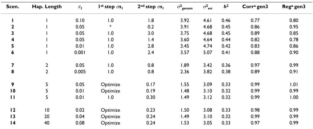
Fourteen scenarios were analysed. The models had haplo-type lengths of 1, 2, 5, 10, 20, and 40 SNPs. A two-mixture truncated normal distribution was used as prior for scal-ing factors that model the explained standard deviation per marker. We varied the proportion of markers to model the genetic effect and the prior parameter that determines the expected size of their scaling factors. The characteris-tics for each scenario are given in Table 1.

Analysis model

The model uses phenotypes and genotypes from all indi-viduals. Linkage phases of haplotypes are assumed to be known without error. The Bayesian model estimates allele

substitution effects at all m markers, with qi alleles at

marker i, as:

y = 1μ + Σ_i φ_i Σ_j x_ijβ_ij + e i = 1, m and j = 1, q_i

Here y is a vector of observations, μ is a general mean, xij

is a design vector indicating how many copies of the jth

allele of marker i are present in each observation, β_ij is the

allele substitution effect of the jth _{allele of marker i, and e}

is a vector of model residuals, e~N(0, Iσ_e2_{). Allele effects}

are modelled as random with β_ij~N(0,1) and φ_i is a scaling

factor that models the variance explained by ith _marker.

The scaling factor can be interpreted as a standard devia-tion. A Bayesian variable selection method utilises a prior mixture distribution to select if certain model compo-nents are included in the model. To implement a selection on the level of markers, we chose a prior mixture

distribu-tion on the scaling factor φ_i. The specification of the

remaining prior distributions is:

The prior mixture distribution for scaling factors φ_i follows

the Bayesian variable selection method proposed by [2]

where a large portion (π₀) of φ_i's is forced to come from a

distribution with small variance σs₀2_{, while only a small}

fraction (π₁ = 1 - π₀) of φ_i's is allowed to have big effects

coming from a distribution with large variance σs₁2_{. The}

model is augmented with mixture indicators γ= {γ_i},

indi-cating whether the ith _{scaling factor comes from the first}

component of the mixture (γ_i = 0) or from the second

component of the mixture (γ_i = 1).

Obtaining parameter estimates

A MCMC sampler was used to generate samples from the

joint posterior distribution of the model parameters f(μ,

φ, β, γ, σ_e2_{|y). The fully conditional distributions for} μ_, ϕ i's

and βij's are all Normal and the sampling of ϕi's is an

alter-nation between two two normal distributions. The

condi-tional posterior distributions of the mixture indicators (γ)

are Bernouilli [2] and the conditional posterior distribu-tion for residual variance is scaled inverse chi-square [3]. For all parameters single-variate Gibbs samplers were implemented. To obtain genomic predictions, MCMC chains were run in two steps. Aim of the first step was to

get a good estimate of the hyper parameter σs1. MCMC

chains for the full data were run with 10,000 cycles of which 3,000 burn-in; parameter samples were saved for

μ

Table 1: Starting parameters and estimates for the scenarios.

Scen. Hap. Length π1 1st step σs1 2nd step σs1 σ2genom σ2err h2 Corra gen3 Rega gen3

9 5 0.05 Optimize 0.17 1.55 3.09 0.33 0.99 1.01

10 5 0.01 Optimize 0.19 1.48 3.10 0.32 0.99 0.99

11 5 0.01 1.0 0.30 1.49 3.12 0.32 0.99 1.00

12 10 0.02 Optimize 0.23 1.50 3.08 0.33 0.98 0.99

13 20 0.04 Optimize 0.24 1.49 3.10 0.32 0.99 0.99

14 40 0.08 Optimize 0.24 1.53 3.05 0.33 0.97 0.99

each 100th _{cycle. In the second step GEBV were estimated}

with a fixed setting for σs₁ and leaving out certain

pheno-types (see "Cross validation" below). For the models with

haplotype length >= 5 the optimal σs₁ estimated from the

first step were used as known σs₁. For models with

haplo-type length 1–2, due to failure in estimating σs₁ at the first

step, best σs1 was assumed equal to the largest ϕi obtained

from the first step. MCMC chains were run with 10,000 cycles, of which 3,000 burn-in for haplotype length 1–2 and 5,000 cycles of which 2,000 burn-in for larger length of haplotypes.

Genomic predictions

GEBV were estimated for all individuals with marker information. The GEBV were constructed in each MCMC

cycle as functions of the scaling factors φ_i and allele effects

β_ij. Let x_ijE _{be extended versions of the design vectors with}

allele information for all individuals, then posterior

sam-ples of GEBV (g*) for all these individuals are:

g* = Σ_i φ_i* Σ_j x_ijE β ij*

where asterix (*) indicates samples from the posterior

dis-tribution. By constructing g as a function of joint (φ_i, β_ij)

samples within the MCMC, the covariances between φ_i

and β_ij are automatically taken into account, and also the

posterior standard deviations of g can be obtained. The

final estimate for GEBV is the posterior mean obtained as

the mean of a set of g* samples. Predictive abilities of

genomic prediction models were assessed as the correla-tion between GEBV from full data and GEBV from subsets for the "leave-out" animals.

Cross validation

To evaluate combinations of hyper parameter, prior distri-bution and haplotype length a five-fold cross validation was performed. In each of five data subsets phenotypic records were discarded for 2 out of 10 full sibs in genera-tion 3, equal to 300 discarded records in each subset. Each record was only discarded once, deleting the records for full sibs 1–2 in the first cross validation data set, the records for full sibs 3–4 in the second cross validation data set, etc. Assuming that ordering of full sibs is random within family; this is equivalent to a (stratified) random deletion of records. Only records in generation 3 were dis-carded, because this is closest to generations 4 to 6 where GEBV were estimated from marker information only. For each subset a genomic prediction was performed using

the same best estimate of σs₁ and number of cycles as for

the genomic prediction on full data. From each subset

GEBV of the 300 individuals with discarded phenotypic records were joined into a new dataset. This is called the "joined predicted" data. In the "joined predicted" dataset GEBV for all 1500 individuals in generation 3 were based on marker information only, because the GEBV for each

individual was retrieved from an analysis in which its own data was discarded.

For generation 3 correlations between GEBV from the full and joined predicted dataset and regression coefficient of GEBV from full data on GEBV from joined predicted data was computed. The best scenario is the one with highest correlation and the regression closest to one.

Results

Table 1 summarizes the starting parameters and the

esti-mates in 14 scenarios. For all scenarios σs0 is 0.01. The

sce-narios differ in haplotype length and in the settings for π₁

and σs₁ parameters, or in some cases included an

estima-tion of σs1 from the data. Genomic variance (σ2genom),

error variance (σ2

err) and heritability (h2) are presented.

The correlation between GEBV from full and joined pre-dicted data and the regression of GEBV from full data on GEBV from joined predicted data in generation 3 are also given.

For single marker models the correlations in generation 3 between GEBV obtained in full and joined predicted data are 0.77–0.89, highest for Scenario 3. For Scenario 2–4 the

only differences are in the setting of σs₁. The largest ϕ_i of

the markers was used as σs₁ in Scenario 3 while the second

largest was used in Scenario 4. In Scenario 2, a value close

to the automatic optimized σs₁ in the scenarios with

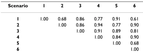
marker haplotypes was used to test if results were improved. The regression coefficient is 0.78–0.95, which indicates some bias. The lowest bias is found in Scenario 2. Table 2 shows that correlations between GEBV (for individuals in generation 3) obtained for full data in the six scenarios are 0.68–0.94, indicating that models are sensitive to prior and hyper parameter settings. The pre-sented single marker models do not perform well.

In the scenarios 7 and 8 with 2-marker haplotypes the

only difference is the setting of π1. The estimates of

vari-ances are different, but heritabilities are similar. Correla-tion and regression coefficients are higher than for single-SNP analyses. The correlation between GEBV from full data in the two scenarios is 0.96. The scenarios with 2-SNP haplotypes perform better than single-SNP models.

Table 2: Correlations of GEBV in generation 3 between scenarios for single-SNP models, based on full data.

Scenarios 9 to 11 with 5-SNP haplotypes perform simi-larly, independent of prior and hyper parameter settings.

Scenario 11 tests whether a large σs₁ (using the largest ϕ_i

from the first step) results in the same results as the

opti-mized σs₁. Variances and heritabilities are almost the

same, correlations and regression coefficients are almost one. In generation 3, the correlations between GEBV from full data in the three scenarios were all 0.99. The 5-SNP haplotypes fit data well and without bias, and is robust to changes in priors and hyper parameter.

Scenarios with 10, 20, and 40-marker haplotypes had

sim-ilar optimal σs₁, same variances and heritabilities.

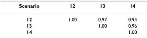
Corre-lations and regression coefficients are all close to one. All three models are expected to give good GEBV estimates. Table 3 shows that correlations between the GEBV esti-mated from the full data are 0.94–0.97.

Discussion

In this study we evaluated a Bayesian genomic prediction model with different grouping of SNPs into haplotypes and different settings of hyper and prior parameters. We assess the predictive abilities of the models using a cross validation in generation 3, assuming that the model which reached the best predictions in generation 3 would also be the model with the best predictions for genera-tions 4 to 6.

Single-SNP models did not perform well. As shown in the cross validation, the correlations for the single-SNP mod-els are the lowest observed among the given scenarios and the regression coefficients indicate bias. This was also found by [4]. Also the variance components in the single SNP models indicate bias and incorrect fitting of the data, with larger genomic variance and larger residual variance. This indicates that there must be a negative covariance between genomic fits and residuals, which is a sign of over fit. Overall, the single SNP models appeared variable and difficult to setting optimal prior and hyper parameter. We show that results from the single SNP model are relatively sensible for the prior and hyper parameter settings, and

estimation of the hyper parameter σs₁ from the data also

failed for the single SNP models, probably due to colline-arity between SNPs. A possible explanation for poor per-formance of the single-SNP model is that markers may not be in complete linkage disequilibrium with a QTL. In

order to improve the single SNP model, probably lower

settings for the σs₁ parameter are needed.

Models based on haplotypes of 5 SNPs and more gave much better results. For these models, regressions indi-cated absence of biases and estimates of variance compo-nents were better: residual variance was smaller, which indicates a better model fit, and the total fitted variance was close to the raw variance in the trait. In these models there is no numerical problem in estimating parameter

σs₁ from the data. Using the σs₁ estimated from the data is

expected to give accurate and unbiased predictions.

Models based on 5-marker haplotypes are expected to give the best estimates of GEBV in generation 4–6. In the eval-uation shown here the 10 to 40-SNP models perform equally well, but it should be noted that this is based on predictions in generation 3. For predicting breeding val-ues in generations 4–6, however, these larger haplotypes may lose predictive ability quicker as shown by [4]. There-fore we expect the 5 SNP haplotypes to retain the best pre-dictive ability over the generations 4–6. For estimation of GEBV in generation 4–6, Scenario 11 performs best with a correlation on 0.99 and a regression of exactly 1.00. GEBV from Scenario 11 are submitted for the workshop.

For scenario 11 the correlation between GEBV and true breeding value (TBV) in generation 4–6 turned out to be 0.92; the regression of TBV on GEBV from the full data was 0.98 indicating a small overestimation of GEBV. The

amount of variance in TBV explained by GEBV, R2 _was

0.84. Hence, the selected model predicted the data well and gave nearly unbiased GEBV. The results can be found in table 2 in [1].

The better results here from using haplotypes than single-SNP is different from [5] in which IBD probabilities between haplotypes were used and where the use of such haplotypes gave similar results as the use of single SNPs. All results are in table 2 in [1]. There are however a number of differences between our approach and [5] in the use of Linkage and Linkage Disequilibrium (LD) pos-sibly resulting in differences in the use of population-wide and family-specific effects. Our results show that signifi-cant improvements can be made from using haplotypes and that it is worthwhile to further investigate the use of haplotypes for making genomic predictions.

Conclusion

We expect the most correct GEBV to be estimated in Scenario11, because the correlation between full and joined data is 0.99 and the regression coefficient is 1.00. The haplotype models perform better than single-SNP models and are less sensitive to prior and hyper parameter settings.

Table 3: Correlations of GEBV in generation 3 between scenarios for 10, 20 and 40-SNP models, based on full data.

Scenario 12 13 14 12 1.00 0.97 0.94

13 1.00 0.96

Publish with BioMed Central and every scientist can read your work free of charge

"BioMed Central will be the most significant development for disseminating the results of biomedical researc h in our lifetime."

Sir Paul Nurse, Cancer Research UK

Your research papers will be:

available free of charge to the entire biomedical community

peer reviewed and published immediately upon acceptance

cited in PubMed and archived on PubMed Central

yours — you keep the copyright

Submit your manuscript here:

http://www.biomedcentral.com/info/publishing_adv.asp

BioMedcentral

List of abbreviations used

GEBV: genomic estimated breeding values; GS: genomic selection; TBV: true breeding value.

Competing interests

The authors declare that they have no competing interests.

Authors' contributions

TMV carried out the analyses and drafted the manuscript. LJ helped to draft the manuscript and to interpret and present the results in the manuscript. Both TMV and LJ read and approved the final manuscript.

Acknowledgements

This article has been published as part of BMC Proceedings Volume 3 Sup-plement 1, 2009: Proceedings of the 12th European workshop on QTL mapping and marker assisted selection. The full contents of the supplement are available online at http://www.biomedcentral.com/1753-6561/ 3?issue=S1.

References

1. Lund MS, Sahana G, de Koning D-J, Carlborg Ö: Comparison of analyses of the QTLMAS XII common dataset. I: Genomic selection. BMC Proceedings 2009, 3(Suppl 1):S1.

2. George EI, McCulloch RE: Variable selection via Gibbs sampling.

J Am Stat Assoc 1993, 88:881-889.

3. Sorensen D, Gianola D: Likelihood, Bayesian, and MCMC Methods in Quantitative GeneticsSpringer, New York, NY, USA; 2002.

4. Villumsen TM, Janss L, Lund MS: The importance of haplotype length and heritability using genomic selection in dairy cat-tle. J Anim Breed Genet 2008 in press. Published online: 24 Sep 2008; doi 10.1111/j.1439-0388.2008.00747.x