Copyright2000 by the Genetics Society of America
Bayesian Analysis of Response to Selection: A Case Study Using
Litter Size in Danish Yorkshire Pigs
D. Sorensen,* A. Vernersen
†and S. Andersen
†*Danish Institute of Agricultural Sciences, DK-8830 Tjele, Denmark and†National Committee for Pig Production, Axelborg, DK-1609 Copenhagen, Denmark
ABSTRACT
Implementation of a Bayesian analysis of a selection experiment is illustrated using litter size [total number of piglets born (TNB)] in Danish Yorkshire pigs. Other traits studied include average litter weight at birth (WTAB) and proportion of piglets born dead (PRBD). Response to selection for TNB was analyzed with a number of models, which differed in their level of hierarchy, in their prior distributions, and in the parametric form of the likelihoods. A model assessment study favored a particular form of an additive genetic model. With this model, the Monte Carlo estimate of the 95% probability interval of response to selection was (0.23; 0.60), with a posterior mean of 0.43 piglets. WTAB showed a correlated response of ⫺7.2 g, with a 95% probability interval equal to (⫺33.1; 18.9). The posterior mean of the genetic correlation between TNB and WTAB was ⫺0.23 with a 95% probability interval equal to (⫺0.46; ⫺0.01). PRBD was studied informally; it increases with larger litters, when litter size is⬎7 piglets born. A number of methodological issues related to the Bayesian model assessment study are discussed, as well as the genetic consequences of inferring response to selection using additive genetic models.
O
VER the last years, pig breeding programs have size was based on results of hyperprolific designs(BichardandSeidel1983;TomesandNielsen1984; emphasized selection pressure on fertility traits.
While it is recognized that fertility is a composite trait, Legault1985). With the exception of results from
Ne-most of the efforts to improve sow reproductive perfor- braska published in the 1990s, which focused on
improv-mance have been placed on selection for litter size. This ing litter size by selecting on an index that included
is partly because litter size is easily recorded and partly ovulation rate and embryo survival (Caseyet al.1994),
because several studies have indicated that it is the most all other attempts to increase litter size in pigs by direct
important economic component of sow reproductive selection produced unconvincing results (see reviews
performance (Bichard et al. 1983;Smith et al. 1983; by Blasco et al. 1995 and Rothschild and Bidanel
Tesset al.1983). 1998).
There is a substantial amount of information in the Against such a background, it was decided in the late
literature about genetic parameters for litter size in pigs; 1980s to generate convincing experimental evidence
much of this has been reviewed byHaleyet al.(1988) that litter size could be improved by selection. The
crite-and more recently byRothschildandBidanel(1998). rion of selection should be inexpensive and simple to
RothschildandBidanel(1998) quote an average fig- measure and the choice fell on total number of piglets
ure of heritability for total number of piglets born per born per litter. A large-scale selection experiment was
litter, over 85 published results, of 0.11, with a range conducted from 1989 to 1992. The experiment’s results
from 0.0 to 0.76. Using this average figure, and assuming have been reported on occasion (Blasco et al.1995),
a value for repeatability over several parities of 0.15, but a formal investigation of the data, with the most
up-predicted rates of genetic improvement range from to-date methods of inference, has not yet been
pub-ⵑ0.3 to 0.5 pigs per litter and generation, depending on lished.
the amount of information included to predict breeding This article is an attempt to fill in this lack. The
empha-values (A´ valos and Smith 1987). These calculations sis of this work is on the methodological aspects of the
are based on the infinitesimal model and assume infinite analysis. Over the last years, with the introduction of
population size and in the late 1980s stimulated a reex- Markov chain Monte Carlo (MCMC) techniques, there
amination of the possibilities for genetic improvement has been a revival of Bayesian methods in the statistical
of litter size. At that time, the only experimental evi- literature, and geneticists have been receptive to the
dence for successful direct selection for increased litter inferential possibilities that the Bayesian paradigm
of-fers. This article illustrates the type of information that can be extracted from a selection experiment when Corresponding author:Daniel Sorensen, Danish Institute of
Agricul-MCMC is used in combination with the Bayesian
ap-tural Sciences, Department of Animal Breeding and Genetics, P.O.
Box 50, DK-8830 Tjele, Denmark. E-mail: [email protected] proach.
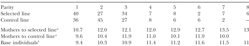
TABLE 1
Distribution of the number of sows across parities among 261 female parents of animals inselected
andcontrollines (top three lines) and raw means of total number of piglets born per litter, within parity and line (bottom three lines)
Parity 1 2 3 4 5 6 7 8
Selected line 40 27 34 7 8 2 7 6
Control line 36 45 27 8 6 6 2 —
Mothers to selected linea 10.7 12.0 12.1 12.0 12.9 12.7 13.5 13.0
Mothers to control linea 9.6 10.4 11.9 11.0 10.1 11.9 10.0
Base individualsb 9.4 10.3 10.9 11.4 11.2 11.6 11.5 11.4
aThe 261 female parents of selected and control lines.
bThe 3534 females with records on 8988 litters, excluding data from selected and control lines.
EXPERIMENTAL DESIGN AND DATA immediately after weaning at 17–23 days of age. On
arrival at the common farm, the piglets underwent a The data originate from the database of the national
period of quarantine in a nursery. breeding program. Litter size (total number of piglets
At the common farm, females of each line were ran-born per litter) had been recorded in the breeding
domly mated (mating took place after the second oes-herds, even though it had not been part of the breeding
trus) with males of the corresponding line and pro-goal. In 1989, the large-scale selection experiment was
duced two parities. These are records fromgeneration 1.
started using data from the Yorkshire breed only.
Infor-From the first of these two parities, one gilt was chosen mation on litter size was gathered from all matings in
from each litter. At sexual maturity, these females were the breeding herds, and predicted breeding values for
mated twice to randomly chosen males from the appro-each mating were computed using a model that is
de-priate line and produced, therefore, two litters. We refer scribed below.
to these as the records fromgeneration 2.There was no
The data set used to compute predicted breeding
directional selection to produce litters in generation 2, values was produced as follows. On the basis of the
but the genotypic value of these females is expected to matings available during an 8-month period, records
be a little higher than those from generation 1, because on ancestors and collateral relatives were generated and
their 36 fathers represent a smaller proportion of the updated each month. This data file consisted of records
tail of the distribution than the fathers to females from from 8988 litters and a total of 5796 animals, of which
generation 1. 3534 were females with records. These animals are
re-In total, there were 1072 litters in the common farm,
ferred to simply as the base. The pedigree of this file
approximately equally distributed between the selected included animals born from 1981 until 1988.
and the control lines. The total number of litters in the During the period of 8 months, from the highest
complete data set was 10,060 (8988 from the base plus scoring 131 predicted breeding values of the registered
1072 from the selected and the control lines) and the matings, 1 gilt was chosen from each resulting litter,
total pedigree file consisted of 6437 individuals (5796 and from the highest scoring 36 predicted breeding
from the base and 641 from the selected and the control values, 1 male piglet was chosen from each resulting
lines). litter. These 131 gilts and 36 male piglets constituted the
Animals from both lines were kept under identical
selected line.A contemporaneouscontrol linewas created,
conditions and it was not possible for the staff in the choosing 130 gilts and 38 male piglets at random from
farm to identify to which line animals belonged. As the litters available. Selection took place on a monthly
customarily practiced in the breeding herds, litters in basis, during 8 months, and not just once at the end of
the common farm were also standardized at birth ac-the 8-month period. Table 1 shows ac-the contribution of
cording to total number of piglets born. The traits re-the different parities to re-the 261 sows from re-the selected
corded on the farm were total number of piglets born and control lines, as well as the raw means of total
per litter (TNB), number of piglets born alive per litter number born per litter of the mothers of these 261
(NBA), and average weight of liveborn piglets (WTAB). sows, within parity and line, and among the 3534 females
The latter was recorded within 24 hr after birth; the that belong to the base. The weighted average of the
whole litter was weighed, rather than individual piglets. difference across parities of records on females that
Among the 6437 individuals in the pedigree file, 3537 contributed piglets to the contemporaneous selected
had an inbreeding coefficient ⬎0.0. The average
in-and control lines is 1.6 piglets per litter.
breeding coefficient among inbred individuals was Animals from both lines were purchased from the
maxi-mum value was 32%. Only 88 inbreeding coefficients the availability of litter weights, rather than of individual piglet weights.
were⬎10%.
Selection criterion—model for prediction of breed- The analyses of TNB were done by fitting two types
of models that differ fundamentally in the way data
ing values:The data available on litter size before the
contribute to infer response to selection. The first type selection experiment was initiated consisted of records
is a nonhierarchical model, where only data that belong on TNB only. The criterion of selection was the average
to a generation in question contribute to infer the ge-predicted breeding value of the sire and dam of the
netic mean of that generation. The second type is repre-litter that contributed piglets to the selected and control
sented by hierarchical additive genetic models, where lines. The model was a repeatability additive genetic
the complete data contribute information to the genetic model and the method of inference was best linear
mean of a particular generation, leading to sharper
unbiased prediction (BLUP; i.e., Henderson 1973).
inferences. This is at the expense of a higher level of Thus, the variances of the random effects were assumed
parameterization and stronger assumptions about the known and the values used for these parameters were
form of gene action. those traditionally quoted in the literature at the time
Single-trait analyses of TNB: Nonhierarchical model:
(Haleyet al. 1988): 10% for heritability and 15% for
The simplest model entertained is one that ignores the repeatability. The model included, as fixed effects,
herd-family structure in the data. This is labeled the nonhier-year-type of insemination (artificial insemination or
archical (NH) model, in contrast with the additive ge-natural service), season, and parity; as random effects,
netic models described below. The NH model consid-additive genetic values and permanent environmental
ered here assumes the following relationship between effects. The vector of additive genetic values was
as-the dependent variable and as-the parameters, sumed to follow a multivariate normal distribution, with
zero mean and with variance equal toA2
a, whereAis y
ijklm⫽li⫹pj⫹gk⫹sl ⫹eijklm,
the additive genetic relationship matrix among all
i⫽1, 2;j⫽1, 2;k⫽1, 2;l⫽ 1, . . . 4, (1)
breeding values in the data, and2
ais the additive genetic
variance. The vectors of permanent environmental ef- where y
ijklm is a record (TNB) from line i (li), parity j
fects and residual effects were assumed to follow normal (p
j), generation k(gk), and seasonl(sl). Data from the
distributions with zero mean, and with variances I2
p common farm only (selected and control lines) are
in-andI2
e, respectively, where2pdenotes the variance due cluded in the analysis. Response to selection is defined
to permanent environmental effects and2
eis the resid- as
ual variance. These three random vectors were assumed
R1⫽l1⫺ l2, (2)
to be mutually independent.
The design used in the experiment was chosen on
which is the difference between the effects of the se-the basis of previous calculations using se-the above model.
lected and control lines and which is inferred from its
These calculations indicated a predicted deviation be- marginal posterior distribution. In (2), no distinction
tween selected and control line of 0.49 piglets per litter. is made between responses at generations 1 and 2. A
With the experimental design implemented, the ap- model similar to (1), which included instead
line-by-proximate probability of detecting such a deviation was generation interaction effects, did not reveal a
differ-estimated as 71%. ence between the responses at generations 1 and 2, and
the results of this analysis are therefore omitted. Model (1) is written in matrix form as
STATISTICAL METHODS
y⫽Xb⫹ e, (3)
The main objective of this experiment has been to
where b is the vector that has parameters associated
confirm that litter size (TNB) responds to selection in
with line, parity, generation, and season, andXis the
the Danish Yorkshire breed. To address this concern, a
known incidence matrix. It is assumed thaty|b is
nor-number of single-trait analyses of TNB were performed
mally distributed, with mean and variance equal toXb
using a variety of models. The experiment also generates
andI2
e, respectively. A priori, the vector b ⫽ {bi} is
as-data to study correlated responses in proportion of
pig-signed a 10-dimensional uniform distribution, indepen-lets born dead (PRBD) and average piglet weight at
dent of the residual variance; the latter is assumed to birth, although it was not specifically designed to
ad-be proportional to 1/2
e. Therefore,
dress these questions. Correlated responses in WTAB were analyzed using two-trait models only; PRBD was
p(b,2 e)⬀
1
2 e
,⫺∞⬍bi⬍ ∞, for all i; 0⬍ 2e⬍∞.
analyzed only informally. Most of the analyses were car-ried out within the Bayesian framework of inference.
In the analyses presented below, TNB and WTAB are With the present choice of prior distributions, the
mar-both regarded as traits of the mother of the litter. In ginal posterior distribution of selection response
(de-fine selection response asR⫽kⴕb) follows a univariate
t-distribution with mean equal toE(R|y)⫽kⴕ(XⴕX)⫺1Xⴕy, a|A,2
aⵑ N(0,A2a) (5)
scale parameter equal toˆ2
ekⴕ(XⴕX)⫺1k, and with degrees
p|2
pⵑ N(0,I2p). (6)
of freedom equal ton ⫺rank(X), where
In these expressions,2
ais the additive genetic variance
ˆ2
e⫽(y⫺ Xbˆ)⬘(y⫺Xbˆ)/(n⫺rank(X))
in the population from which individuals with unknown
parents were conceptually sampled, and2
pis the
perma-andn is the number of elements iny(BoxandTiao
1973). The marginal posterior distribution of 2
e is a nent environmental variance. The matrixAhas, as
ele-ments, additive genetic relationships among the genetic scaled inverted chi-square distribution with scale
param-eter (n⫺rank(X))ˆ2
eand (n⫺rank(X)) d.f. Note that values.
The models differed in their prior distributions and in
the mean of [R|y] is numerically identical to the
least-squares estimator. the specification of the herd-year-type of insemination
effects. In model 1, vectorbhas effects of herd-year-type
Hierarchical models via Markov chain Monte Carlo:
Hier-archical models include a number of additive genetic of insemination, season, and parity. A priori, variance
components are assumed to be independently and uni-models that were fitted using the Gibbs sampler. With
the additive genetic models, response to selection at formly distributed, taking values in the following ranges:
0 ⬍ 2
a ⱕ 4, 0 ⬍ 2p ⱕ 2, and 0 ⬍ 2eⱕ20. These
generation 1 is defined as the difference in the average
additive genetic values between individuals from the distributions for the variance components imply an a
priori distribution of heritability and repeatability with selected line, generation 1, and those from the base.
This is labeledR1. Response to selection at generation respective modal values of 0.15 and 0.23 (Sorensen
1996). 2 is correspondingly defined as the difference in the
average additive genetic values between individuals Model 2 differs from the above in that the vector of
herd-year-type of insemination effects,h, is assumeda
from the selected line, generation 2, and those from
the base. This is labeled R2. priori, to follow a multivariate normal distribution:
An alternative expression of response to selection
in-h|2
hⵑ N(0,I2h). (7)
volves deviating the mean additive genetic value of the
offspring of selected parents from the average additive The vectorbnow contains effects of parity, season, and
type of insemination (artificial vs. natural service). All
genetic values of all matings available during the
8-month period (the group from which parents were variance components (2
a,2h,2p,2e) are assumed to be
a priori, independently and uniformly distributed, taking chosen). However, since TNB shows no genetic trend
over the period studied (not shown) and the mean of values in the ranges described above. For2
h, the range
was 0⬍ 2
hⱕ2.
the posterior distribution of the average additive genetic
values of the base is smaller than 10⫺4, the above defini- Finally, response was also evaluated using a model
similar to model 1, except that heritability and repeat-tion was chosen. Note that with the additive genetic
model, response to selection is not defined as a deviation ability were assumed to take values 0.10 and 0.15,
respec-tively, and the posterior distribution of response was involving the control line.
The initial model choice was based partly on the work obtained, conditional on these values. This is denoted
model 3 and is the same model used to carry out selec-of Estany and Sorensen (1995). In their analysis of
litter size, using a larger data set that included data from tion decisions and is numerically equivalent to a BLUP
approach if heritability and repeatability are the true 1978 to 1989, it was shown that neither group effects
nor maternal effects contributed to variation in litter values. In a frequentist setting, the sampling variance
of the “BLUP estimate of selection response” must be size in Danish Yorkshire. With this information as a
background, three single-trait models were fitted to the computed over the distribution of the selected data;
this is not an analytically tractable task. The Bayesian complete data set. For the three models, it is assumed
that the data vector containing records on TNB (y) is analysis implemented here via the Gibbs sampler yields
a measure of uncertainty associated with selection re-conditionally normally distributed as
sponse in the form of a Monte Carlo estimate of the
y|b,a,p,2
eⵑN(Xb⫹Za⫹Wp,Ie2), (4) posterior variance.
Two other models were also fitted: one of these
dif-where b is a vector that contains location parameters
whosea prioridistributions are assumed to be uniform, fered from model 1 in the a priorispecification of the
variance components. These were assumed to follow
with lower and upper bounds equal to bmin and bmax,
respectively, andaandpare vectors that contain addi- scaled inverted chi-square distributions, reflecting little
information about the variance components. The other tive genetic values and permanent environmental
ef-fects, respectively. MatricesX,Z, andWare known inci- model differed from model 2 in the same way. The first
of these two behaved almost identically to model 1, and
dence matrices, and2
eis the residual variance.A priori,
it is assumed that additive genetic values and permanent the second one behaved almost identically to model 2.
Therefore, results obtained from these two models are environmental effects are multivariate normally
The boundsbminandbmaxwere set equal to 0 and 20, theoth dam effect, assumed normally distributed, with
mean zero and variance2
d; andApis thepth sow effect,
respectively, for all elements in eitherbminor bmax, for
all models. Runs with different bounds yielded almost assumed normally distributed, with mean zero and
vari-ance 2
a. A similar model with a regression coefficient
identical results and these are therefore not presented.
Two-stage regression of TNB on parental predicted additive for each of the two lines was also fitted to the data, but no difference could be detected between the two
regres-genetic values:The data were analyzed also using a
two-stage approach, designed to study whether TNB sion coefficients.
Two-trait analysis of TNB and WTAB: As with the
achieved after selection was consistent with predictions
based on the additive genetic model 1 (Andersenet al. single-trait analyses, a number of two-trait models were
investigated. The models differed in the form of the 1998). In a first stage, data from the base only (excluding
data from selection and control lines in the common prior distributions and in the covariance structure of
location parameters. Inferences about response to selec-farm) were used to obtain estimates of genetic variances
and additive genetic values. In a second stage, using only tion for TNB and correlated responses in WTAB were
almost identical in all cases; we present, therefore, re-the data from selection and control lines, generation 1,
the following model was fitted to TNB, sults from the most parsimonious among the models
studied.
yijkl⫽ti ⫹sj⫹ pedk⫹ f,k⫹ m,k⫹ pk⫹ eijkl, (8) Let (y, z) denote the vector of length 10,060 ⫻ 2
representing the n ⫽ 10,060 records on TNB (vector
wheretiis the effect of theith parity,sjis the effect of the
y), and the augmented WTAB data (z). The latter was
jth season, pedk⫽(aˆf,k⫹aˆm,k)/2, the average predicted
augumented with 10,060⫺1072⫽8988 missing
residu-additive genetic values of the father and mother of sow
als. It is assumed that theith record (yi,zi) is
condition-kbased on the first stage analysis,f,k⫽(af,k⫺aˆf,k)/2 and
ally, bivariate normally distributed, given the parameters
m,f,k⫽ (am,k⫺ aˆm,k)/2 are random errors of prediction
associated with the father (f) and mother (m) of k,pk
冢冤
yizi
冥
兩
by,bz,py,pz,ay,az,Rei
冣
ⵑ N冢冤
x⬘iyby⫹wiy⬘py⫹ z⬘iyay
x⬘izbz⫹ w⬘izpz⫹ z⬘izaz
冥
,Rei
冣
,is the sum of the effects of Mendelian sampling and
permanent environmental effects, andeijklis a residual
effect peculiar to thelth record. Note that no distinction i ⫽1, . . . ,n, (10)
is made between records from selection or control lines.
whereRei, is theith residual covariance matrix, which
If TNB does not respond to selection, it is expected that
has the structure
 ⫽ 0; under the assumption that the model holds,
 ⫽1. This analysis was carried out using a frequentist
approach. Rei⫽ iRe⫽
冤
1 0
0 1/ni
冥 冤
2 ey
eyz
eyz
2 ez
冥
. (11)
Single-trait analysis of PRBD: Data on PRBD were
markedly skewed and it was not possible to find a trans- In (11),niis the known number of records contributing
formation to remove this skewness. A formal analysis to WTAB. Elements of the row vectors x⬘i, w⬘i, and z⬘i
of the correlated response in PRBD, which requires (subscriptsyandzrefer to TNB and to WTAB,
respec-inclusion of the trait selected for TNB, will be presented tively), associated with a missing residual, contain only
in the future. At this stage, we report results from a zeroes. The vectorb has location parameters that are
univariate analysis based on the approach inKerrand assumed to be uniformly distributed,a priori.For both
Cameron(1995). TNB is considered as fixed, and NBA TNB and for WTAB, these are herd-year-type of
insemi-is modeled using a generalized linear mixed model with nation effects, season, and parity. The vectors py and
binomial errors and a probit link function of the bino- pzrepresent permanent environmental effects and the
mial probability PRBD. vectorsayandazrepresent additive genetic values.
Addi-It was cursorily observed that PRBD increases when tive genetic values and permanent environmental
ef-TNB is⬎7. Therefore, the following phenotypic rela- fects are assumed to be,a priori, multivariate normally
tionship was studied between PRBD and TNB, distributed:
Probit(PRBDijklmnop)⫽li⫹pgj⫹sk⫹tl⫹ TNBpI(TNBp⬎7)
冤
ayaz
兩
Go,A
冥
ⵑ N冢冤
0
0
冥
, [Go丢A]冣
⫹Sn⫹Do⫹Ap, (9)
where li is the effect of linei (i ⫽ 1, 2);pgj is thejth
冤
pypz
兩
2
py,2pz
冥
ⵑN冢冤
0 0
冥
,冤
Imp2y
0 0 Im2pz
冥冣
.
interaction effect of parity by generation;skis the effect
of season k; tl is a classification variable that takes the
In these expressions,Gois the 2 by 2 matrix of additive
value TNB if TNBⱕ 7 and zero otherwise; I(TNBp⬎
genetic variances and covariances, and2
pyand
2 pzare
7) is the indicator function that takes the value 1 if the
argument is satisfied and zero otherwise;is a regres- the variances due to permanent environmental effects
associated with TNB and WTAB, respectively.
sion coefficient; Snis the nth sire effect assumed
nor-mally distributed, with mean zero and variance2
improper uniform prior distributions, a priori.This is in Geyer(1992). This is used as a criterion to decide whether differences among estimates of posterior
denoted model 4. In model 5, for TNB, herd-year-type
of insemination effects were assumed to have, a priori, means from different chains can be attributed to
sam-pling variation. Plots of histograms of samples from independent normal distributions, with zero means.
In-dependent scaled inverted chi-square distributions were posterior distributions were also compared among runs,
to confirm consistency of results. When the total length
assigned to2
pyand to2pz(and to2hy), and scaled inverse
of the chain approached 100,000 and the burn-in period
Wishart distributions toGoandRe. The parameter
“de-was 10,000, runs from different chains within models grees of freedom” associated with all these distributions
yielded practically identical results. We present numbers
was set equal to 5. This is intended to reflect weak a
based on final runs using chains of length 500,000 with
priori information. Variants of the above models with
a burn-in period of 50,000. These numbers exceed, by respect to prior specifications were also fitted, with
a factor of 100, those suggested using the criterion of hardly any consequences on inferences about response
Raftery and Lewis(1993). The value of the statistic and correlated response to selection. Therefore, results
proposed by Gelman and Rubin (1992) was never
based on only models 4 and 5 are shown.
⬎1.18 (when this statistic is equal to 1.0, the chains are
The first step in the implementation of the Gibbs
essentially overlapping). Among the estimates shown, sampler was the generation of the WTAB missing
residu-the effective chain size (Sorensenet al.1995) for
infer-als from the fully conditional posterior distribution.
ences about selection response was never⬍1900. The
From (10), this has the form
estimates of the Monte Carlo standard error for the
zm,i|yo,i,b,p,a,ReⵑN(E(zm,i|yo,i,b,p,a,Re), Var(zm,i|yo,i,b,p,a,Re)), different expressions of selection response were of the
order of 0.0025. The corresponding estimates for herita-where
bility, repeatability, and proportion of variance due to
herd-year-type of insemination effects are⬍0.0004.
E(zm,i|yo,i,b,p,a,Re)⫽ e,yz
2 e,y
(yo,i⫺x⬘yo,iby⫺w⬘yo,ipy⫺z⬘yo,iay)
It was estimated that the large proportion of missing data could cause very slow mixing. Therefore, after aug-and
menting with the missing residuals, the sampler was implemented using a multiple-trait extension of the ap-Var(zm,i|yo,i,b,p,a,Re)⫽ 2e,z(1 ⫺re,2yz).
proach suggested by Garcia-Cortes and Sorensen
In these expressions,zm,irepresents theith missing resid- (1996); rather than sampling each location parameter
ual,yo,iis theith TNB observation,x⬘yo,i,w⬘yo,i, andz⬘yo,iare scalarly, all the location parameters are sampled jointly,
the rows ofXy,Wy, andZyassociated withyo,i,e,yzis the in one pass.
residual covariance between TNB and WTAB,2
e,z(2e,y) Evaluating contributions to statistical information
is the residual variance associated with WTAB (TNB), about response to selection:It is of interest to quantify
and re,yz⫽ e,yz/
√
2e,2e,y is the residual correlation be- the relative amount of information contributed bysub-tween traits. After generating the augmented data, loca- sets of the data to the posterior distribution of selection
tion parameters were sampled from the appropriate response. To achieve this, response to selection is
stud-multivariate normal distribution, variances were sam- ied using two types of analyses. In the first one,
pheno-pled from the appropriate fully conditional inverse chi- typic records from the selected and control lines
(la-square posterior distributions, and covariance matrices beled vectory2) are excluded; only data from the base
from the appropriate scaled inverse Wishart distribu- (labeledy1) contribute to inferences about response to
tions. Each iteration required generation of a new set selection. This is denoted thepredictive analysis.Since the
of missing residuals and the construction of the mixed- additive genetic models assume that parental additive
model equations. Further details of the algorithm can genetic values combine additively to generate the
addi-be found, for example, inSorensen(1996). tive genetic values in their offspring, and since the
pedi-Gibbs sampling implementation: The results pre- gree is known, selection response can be inferred using
sented below are based on Monte Carlo estimates of y1 only. In a second analysis, the complete data,yⴕ ⫽
means of posterior distributions. A large number of (y⬘1,y⬘2), are included to draw inferences; this is the
com-experiments for each model were run with the Gibbs plete data analysis.
sampler. The burn-in periods and number of iterations Let represent the vector of parameters for a given
of the various Gibbs chains were chosen partly pragmati- model and letp() denote the prior distribution of.
cally, looking at the results of various independent Then the posterior distribution of, conditional on the
chains as time-series plots overlaid and seeing if these complete data, is given by
could be distinguished, and partly using more formal
p(|y1,y2)⬀p()p(y1,y2|)
methods. These include the approaches ofGelmanand
Rubin(1992) and ofRafteryandLewis(1993). Monte ⫽ p()p(y
1|)p(y2|), (12)
Carlo sampling errors of features of posterior
models considered here,y1andy2are conditionally
inde-pˆ(y|Mi)⫽
冤
1
m
兺
j⫽m j⫽1
p⫺1(y|(j)
i ,Mi)
冥
⫺1
. (15)
pendent, given. The predictive analysis is associated
with the first two terms in the right-hand side of (12).
In (15),(j)
i represents thejth Gibbs sample fromp(i|y,
Taking logarithms, and differentiating twice with
re-Mi) andmis the total number of samples drawn. The
spect to, yields
marginal likelihood can be interpreted as the
probabil-I(|y1,y2)⫽I()⫹ I(y1|)⫹I(y2|). (13) ity of obtaining the data actually observed under model
i, calculated before any data became available (Kass
Equation 13 shows that the amount of information in
andRaftery 1995). It is thus a global measure of the the posterior distribution is equal to the sum of
informa-model’s ability to explain the observed data.
tion contributed by the prior distribution,I(), by the
We are also interested in studying how the models
sampling model of the base,I(y1|), and by the sampling
predict specific features of the data. Since the scientific model of data from selected and control lines only,
purpose of the present experiment was to generate a
I(y2|). Information measures are approximated by the
difference between the selected and the control lines, inverse of the respective variances, and in this way it can
using the data from the base, the models were tested be quantified how different sources have contributed
by comparing discrepancy measures involving observed information to posterior inferences about selection
re-data and simulated re-dataz2from the predictive density
sponse. This approximation to the concept of
informa-p(z2|z1,Mi). The vector z1contains data from the base
tion is based on asymptotic results. These analyses are
plus parity 1 records from the selected and the control implemented with the hierarchical models only, and
lines. The latter were added to the base data to guaran-are in similar spirit to the two-stage regression study
tee that all the parameters needed to sample from described above.
p(z2|z1, Mi) had been inferred from p(i|z1, Mi). The
Model assessment: Inferences about response to
se-vectorz2is a simulated value of all the parity 2 records
lection vary among the different models fitted. The
of individuals in the selected and the control lines. problem of model comparison is addressed first, by
com-Simulation of data fromp(z2|z1,Mi) can be easily
ac-paring marginal likelihoods from different models
complished and is based on the identity (NewtonandRaftery1994), and second, by studying
discrepancy measures involving the comparison be- p(z
2|z1,Mi)⫽
冮
p(z2|i,Mi)p(i|z1,Mi)d. (16)tween observed data and data generated from predictive
distributions derived under the different models (Gel- Using the Gibbs sampler, draws(j)
i (j⫽1, . . . ,m) were
fand1996). The former can be regarded as emphasiz- obtained fromp(
i|z1,Mi) and drawsz(2j)were obtained
ing the fidelity of the model to the observed data, fromp(z
2|(ij),Mi). Thez(2j)’s are approximate draws from
whereas the latter places the emphasis on the predictive p(z
2|z1,Mi).
power of the model. Having obtained draws fromp(z
2|z1,Mi), the posterior
There is a voluminous literature on model determina- distributions of a number of discrepancy measures were
tion, both from frequentist and Bayesian perspectives. chosen. The first one was the average difference
be-A useful account of both schools of inference can be tween the simulated dataz(j)
2 and the observed dataz2.
found in Geisser (1993), while Gelman et al.(1995) This discrepancy measure isD
T; the Monte Carlo
estima-andCarlinandLouis(1996) place emphasis on Bayes- tor ofD
T is
ian approaches. In this section, results based on MCMC estimators of two related Bayesian quantities are
pre-DˆT⫽
1
m
兺
m j⫽1
1
n2
1⬘[z(j)
2 ⫺ z2], (17)
sented, which are labeledp(y|Mi) andp(z2|z1,Mi), where
y is the vector of the complete data, and vector zi is
wheremis the length of the Gibbs chain, 1is a vector
defined below.
of ones (of lengthn2),n2is the number of elements in
The first of these quantities,p(y|Mi), is the marginal
z2, and z(2j) is thejth draw from the predictive density
density of the data, or marginal likelihood, and is the
p(z2|z1,Mi), (j⫽ 1, . . .m).
basis for the computation of Bayes factors (i.e.,
O’Ha-The second discrepancy measure chosen was similar
gan1994). These are the ratios of the marginal
proba-to (17), except that only the most extreme observations
bilities of the data under modelsMiandMj, (with
associ-fromz2were kept (4 or less piglets born per litter and
ated parametersiandj):
16 or more piglets born per litter). We are interested in comparing the ability of the different models to predict
Bij⫽
p(y|Mi)
p(y|Mj)
⫽
冮
p(y|i,Mi)p(i|Mi)di冮
p(y|j,Mj)p(j|Mj)dj. (14) extreme records. The Monte Carlo estimate of this
dis-crepancy is labeledDˆEXTHfor the extreme high andDˆEXTL
for the extreme low observations. Here an MCMC estimator of (14) is used, proposed by
The third and final discrepancy measure chosen
in-NewtonandRaftery(1994). It is based on the ratios
volves the difference between the raw averages of parity of the Monte Carlo estimates of marginal likelihoods;
ob-TABLE 2
Predictive analysis
Rˆ1 Rˆ2 h2 r hy2
Model 1 0.58(0.15) 0.69(0.17) 0.16(0.019) 0.24(0.011)
Model 2 0.52(0.12) 0.60(0.16) 0.15(0.018) 0.22(0.010) 0.07(0.008)
Model 3 0.49(0.10) 0.58(0.13)
Estimates of posterior means of response to selection at generations 1 (Rˆ1) and 2 (Rˆ2) and estimates of posterior means of heritability (h2), repeatability (r), and variance due to herd-year-type of insemination as proportion of total variance (hy2), fitting three models (see text for explanation). Posterior standard deviations are in parentheses.
served average difference isDSC⫽ zs,2⫺ zc,2⫽0.40 pig- selection response. The posterior mean based on the
complete data analyses for models 2 and 3 is smaller
lets per litter, wherezs,2 is the observed raw average of
the observed parity 2 records from the selected line, than for model 1 and is very similar to the one from
the NH model. Inferences about response to selection
andzc,2is the observed raw average of the parity 2 records
from the control line. From the simulated dataz(j)
2 gener- on the basis of the hierarchical models are sharper than
those on the basis of the NH model: the posterior
vari-ated from the predictive density (16), values forzs,2and
zc,2 were computed and the Monte Carlo estimator of ance is approximately six times smaller.
The estimates of posterior means in Table 3 produce a the difference between the averages of parity 2 records
from the selected and control lines is labeledDˆSC. consistent picture of the pattern of response to selection
across the three models. A comparison between model Monte Carlo estimates of the average squared
differ-ences of the above discrepancies were also computed. 1 and model 2 reveals that a smaller estimate is obtained
when it is assumed that herd-year-type of insemination The results do not contribute further insight and are
therefore not presented. effects area priorinormally distributed (model 2). It is
interesting to note this difference, especially since herd-year-type of insemination effects account for only 6% of
RESULTS
the total variance in TNB, as we show below. Inferences under models 2 and 3 are similar, despite the fact that Single-trait analysis based on the nonhierarchical
the posterior mean of heritability retrieved from model
model:The posterior mean of response to selection for
2 (0.15) is 50% larger than the value assumed in the TNB computed using the NH model is 0.40 piglets per
conditional model 3 (0.10).
litter. The scale parameterˆ2
ek⬘(X⬘X)⫺1kof thet
-distri-All posterior distributions of response are symmetric bution is equal to 0.0609 and the 95% probability
inter-(not shown). Estimates of the median and of the mode
val of the response to selection is (⫺0.07, 0.89). Thus,
of the distributions agree (up to two decimal places) 91% of the posterior distribution includes positive
val-with estimates of the mean. ues of response to selection. This model understates
Shown in the last three columns of Tables 2 and 3 uncertainty because no account is taken of the
corre-are estimates of posterior means of heritability, repeat-lated structure in the data.
ability, and of proportion of the variance due to herd-Single-trait analyses based on hierarchical models
(ad-year-type of insemination effects. The numbers are very
ditive genetic models):Results from the predictive
analy-similar in both tables because a vast proportion of the ses are shown first. Estimates of posterior means of
re-information about these genetic parameters is contrib-sponse to selection, heritability, repeatability, and
uted by the base. The values obtained for heritability proportion of variance due to herd-year-type of
insemi-and repeatability are a little higher for the model where nation effects, using models 1, 2, and 3, are shown in
it is assumed that herd-year-type of insemination effects Table 2.
are,a priori, uniformly distributed (model 1). The differ-Differences among the predictions from model 1 and
ence is due to a larger estimate of the posterior mean the other two models vary substantially. All models
pre-of the additive genetic variance (1.46 vs. 1.34) and to
dict a higher response at generation 2, due to the fact
a smaller estimate of the posterior mean of the pheno-that generation 2 females are offspring of the 36 highly
typic variance (8.81 vs. 9.28). The figures of 0.17 for
selected sires.
heritability and 0.24 for repeatability retrieved from Estimates of posterior means and standard deviations
model 1 are a little larger than the usual average value of response to selection for the three models, based
of 0.10 reported in the literature. Posterior distributions on the complete data analyses, are shown in Table 3.
were highly symmetric (not shown; posterior means, Comparison of results in Tables 2 and 3 shows that the
modes, and medians agreed to two decimal places). complete data analyses produce less differences among
selection from different sources:The breakdown of the of one piglet born increases PRBD to 8.25%, and if the level of PRBD is 10%, an increase of one piglet born relative contributions to information about selection
response based on Equation 13, expressed as the per- increases PRBD to 10.3%.
Two-trait analysis of TNB and WTAB:Only complete
centage contributions of the base plus prior, and the
data from selected and control lines, relative to the data analyses are discussed. Shown in Table 4 are
esti-mates of means of posterior distributions of heritabili-information in the posterior distribution, yield 69.4 and
30.6%, respectively. These numbers are very similar for ties, repeatabilities, and genetic correlations from the
bivariate analyses. The parameters associated with TNB all models, except for model 3, which assumes variances
known. Here, the relative contributions are 81.0 and do not differ from the single-trait estimates. Both
mod-els produce almost identical results. The posterior stan-19.0%. Clearly, for the hierarchical models, there is a
very substantial part of the statistical information arising dard deviation of the genetic correlation reflects a high
degree of uncertainty. However, the posterior distribu-from the base and the prior distribution. However,
within the set of prior distributions studied, the amount tion assigns most of the probability mass to negative
values of the genetic correlation; the 95% probability of statistical information contributed by these two
sources is very similar. Notwithstanding, because this interval is (⫺0.46,⫺0.01).
As was the case with the single-trait analysis, the poste-amount is very substantial, it is important to compare
inferences drawn from the hierarchical models and rior mean of heritability is a little smaller for the model
that assumes that herd-year-type of insemination effects from the less-parameterized NH model.
For heritability, the prior distribution contributes for TNB are,a priori, normally distributed, and the
poste-rior mean of the proportion of variance due to herd-with 2.7% of the total information contained in the
posterior distribution. The (complete) data are over- year-type of insemination effects isⵑ6%. A comparison
of the posterior standard deviations in Table 5 with whelmingly informative relative to the prior.
Two-stage regression analysis of TNB on parental pre- those of Table 4 reveals that the amount of information
contributed by WTAB to inferences about TNB is
unde-dicted additive genetic values:The estimate of the
re-gression coefficient in model 8 was 0.76, with a standard tectable.
Estimates of posterior means of selection response, error of 0.26. This leads to a rejection of the hypothesis
of no effect of pedigree index on TNB, with aPvalue using models 4 and 5, are shown in Table 5.
Estimates of response for TNB are almost identical of 0.2%. On the other hand, the analysis fails to reject
the hypothesis that ⫽1. In other words, even though to the results obtained from the analogous models in
the single-trait analysis. As before, model 5, which as-the estimated response is 76% of as-the response predicted
by the model, the analysis does not generate statistical sumes that for TNB, herd-year-type of insemination
ef-fects are,a priori, normally distributed, leads to slightly
evidence to question the predictive ability of the model.
This is based on the analysis fitting model 1 to data smaller estimates of posterior means.
Estimates of posterior means of correlated response
sety1. Fitting models that treat herd-year-type of
insemi-nation as normally distributed yields estimates of the in WTAB are negative. Posterior standard deviations
are relatively large, indicating a considerable degree of regression coefficient closer to 1. However, the
conclu-sion is the same as above. uncertainty. Thus, for model 4, the Monte Carlo
esti-mate of the 95% probability intervals for WTAB,
associ-Analysis of PRBD:On the probit scale, the estimated
line difference (selected⫺ control) was 0.132 with a ated withRˆ1and withRˆ2, are (⫺33.3, 18.1) and (⫺44.8,
14.7), respectively. The probability that the correlated
standard error of 0.049, and the estimate ofwas 0.017
with a standard error of 0.007. On the probability scale, response (based onRˆ1) is negative is 76%. The posterior
distributions associated with TNB are sharper; the corre-the line difference is 2.1% if corre-the level of PRBD in corre-the
control is 8% and 2.5% if the level of PRBD in the sponding intervals for TNB are (0.24, 0.63) and (0.30,
0.77). control is 10%. If the level of PRBD is 8%, an increase
TABLE 3
Complete data analysis
Rˆ1 Rˆ2 h2 r hy2
Model 1 0.48(0.12) 0.60(0.14) 0.17(0.017) 0.24(0.010)
Model 2 0.43(0.10) 0.52(0.12) 0.15(0.018) 0.23(0.012) 0.07(0.007)
Model 3 0.43(0.09) 0.53(0.11) — — —
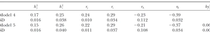
TABLE 4
Estimates of posterior means and standard deviations (SD), obtained from models 4 and 5, for heritability (h2), repeatability (r), environmental correlation (r
E), genetic correlation (rA), and proportion of variance due to herd-year-type of insemination effects (hy2)
h2
y h2z ry rz rA rE hy2y
Model 4 0.17 0.25 0.24 0.29 ⫺0.23 ⫺0.39
SD 0.016 0.038 0.010 0.034 0.112 0.032
Model 5 0.15 0.26 0.22 0.29 ⫺0.21 ⫺0.37 0.06
SD 0.016 0.040 0.011 0.037 0.108 0.034 0.007
Subscriptsyandzrefer to TNB and to WTAB, respectively.
Model assessment:Results from the model assessment discrepancy measures chosen is small. However, over
all the criteria explored, the HYT-Nor group of models study are shown in Table 6. Models 1 and 4 [those that
considered that herd-year-type of insemination effects performed better than the HYT-Un group of models.
Conditionally onz1, both groups of hierarchical
mod-were,a priori, uniformly distributed (HYT-Un) in Table
6] produced almost indistinguishable results. So did els tend to overpredict the difference between the
means of parity 2 records from selected and control models 2 and 5 [those that considered that
herd-year-type of insemination effects were,a priori, normally dis- lines (the observed difference is 0.40 piglets per litter),
with HYT-Nor behaving slightly better than HYT-Un. tributed (HYT-Nor)]. Therefore, to economize on the
presentation of results, these two sets of models were However, this observed difference is well within the
range of posterior uncertainty: the Monte Carlo esti-grouped. For TNB, the fact that there is no difference
in the behavior of single-trait and two-trait models con- mate of the 95% posterior interval of the marginal
poste-rior distribution of DSCunder HYT-Nor is (0.14, 1.12)
firms that WTAB does not contribute detectable
infor-mation to inferences about TNB. and under HYT-Un is (0.20, 1.15).
The estimates of marginal likelihoods provide very The first two rows of Table 6 compare the two groups
of hierarchical models. The difference between the nat- strong evidence against the NH model. This is consistent
with the observation that the posterior distribution of ural logarithms of marginal likelihood (the logarithm
of the Bayes factor) providesvery strongevidence (using heritability assigns most of the probability mass away
from zero. The NH model predicts the average observed
the standard in Kass and Raftery 1995) in favor of
models that assume herd-year-type of insemination ef- difference of parity 2 records between selected and
con-trol lines very accurately. However, the posterior
uncer-fects are,a priori, normally distributed, relative to the
alternative HYT-Un group of models. In fact, if equal tainty of this predictive distribution is much larger than
that obtained fitting the hierarchical models.
probabilities are assigned for the two models a priori,
the results obtained indicate that model HYT-Nor is All the models implemented in this study
underpre-dict extreme observations (last two columns of Table
exp(30.8) times more likelya posteriorithan model
HYT-Un. A similar conclusion favoring the HYT-Nor model 6). A closer look at the extreme observations did not
produce insight as the underlying cause for this result; based on a likelihood analysis, a different data set, and
a different criterion of model assessment was arrived at errors in recording cannot be dismissed. The NH model
performs worse than the hierarchical models; it per-byEstanyandSorensen(1995).
Despite the rather marked difference in the marginal forms poorly also, relative to the hierarchical models,
in predicting individual records, on average. likelihoods, the difference between the two groups of
models to predict specific features of the data via the A little digression is in place to describe the
computa-TABLE 5
Estimates of posterior means of response to selection for TNB at generations 1 (Rˆ1) and 2 (Rˆ2) and of posterior means of the correlated responses for WTAB (in grams) at generations 1 (CR
典
1)and 2 (CR
典
2), fitting Models 4 and 5TNB WTAB
Rˆ1 Rˆ2 CR
典
1 CR
典
2
Model 4 0.48(0.12) 0.60(0.14) ⫺8.4(13.8) ⫺17.4(15.6)
Model 5 0.43(0.10) 0.52(0.12) ⫺7.2(13.3) ⫺15.0(15.03)
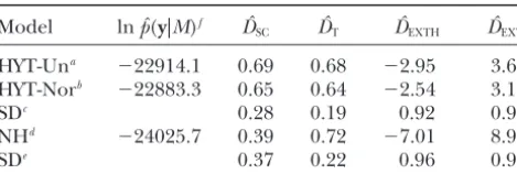
TABLE 6 tion of an estimator in conceptual repetitions of the experiment under identical conditions. Bayesian
meth-Model comparison via marginal likelihoods and
ods used in conjunction with MCMC provide
consider-discrepancy measures
able freedom in building hierarchical models that de-scribe the perceived underlying structures in the data.
Model lnpˆ(y|M)f Dˆ
SC DˆT DˆEXTH DˆEXTL
We have also illustrated how a Bayesian analysis used in
HYT-Una ⫺22914.1 0.69 0.68 ⫺2.95 3.61
conjunction with MCMC allows models to be compared
HYT-Norb ⫺22883.3 0.65 0.64 ⫺2.54 3.19
using a variety of criteria and how a sensitivity
analy-SDc 0.28 0.19 0.92 0.90
sis—to the prior distribution or to the likelihood—can
NHd ⫺24025.7 0.39 0.72 ⫺7.01 8.97
be implemented.
SDe 0.37 0.22 0.96 0.95
Concerning TNB, the most parsimonious model, the
Monte Carlo estimates of log marginal likelihood, lnpˆ(y|M)
NH model yielded an estimate of selection response of
(computed using Equation 15), and Monte Carlo estimates
0.40 piglets per litter. Point inferences using this simple
of posterior means of discrepancy measures (DˆSC, difference
between average of parity of two simulated records in selected model are appealing, because no assumptions are made
and control lines; the observed difference is 0.40 piglets per about the underlying genetic model (Sorensen and litter);DˆT, average difference between observed and simulated Kennedy1986). The mean of the posterior distribution data;DˆEXTH, average difference between highest extreme
ob-of selection response,E(R1|y), is approximately equal
served and simulated records; DˆEXTL, average difference
be-toy1...⫺y2..., the difference between phenotypic means
tween lowest extreme observed and simulated records.
aModels 1 and 4 (herd-year-type of insemination uniformly of the selected and control lines. Thus, using the NH
distributed,a priori). model response is evaluated using data from these lines
bModels 2 and 5 (herd-year-type of insemination normally
only.
distributed,a priori).
This is in contrast to the more highly parameterized
dNonhierarchical NH model, slightly modified for the
com-additive genetic models, which invoke an infinitesimal
putation ofpˆ(y|M)—see text for explanation.
c,eApproximate standard deviation of posterior distribution additive model as the genetic mechanism through
associated with the hierarchical/NH models. which response to selection is generated. These models
fEmpirical Monte Carlo standard error of lnpˆ(y|M): 6.2.
were fitted here using the Gibbs sampler. The properties of this approach to the analysis of selection experiments
are described inSorensenet al.(1994). Very succinctly,
tion of the marginal likelihood associated with the NH we mention here that, in general, the Bayesian approach
model. Expression (14) shows that the Bayes factor is provides a unified way of drawing inferences about
vari-undetermined whenp(i|Mi) is improper, as defined in ances and selection response, without recourse to
ana-the NH model. To circumvent this problem,pˆ(y|M⫽ lytic approximations or toad hocarguments. The
poste-NH), where M ⫽ NH refers to the NH model, was rior variance of a parameter in question (or a function
computed with a model similar to the NH model, except of it), obtained here empirically via the Gibbs sampler,
that [b] was assigned a uniform distribution with sup- provides a probabilistic description of uncertainty,
port defined by upper and lower limits bmin ⫽ 0 and which accounts for the loss of information incurred in
bmax ⫽ 20(0 and20are vectors of order equal to the the estimation of other parameters of the model.
number of elements inb). Further,2
e was assigned a Posterior variances account for genetic drift; in a
uniform prior with lower limit equal to 0 and upper Bayesian setting, genetic drift can be interpreted as the
limit equal to 20.0. Several other runs with varying limits relative loss of information about the genetic mean that
for [b] and [2
e] gave virtually identical results. evolves with time, due to the increased correlated
struc-Discrepancy measures derived from the predictive ture in the data that builds as the experiment progresses.
densityp(z2|z1,Mi) were computed using the unmodified As a result of this, say, when the number of additive
NH model, because p(z2|z1, Mi) is not affected by the genetic values contributing to the (additive) genetic
impropriety of prior distributions. In fact, it can be means of the different generations is the same, the
pos-shown thatp(z2|z1,Mi) has the form of a multivariate terior variance of the genetic mean increases with
gener-t-distribution. ations.
In the analyses based on hierarchical models, the whole data on which selection decisions were taken are
DISCUSSION
included in the analysis. This holds for the analysis of direct response to selection for TNB and for the analysis The majority of the analyses presented in this work
were based on the Bayesian approach to inference. An of correlated response for WTAB. Therefore, joint and
marginal posterior distributions are not affected by se-important objective of this work is to illustrate how this
approach allows the analyst to quantify probabilistically lection (Gianola and Fernando 1986). This implies
that it is not required to model the selection process to the uncertainty involved in the description of direct and
correlated selection responses. This is done condition- draw inferences.
Expressions of response to selection obtained via the ally on the data at hand, without invoking the use of
from the prior distribution, from what we have called ence (0.65vs. 0.40), the observed value of 0.40 piglets per litter is well within the range of posterior uncer-the base and from animals that belonged to uncer-the selected
and control lines in the common farm. The latter group tainty. We note also that the numbers in Table 6 show
that the variance of the posterior predictive difference comprised 1072 litter records, whereas the former
con-tributed 8988 litter records. An attempt was made to is 1.75 times larger in the case of the NH model.
Litter size is known to be affected by inbreeding de-quantify the information coming from these sources
using the concept of observed statistical information pression—a phenomenon that the additive genetic
models implemented in this study are unable to explain. and appealing to asymptotic results to estimate it. The
amount of information [as defined in (13)] contributed To account for inbreeding depression, some form of
interaction effects within or between loci, or both, is by the prior distribution and by the 8988 litter records,
relative to that from the selected and control lines, was required as part of the mechanism responsible for
ge-netic variation. Another way of testing the operational almost 70%, and this number was consistent for all the
prior distributions studied. In other words, had the lines adequacy of the additive genetic model is to compare
predictions of crossbred performance under such a not differed phenotypically in TNB, the additive genetic
model-based inferences would have yielded a positive model, using data from purebred performance.
Ander-sen et al. (1998) carried out such comparisons using response. This is why it is important, especially from a
genetic point of view, to contrast results obtained by purebred data from Danish Yorkshire and Landrace
and the crossbred data from both breeds. The results fitting the additive genetic models and the NH model,
which infers response to selection using the difference of their analysis were consistent with what one would
expect, assuming an additive genetic model. Under the between the means of selected and control lines only.
In our experiment, both types of models yielded similar low levels of inbreeding characteristic in the data from
these studies, the added computational burden involved inferences about selection response. This agreement is
indicative that an additive genetic model is operationally to account for nonadditive gene action does not seem
to be justified. adequate to describe the results of this experiment.
Once this point is confirmed, there is little doubt that The analysis of TNB and WTAB with model 5
indi-cates that the posterior probability that the correlated the hierarchical model yields a much sharper picture
of the outcome of the selection experiment. The Monte response in WTAB is negative isⵑ76%. The 95%
poste-rior probability interval for the genetic correlation is Carlo estimate of the 95% probability interval of
selec-tion response for TNB based on the hierarchical model (⫺0.46; ⫺0.01), and the Monte Carlo estimate of the
mean of the posterior distribution is⫺0.21. The
conclu-HYT-Nor is (0.23, 0.60); the corresponding interval
from the NH model is (⫺0.07, 0.89). sions based on these numbers are qualitatively in
agree-ment with those of Kerr and Cameron (1995) and
The model assessment study shows that the most
ap-propriate model among the ones fitted was the hierar- Roehe(1999).Roehe(1999) used TNB as a covariate
in a model for individual birth weights and he found chical model, which assumes that herd-year-type of
in-semination effects are, a priori, normally distributed. that these decrease by 44 g with each additional piglet
born.KerrandCameron(1995) found that individual
This conclusion is based on the marginal likelihood,
which is a global test of the model, and on the ability birth weight decreases by 30 g with each additional
piglet born. On the basis of the numbers in Table 4, a of the models to predict specific features of the data.
Due to the present experimental protocol, it was judged genetic regression of 55 g per born piglet is obtained,
and a phenotypic regression of 23 g per born piglet. meaningful to study the latter, generating simulated
data from posterior predictive distributions under a vari- Litter size has been part of the Danish breeding
objec-tive since 1992. The decision is fully justified on the ety of models, conditional on data from base individuals.
Replicated data could have easily been simulated from grounds of the results of this experiment. However, it
seems prudent to monitor birth weight and piglet viabil-posterior predictive distributions under the various
models, rather than conditioning on the base records. ity, together with other components of reproduction,
to avoid undesirable genetic changes. The general idea here is to study the ability of the
models to generate replicated data that look similar to
the data actually observed (Gelman et al.1995).
Among the criteria used to compare models, the NH LITERATURE CITED
model performed worse than the hierarchical models Andersen, S., B. PedersenandA. Vernersen,1998 Impact of
nu-cleus selection at production level. Proceedings of the 6th World
in all cases, except in the ability to predict the difference
Congress on Genetics Applied to Livestock Production, Armidale,
between the raw means of selected and control lines
Australia. Vol. XXIII, pp. 515–518.
among parity 2 records. This statement is based on the A´ valos, E.,andC. Smith,1987 Genetic improvement of litter size
in pigs. Anim. Prod.44:153–164.
mean of the relevant posterior distribution as a criterion
Bichard, M.,andC. M. Seidel,1983 Selection for reproductive
to decide what is “best.” However, despite the fact that
performance in maternal lines of pigs. Proceedings of the 2nd
the hierarchical models yield a mean of the posterior World Congress on Genetics Applied to Livestock Production,
Madrid, Spain. Vol. VIII, pp. 565–569.