Genotypic variation for a quantitative character maintained under stabilizing selection without mutations: epistasis.

(1)

Genotypic Variation for a Quantitative Character Maintained Under

Stabilizing Selection Without Mutations: Epistasis

A. Gimelfarb

Department of Ecology and Evolution, The University of Chicago, Chicago, Illinois 60637 Manuscript received March 30, 1989

Accepted for publication June 2, 1989

ABSTRACT

A model of the gene action on a quantitative character is suggested. The model takes into account epistasis by combining multiplicative with the traditional additive approximation of the action of loci. It is demonstrated on the basis of this model that a high level of genotypic variation can be maintained in a population for a quantitative character under stabilizing selection in the absence of mutations, if

there is epistasis. It is also shown that a large amount of additive variation as well as high heritability

can be “hidden” in such a population and “released if stabilizing selection is relaxed.

S

TABILIZING selection for an intermediate phenotype is widely recognized as a very important factor acting on quantitative characters in natural populations. It is also widely recognized that the presence of genotypic variation, and additive genotypic variation in particular, for a quantitative character is necessary for its evolution. On the other hand, starting from

R.

A. FISHER (1930), it has been demonstrated that the effect of stabilizing selection on a character is to reduce its additive component of genotypic variance. LEWONTIN (1964) has shown that no genotypic variation at all (except for variation due to one seg- regating locus) can be maintained under stabilizing selection for a quantitative character controlled by a genetic system with several equivalent loci, if the effect of genes on the character is strictly additive. A similar result was obtained by BULMER (197 1). And yet many field and laboratory studies often reveal substantial amounts of genotypic variation maintained by quantitative characters in natural populations. Also, the fact that many quantitative characters show an appreciable response to artificial selection indicates that a large proportion of the maintained genotypic variation is additive. To account for this, a hypothesis of “mutation-selection balance” as a mechanism responsible for maintenance of genotypic variation in natural populations was put forward and several models of such a mechanism have been suggested [SLATKIN (1987) can be consulted for references]. T h e idea of variation maintained by mutation-selection balance is in itself quite obvious. Indeed, given that selection reduces variation whereas mutations increase it, there is going to be some variation maintained due to a balance between the two forces. It is not quite as

T h e publication costs of this article were partly defrayed by the payment of page charges. This article must therefore be hereby marked “advertisement”

in accordance with 18 U.S.C. $1734 solely to indicate this fact. Genetics 123: 217-227 (September, 1989)

obvious, however, whether parameters of selection and mutations in nature are such that this mechanism can actually account for the high levels of genetic variation often observed in natural populations.

Selection and mutations are not the only factors affecting variation in a population. Various other processes of hereditary transmission (segregation, recombination, etc.) also have an effect. If these processes are such that individuals of intermediate phenotypes produce a sufficient number of offspring with extreme phenotypes, then, even in the absence of mutations, there will be two forces having opposite effects on variation: stabilizing selection reducing it and hereditary transmission increasing it. A balance between these forces may result in maintenance of genotypic variation.

(2)

218 A. Gimelfarb

transmission is the model by GALE and KEARSEY

(1 968) (also KEARSEY and GALE 1968) of quantitative characters controlled by two or three loci without dominance but with non-equal effects on the character. A stable polymorphic equilibrium under stabilizing selection for an intermediate phenotype is possible in this model, but this requires large differences between the effects of the loci. It appears, therefore, that this mechanism also cannot account for the variation maintained for characters controlled by many loci.

All existing models of mutation-selection balance (and practically all population genetic models of quantitative characters) assume additivity of the action of loci and ignore epistasis. Very few arguments have been offered, however, to justify this. One of the main arguments comes from the fact that little epistasis is usually detected when methods of statistical analysis based on partitioning the total phenotypic variance are employed. It is important, however, to recognize the difference between epistasis as a nonadditive action of loci controlling a character and “epistasis” measured by the component of the total genotypic variance attributable to the nonadditive action of the loci. T h e “epistatic component of variance” depends on a particular distribution of genotypes, and, hence, “epistasis” measured by such a component does not represent a property of a quantitative character, but rather a characteristic of a particular population. Therefore, the fact that very little variation is attributable to non-additivity in the action of loci does not necessarily mean that the loci do indeed act additively.

ADDITIVE-MULTIPLICATIVE MODEL OF LOCUS

ACTION

One of the problems in dealing with epistasis is the difficulty of incorporating it into a manageable model. Quite a few parameters are needed to represent general epistasis even in the case of only two loci, and the number of parameters grows very rapidly when the number of loci increases. T h e purpose of this paper, however, is not to suggest a general model of epistasis, but rather to demonstrate that it can be responsible for the maintenance of high levels of genotypic variation in populations under stabilizing selection. We shall also limit our consideration only to “pure” epistasis, i.e., dominance and unequal effects of loci will not be considered.

Consider two diallelic loci, A and B . Since dominance is excluded and the loci are assumed to be equivalent, only one parameter is needed (ignoring a linear scale transformation) to describe any epistasis in this case, and the following matrix may be used to

represent the genotypic values corresponding to different genotypes:

A a 1-2 2 - 2 3-2

aa 2-22 3 - 2

4

Defining the effects, XA and xB, of

genotypic value:

Locus Effect

Genotype xA, XB

AA, BB 0

A a , Bb 1 a a , bb 2

BB Bb 66

AA 0 1-2 2 - 2 2

(1)

the loci on the

( 2 )

it is not difficult to verify from (1) that the genotypic value, x, of an individual with a particular genotype can be represented as

x = (1

-

%)(xA

+

x B )

+

%(xAxB). ( 3 4

Thus, a “pure” (additive by additive) epistatic interaction between two diallelic loci can always be represented as a sum of two components: additive and multiplicative.

T h e “additive-multiplicative” model of epistasis can be extended to more than two loci, so that the genotypic values for three and four loci are represented as:

X = (1

-

z)(xA

+

XB

+

xC)

+

z(xAxBxC), (3b)

X = (1

-

z)(xA

+

XB

+

xc

+

x g )

+

z(xAxBxCXD), ( 3 ~ )

with the effects of loci C and D being the same as those of loci A and B in (2). Limiting our consideration to 0 5 z 5 1, parameter z of the model can be interpreted as the “strength” of epistasis. When z = 0 , the effects of loci are strictly additive and there is no epitasis, whereas z = 1 means a purely multiplicative interaction between the loci. T h e range of genotypic values is between xmin = 0 and x,,, = (1

-

2 ) 2 n

+

z2“,

where n is the number of loci.

(3)

a combination of two scales widely used in practical applications: linear and logarithmic. Indeed, if a logarithmic transformation makes a character “more additive,’’ this implies that on the original, linear scale the effects of the loci were multiplicative. POWERS (1950) presents specific examples of the use of linear and logarithmic scales.

Stabilizing selection on the genotypic values of a quantitative character can be described by a quadratic function representing the fitness of an individual with the genotypic value x:

w ( x ) = 1

-

K ( x - e?)? (4)

T h e “optimum” genotypic value, 8, was fixed in all cases exactly in the middle of the range of genotypic values (although this is not critical for the results):

0 = ‘12 (X,,,

-

Xmin), ( 5 )

where xn,in and xmaX are the minimum and maximum genotypic values for a given strength of epistasis, z. T o ensure that the fitness function remains nonnega- tive for any x within the range of genotypic values, the fitness function was represented in the following form:

where S takes values between 0 and 1 and can be regarded as the strength of selection (the greater S is, the stronger selection is). An individual with the optimal genotypic value, 19, always has the maximum fitness, 1, whereas individuals with extreme genotypic values, 0 and x,,,, have the lowest fitness, 1

-

S.

T h e effect of environment on a quantitative character was neglected, but it can be easily accommodated by ap- propriately correcting parameters of the fitness function (6).

Considering a two-locus case, it is seen from (1) that the fitnesses of genotypes are described by a matrix of the following type:

BB Bb bb

A A a b c

A a b d e

(7)

a a c e a

which is a special case of a two-locus model discussed by FRANKLIN and FELDDAN (1 977). Although matrix

(7)

is symmetric, the model is not the “symmetric viability model” (in which case b = e ) discussed by BODMER and FELSENSTEIN (1 967) and also by KARLIN and FELDMAN (1970). For the latter model there always exists an equilibrium with

p,

=

pB

= 0.5 for any recombination and actual values of fitnesses. Equilib- ria in model (7), instead, depend on the recombination as well as on the actual values of fitnesses and it is quite difficult to find such an equilibrium analytically.

It is even more difficult to find equilibria and investi- gate their stability analytically when the number of loci is greater than two. For this reason, computer modeling was employed. All computations were conducted on a microcomputer “Compaq 11.”

COMPUTER MODELING

Random mating was assumed, and the following system of recurrence equations was used to describe the dynamics of the gametic distribution in a population:

qk+l(g3)

wk

= qk(gl)qk(g2)W(gl, g2). g l g 2

Here, g l , g 2 and g3 are gametes (e.g., Ab in the case of two loci, aBC in the case of three loci or AbcD in the case of four loci); q k and qk+l are the proportions of gametes in generations k and k

+

1. T h e fitness, w , of a genotype ( g l , gz), is obtained by computing for this genotype the genotypic value based on formulas

(2)

and (3) and substituting it into the formula for the fitness function (6). Function H(g3 Igl, g2) in (8) represents the conditional probability that a gamete pro- duced by an individual with the genotype ( g l , g2) will be gs. A program for computing this function can be written for any set of recombination coefficients.

Given the gametic frequencies in a particular generation, it is not difficult to compute allelic frequencies and linkage disequilibria. It is also not difficult to obtain, assuming random mating, the distribution of genotypic values, and, hence, the mean and the variance of the genotypic values in a given generation.

Let us assume that the coefficients of recombination between two adjacent loci are the same for all loci and that there is no interference. Combined with the assumption of equivalent loci this entails a symmetry in the model, so that conditions

P A = P E (for two loci)

P A = P C (for three loci) (9)

P A = P D , P B = P C : (for four loci)

(where P A , P B ,

PC

and

p,

denote the allelic frequencies

in corresponding loci) are invariant with respect to the dynamic equations (8). Only symmetric equilibria of type (9) have been studied in this paper. It should be pointed out that nonsymmetric equilibria may also exist even for a symmetric model (KARLIN and FELD-

Equilibria were obtained by numerically iterating recurrence equations (8). T h e “distance,” d , between the distributions of gametes in two consecutive generations,

(4)

220 A. Girnelfarb

d =

Jc

[ Q k + l k )

-

Q k ( g ) I 2 , (10)

g

was computed after every iteration, and when d

<

1 O”’, it was determined that an equilibrium has been

reached. Since only symmetric equilibria were considered, in order to speed up the computations, iterations were always started with allelic frequencies being 0.5

in all loci, i.e., conditions (9) were satisfied from the beginning. Also, gametes initially were in linkage equilibrium.

After an equilibrium solution of (8) has been obtained, a test of its stability was performed. In the case of two loci, the system of equations (8) was linearized at the equilibrium yielding a cubic characteristic equation. T h e roots of this equation were computed, and the stability of the equilibrium was determined based on the eigenvalues. Thus, a standard local stability analysis was performed in the case of two loci. T h e characteristic equations for three and four loci are too complex, and the stability of equilibria in those cases was tested in a different way. After obtaining an equilibrium in those cases, the equilibrium distribution of gametes was perturbed by adding to each gametic frequency its own independently generated random number uniformly distributed between 0 and 0.1, and then normalizing the gametic frequencies to unity. The system (8) was then iterated again starting with the randomly perturbed gametic frequencies. At least two random perturbations of an equilibrium were performed. If after each perturbation the system converged back to the previously established equilibrium, it was classified as stable, and it was classified as unstable otherwise. T h e justification for such a method of determining local stability of an equilibrium is presented in APPENDIX

c.

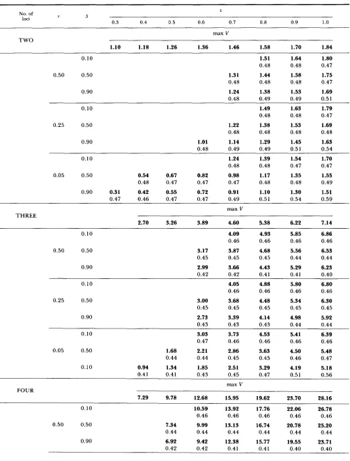
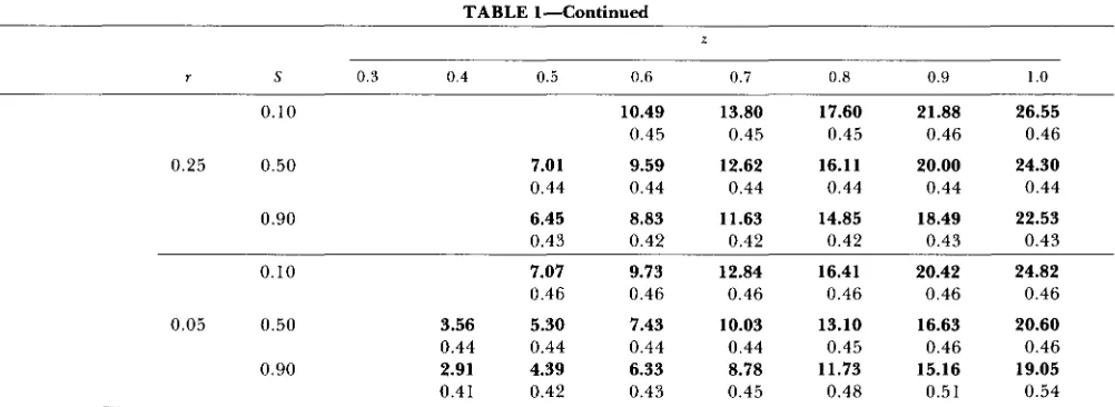
T h e main results of computer modeling are sum- marized in Tables 1 and 2. It should be pointed out that only stable equilibria with all loci being polymorphic with allelic frequencies above 0.1 are included in the tables. Blank spaces in a table indicate the lack of such a “totally polymorphic” stable equilibrium. It is also worth noting that there was negative linkage disequilibrium between each pair of loci in all stable equilibria.

T h e genotypic variances maintained in stable equilibria are presented in Table 1. A bold entry shows the genotypic variance, V, maintained by a character with the strength of epistasis z and recombination coefficient r under selection of strength S . T h e value of V in itself does not tell whether the level of maintained variation is high or low. An answer to this question can be obtained by comparing the value of V maintained under selection with the maximum genotypic variance that can ever be maintained for the character under random mating without any selection. The values of the maximum genotypic variance, max V, for a corresponding strength of epistasis z are

also included in Table 1. T h e analytical derivation of the maximum variance for two loci is given in APPEN- DIX A. For three and four loci analytical derivations are too complex and the following computer procedure was employed instead. Genotypic variances were computed for a given value of z under the assumption of linkage equilibrium for a grid of allelic frequencies between 0 and 1 with a step 0.005, and the highest among them was chosen as the maximum.

Also included in Table 1 (regular numbers) are the coefficients of linear offspring-parent regression, 6, in a population at a stable equilibrium. They were computed according to the formulas presented in APPEN-

DIX D. This coefficient is often used to estimate the heritability ( h 2 = 26). Notice that with epistasis the values of this coefficient may exceed 0.5 resulting in nonsensical estimates of the heritability. This is due to the fact that 6 represents the coefficient of the linear regression best fitted to the actual offspring- parent regression which may be nonlinear in the presence of epistasis.

How much of the equilibrium genotypic variance is additive? Before answering this question, recall that there is a negative linkage disequilibrium in all stable equilibria in Table 1. A partitioning of the genotypic variance into additive and epistatic components is not very useful in the presence of linkage disequilibrium. This is because the separation of main effects and interactions in a factorial design is meaningful only if the factors are independent, whereas their meaning is much less obvious when the factors are not independent. APPENDIX B provides an illustration of a situation when notions of additive variance and heritability are useless for predicting responses to selection in the presence of linkage disequilibrium. BULMER (1985, pp. 160-1 63) and GRIFFINC (1960) also discuss this problem.

We may, however, compute the additive variance and heritability for a population with the same allelic frequencies as those maintained under stabilizing selection, but in linkage equilibrium. Computed in this manner, additive variance and heritability can be regarded as “hidden” in the population at the equilibrium under stabilizing selection, and “released” when selection is relaxed. It is as if a sample from a population in nature (where natural selection operates) is brought to a laboratory (where it is relaxed) and individuals are allowed to mate randomly for a number of generations before estimates of additive variance and heritability are undertaken. This may be close to what quite often happens in reality.

(5)

TABLE 1

Genotypic variance (bold numbers) and offspring-parent regression (regular numbers) maintained in a stable equilibrium under stabilizing selection

z No. of

loci r S

0.3 0.4 0.5 0.6 0.7 0.8 0.9 1 .o

max V TWO

1.10 1.18 1.26 1.36 1.46 1.58 1.70 1.84

0.10

0.50 0.50

0.90

1.51 1.64 1.80

0.48 0.48 0.47

1.31 1.44 1.58 1.75

0.48 0.48 0.48 0.47

1.24 1.38 1.53 1.69

0.48 0.49 0.49 0.51

0.10

0.25 0.50

1.49 1.63 1.79

0.48 0.48 0.47

1.22 1.38 1.53 1.69

0.48 0.48 0.48 0.48

0.90 1.01 1.14 1.29 1.45 1.63

0.48 0.49 0.49 0.51 0.54

0.10 1.24 1.39 1.54 1.70

0.48 0.48 0.47 0.47

0.05 0.50 0.54 0.67 0.82 0.98 1.17 1.35 1.55

0.48 0.47 0.47 0.47 0.48 0.48 0.49

0.90 0.31 0.42 0.55 0.72 0.91 1.10 1.30 1.51

0.47 0.46 0.47 0.47 0.49 0.51 0.54 0.59

max V THREE

2.70 3.26 3.89 4.60 5.38 6.22 7.14

0.10

0.50 0.50

0.90

4.09 4.93 5.85 6.86

0.46 0.46 0.46 0.46

3.17 3.87 4.68 5.56 6.53

0.45 0.45 0.45 0.44 0.44

2.99 3.66 4.43 5.29 6.23

0.42 0.42 0.41 0.41 0.40

0.10

0.25 0.50

4.05 4.88 5.80 6.80

0.46 0.46 0.46 0.46

3.00 3.68 4.48 5.34 6.30

0.45 0.45 0.45 0.45 0.45

0.90 2.73 3.39 4.14 4.98 5.92

0.43 0.43 0.43 0.44 0.44

0.10 3.03 3.73 4.53 5.41 6.39

0.47 0.46 0.46 0.46 0.46

0.05 0.50 1.68 2.21 2.86 3.63 4.50 5.48

0.44 0.44 0.45 0.45 0.46 0.47

0.10 0.94 1.34 1.85 2.51 3.29 4.19 5.18

0.4 1 0.41 0.43 0.45 0.47 0.5 1 0.56

max V FOUR

7.29 9.78 12.68 15.95 19.62 23.70 28.16

0.10

0.50 0.50

0.90

~ 10.59 13.92 17.76 22.06 26.78

0.46 0.46 0.46 0.46 0.46

~~

7.34 9.99 13.13 16.74 20.78 25.20

0.44 0.44 0.44 0.44 0.44 0.44

6.92 9.42 12.38 15.77 19.55 23.71

(6)

2 2 2 A. Gimelfarb

TABLE 1-Continued

z

r S 0.3 0.4 0.5 0.6 0.7 0.8 0.9 1 .O

0.10 10.49 13.80 17.60 21.88 26.55

0.45 0.45 0.45 0.46 0.46

0.25 0.50 9.59 7.01 12.62 16.11 20.00 24.30

0.44 0.44 0.44 0.44 0.44 0.44

0.90 8.83 6.45 11.63 14.85 18.49 22.53

0.43 0.42 0.42 0.42 0.43 0.43

0.10 9.73 7.07 12.84 16.41 20.42 24.82

0.46 0.46 0.46 0.46 0.46 0.46

0.05 0.50 3.56 7.43 5.30 10.03 13.10 16.63 20.60

0.44 0.44 0.44 0.44 0.45 0.46 0.46

0.90 2.91 6.33 4.39 8.78 11.73 15.16 19.05

0.41 0.42 0.43 0.45 0.48 0.51 0.54

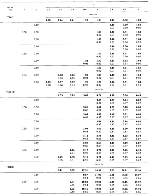
z = parameter of epistasis; 7 = recombination; S = strength of selection; max V = maximum genotypic variance without selection. additive genotypic variance were conducted following

CROW and KUMURA (1970). T h e derivation of the

maximum additive variance for two loci is given in the APPENDIX A , whereas for three and four loci it was computed using a grid procedure similar to the one used to obtain the maximum genotypic variance in Table 1. T h e “hidden” heritability in Table 2 is de- fined as the ratio of the “hidden” additive variance to V*, the total genotypic variance computed with allelic frequencies determined by stabilizing selection, but in linkage equilibrium. Due to the negative linkage equilibrium, V*

>

V.

DISCUSSION AND CONCLUSIONS

Results in Table 1 clearly demonstrate that large amounts of genotypic variation (close to the maximum possible without selection) can be maintained for a quantitative character with epistasis under stabilizing selection in the absence of mutations. This may hap- pen under weak ( S = 0.1) as well as under strong ( S = 0.9) selection. It may also be pointed out that the equilibrium mean genotypic value, although not being exactly equal to the “optimum,” is not very far from it: the ratio of the equilibrium mean, M , to the “optimum” value, 8, was in all cases within the interval 0.82

I M/B I 0.95, 0.83 I M/B 5 0.92 and 0.86 I M/B 5

0.9 1 for two, three and four loci, respectively. Notice also that, unlike the genotypic variance maintained

d u e to dominance which goes down when the number

of loci increases (LEWONTIN 1964), the variance maintained due to multiplicative epistasis grows almost geometrically with increasing number of loci.

It is not only that a large amount of genotypic variation can be maintained for a quantitative character with epistasis in a population under stabilizing selection, but, as results in Table

2

demonstrate, a large amount of additive variation can be “hidden” in such a population. Table 2 also shows that the corresponding “hidden” heritabilities can be quite high

(greater than 0.8 in all cases). This means that almost all genotypic variation “released” from the equilibrium population by relaxing the stabilizing selection will be additive, and, hence, methods based on esti- mating the epistatic component of variance will practically never detect even a strong multiplicative interaction between loci. It also means that there will be an appreciable linear response to directional selection in such a population, ie., the character controlled

by

epistatic loci will respond as if the action of the loci was almost purely additive.

Thus, an important conclusion from Tables 1 and

2

is that, on one hand, a large amount of genotypic variation can be maintained under stabilizing selection by a character with epistasis, but on the other hand, such epistasis may never be detected by either a standard genetic-statistical technique or by the response of the character to directional selection.

(7)

TABLE 2

“Hidden” additive variance (bold numbers) and heritability (regular numbers) maintained under stabilizing selection

z

No. of

loci r S 0.3 0.4 0.5 0.6 0.7 0.8 0.9 1 .o

max Va TWO

1.08 1.14 1.21 1.29 1.38 1.48 1.58 1.69

0.10 1.40 1.50 1.63

0.91 0.90 0.90

0.50 0.50

0.90

1.30 1.40 1.51 1.63

0.92 0.91 0.90 0.90

1.30 1.40 1.51 1.64

0.92 0.91 0.90 0.90

0.10

0.25 0.50

1.40 1.50 1.63

0.91 0.90 0.90

1.30 1.40 1.51 1.64

0.92 0.91 0.90 0.90

0.90 1.22 1.30 1.41 1.52 1.64

0.94 0.92 0.91 0.91 0.90

0.10 1.30 1.40 1.51 1.63

0.92 0.91 0.9 1 0.90

0.05 0.50 1.08 1.13 1.20 1.29 1.40 1.51 1.64

0.96 0.95 0.94 0.92 0.91 0.91 0.90

0.90 1.03 1.07 1.12 1.20 1.29 1.40 1.51 1.64

0.98 0.96 0.94 0.93 0.92 0.91 0.9 1 0.90

T H R E E

max Va

2.55 3.04 3.60 4.22 4.90 5.64 6.43

0.10 3.63 4.33 5.14 6.02

0.87 0.87 0.87 0.87

0.50 0.50

0.90

3.06 3.67 4.37 5.18 6.06

0.88 0.87 0.87 0.87 0.87

3.09 3.69 4.40 5.21 6.08

0.88 0.87 0.87 0.87 0.87

0.10

0.25 0.50

3.64 4.34 5.14 6.03

0.87 0.87 0.87 0.87

3.09 3.69 4.40 5.20 6.08

0.88 0.87 0.87 0.87 0.87

0.90 3.12 3.73 4.43 5.23 6.10

0.88 0.88 0.87 0.87 0.87

0.10 3.08 3.69 4.40 5.19 6.07

0.89 0.88 0.87 0.87 0.87

0.05 0.50 2.65 3.17 3.77 4.46 5.25 6.10

0.91 0.90 0.88 0.87 0.87 0.87

0.90 2.23 2.68 3.18 3.77 4.46 5.25 6.10

0.93 0.91 0.90 0.88 0.87 0.87 0.87

max Vu

6.71 8.93 12.51 14.39 17.63 21.21 25.10 FOUR

0.10 9.87 11.90 15.21 18.98 23.17

0.84 0.84 0.84 0.85 0.85

0.50 0.50 6.84 10.03 12.07 15.39 19.15 23.32

0.85 0.84 0.84 0.85 0.85 0.85

0.90 6.93 10.16 12.22 15.53 19.28 23.39

(8)

224 A . Gimelfarb

TABLE 2-Continued

2

r S 0.3 0.4 0.5 0.6 0.7 0.8 0.9 1 .o

0.10 9.90

0.84

11.93

0.84

15.25

0.84

19.03

0.85

23.19

0.85

0.25 0.50 6.91 10.13

0.85

12.17

0.85

15.50

0.85 0.85 19.26 0.85 23.39 0.86

0.90 7.05 10.31 12.35 19.39 23.47

0.86 0.85 0.85 0.85 0.85 0.86

0.10 6.87 9.28 12.15

0.86

15.47

0.85

19.22

0.85

23.37

0.85 0.85 0.86 0.05 0.50 5.25 7.30 9.72 12.56

0.88 0.86 0.85 0.85 15.82 19.48 0.85 0.86 23.53 0.86 0.90 5.47 7.45 9.83 12.64

0.88

15.86

0.86 0.86

19.49 23.51

0.85 0.85 0.86 0.86

15.66

z = parameter of epistasis; r = recombination; S = strength of selection; max Va = maximum additive variance without selection.

f i t n e s s

I 1 I 1 1 1 1 1 1 1 1 1 1 1 1 1

-8 -6 -4 -2 0 2 4 6 8 10 12 14 16 18 20 22 24

phenotypic (genotypic) value

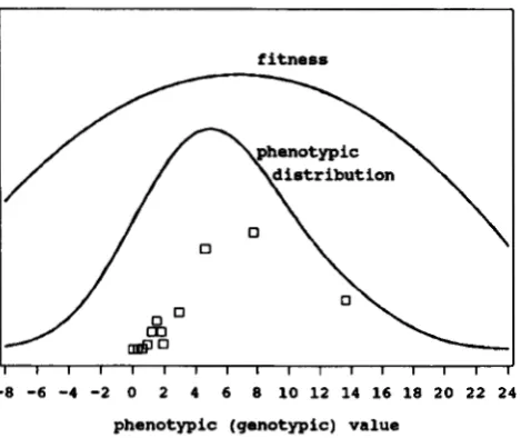
FIGURE 1 .-Equilibrium distribution under stabilizing selection of a quantitative character controlled by four epistatic loci and environment (the broad sense heritability, H z = 50%). T h e strength of epistasis, z = 0.7; the strength of genotypic selection, S = 0.1; recombination, r = 0.5. T h e scattered plot represents the frequencies of genotypic values.

zero mean and the variance equal to the genotypic variance, i e . , V , = V. T h e latter means that the broad sense heritability is 50%, which is close to values frequently observed in natural populations. T h e fitness of a phenotype X is described in this case by the following function (curve “fitness” in Figure 1):

W(X) = 1

-

O.O021(X

-

6.8)*, (1 1)

corresponding to the genotypic fitness function as in (6) with S = 0.1 (see GIMELFARB (1 984) for a discussion of the relationship between phenotypic and genotypic selection). Hardly anyone will find anything exotic about the phenotypic distribution in Figure 1. Hence, even strong epistasis may not manifest itself by an unusual phenotypic distribution.

A number of predictions can be made based on the additive-multiplicative model concerning the effect of the strength of stabilizing selection on the maintained genotypic variation as well as on the additive variance

and heritability. T h e genotypic variance (Table 1) maintained under stronger selection is reduced as compared to the gariance maintained under weaker selection, but the reduction is not necessarily very big, especially if the linkage is not tight. For example, when selection changes from S = 0.1 (weak) to S =

0.9 (strong), the equilibrium genotypic variance maintained by the genetic system with r = 0.5 and z = 0.7 is reduced from 4.09 to 3.66 for three loci, and from

13.92 to 12.38 for four loci (1 1 % decrease in both cases). This is not a big reduction considering how much stronger selection with S = 0.9 is as compared to one with S = 0.1. Indeed, the ratio of the fitness of the “optimal” genotype to that of the “worst” one is 10 when S = 0.9, whereas it is only 1.1 when S = 0.1. It is also seen from Table 1 that the coefficient of offspring-parent regression is practically unaffected either by the strength of selection or by recombination. As for the “hidden” additive variance (Table 2), it may actually increase, however slightly, when selection becomes stronger. T h e strength of selection has practically no effect on the “hidden” heritability (Table 2).

T h e above predictions of the additive-multiplicative model can be compared to the results of the few stabilizing selection experiments reported in the literature. FALCONER (1 957) conducted an experiment on the number of abdominal bristles on Drosophila melanogaster in which 20 out of 60 pairs of flies with the number of bristles nearest to the mean in the original population were selected for the duration of 14 generations. N o changes in the phenotypic variance that could be attributed to the selection were found, in spite of the relatively strong selection. In an

experiment by KAUFMAN, ENFIELD and COMSTOCK

(9)

TABLE 3

Three-locus genetic system with dominance and unequal effects of loci

Locus A Locus B Locus c

Genotype Effect Genotype Effect Genotype Effect

AA 0.00 BB 0.00 cc 0.00

Aa 0.80 Bb 1

.oo

cc

1.40

a a 2.00 bb 2.00 cc 2.40

lected (this procedure does not exactly correspond to the model of mass stabilizing selection considered in the present paper). There was a statistically significant decrease in the phenotypic variance under selection as compared to the control, but the reduction was not very large (15%) even after 95 generations. There was no significant change in the estimated additive variance, and only a very slight change in the heritability. T h e authors of both experiments offer a number of explanations for their results without invoking epistasis. However, as the additive-multiplicative model demonstrates, epistasis may also be an expla- nation.

Another interesting prediction of the additive-multiplicative model is that the “hidden” additive genotypic variation can increase with stronger epistasis (Table 2). For example, in the case of four loci with T

= 0.25 and S = 0.5, the amount of “hidden” additive variation is 6.91 when z = 0.5 (weaker epistasis) and 23.39 when z = 1.0 (strong epistasis). T h e ratio of the “hidden” additive variation to the maximum possible under linkage equilibrium is also lower when

z

= 0.5 than when z = 1 .O (0.77 us. 0.93). This indicates once again that the additive (or epistatic) component of genotypic variance may not be a good measure of the strength of epistasis.

T h e main conclusions of this paper are not limited to the sets of parameters actually used in computations and by the constraints imposed on the model to facil- itate the computations. T h e symmetry constraints (9) due to the assumption of no dominance, equivalent loci and equal recombination coefficients are not critical for the existence of a stable “total polymorphism.” For example, a three-locus model with the effects of loci being not as in (2) but as in Table 3 incorporates dominance and unequal effects of loci. With the strictly multiplicative interaction of loci

(z

= 1) and with the recombination coefficients TAB = 0.1 and rBC = 0.25, such a genetic system, although quite asym- metric, maintains under stabilizing selection (4) with S = 0.5 a stable equilibrium with all three loci being polymorphic: P A = 0.187, P B = 0.208, P C = 0.238.

Only selection with the “optimum” being exactly in the middle of the range of genotypic values was discussed in this paper. It is worth noting that neither dominance (LEWONTIN 1964) nor unequal effects of

loci (GALE and KEARSEY 1968; KEARSEY and GALE 1968) are capable of maintaining stable polymorphism with such an optimum. Computations show that the exact position of the optimum is not critical for the maintenance of a stable polymorphism by the additive- multiplicative model. For example, in the case of purely multiplicative interaction between three loci, when Xmin = 0 and X,,, = 8, a polymorphism can be maintained for a range of optima between 1.2 and 5.8. Moreover, shifting the optimum from being exactly in the middle may result in additional stable polymorphisms. Consider, for example, a character controlled by three loci with

z

= 0.5 and T = 0.5

under stabilizing selection of strength S = 0.9. T h e range of genotypic values for such a character is between 0 and 7.0. If 0 = 3.5, i.e., the optimum is exactly in the middle of the range of the genotypic values, there is no stable equilibria with all three loci being polymorphic (Table 1). If, however, 19 is shifted to 4.5, there is a stable equilibrium with allelic frequencies greater than 0.12 in all of the loci.

Many conclusions about quantitative characters reported in the literature are based on the additive approximation of gene action which ignores epistasis. T h e additive-multiplicative model discussed in this paper represents an extension of the additive model incorporating epistasis. This extension, being a step away from the traditional model, leads to new and important conclusions: mutations may not be needed in order for a high level of genotypic variation to be maintained in a population under stabilizing selection on a quantitative character and in order for a large amount of additive variation to be “hidden” in such a population. Mutations are, of course, indispensable as the main source of new heritable variation, and there is always going to be some genotypic variation maintained due to a balance between stabilizing selection and mutations. However, “mutation-selection balance” may not be the main mechanism responsible for the maintenance of heritable variation in natural populations.

I am very grateful to B. CHARLESWORTH, J. CROW, R. LANDE, T. NAGYLAKI, A. ORR, S. ORZACK, M. ROSE and M. WADE for their criticism and important suggestions. This work was supported in part by U.S. Public Health Service grant GM27120 (United States) and by a grant from Consiglio Nazionale delle Ricerche (Italy). I wish to express my gratitude to E. BOTTINI for his help.

LITERATURE CITED

BODMER, W. F., and J. FELSENSTEIN, 1967 Linkage and selection: theoretical analysis of the deterministic model. Genetics 57:

BULMER, M. G . , 1971 The stability of equilibria under selection.

BULMER, M. G., 1985 The Mathematical Theory of Quantitative

CROW, J. F., and M. KIMURA, 1970 An Introduction to Population

237-265.

Heredity 27: 157-162.

(10)

226 A. Gimelfarb

Genetics Theory. Harper & Row, New York.

FALCONER, D. S., 1957 Selection for phenotypic intermediates in

Drosophila. J. Genet. 55: 551-561.

FALCONER, D. S., 1960 Introduction to Quantitative Genetics. Ro- land Press, New York.

FISHER, R. A., 1930 The Genetical Theory of Natural Selection, Ed. 2. Longman, London.

FRANKLIN, I . R., and M. W. FELDMAN, 1977 Two loci with two alleles: linkage equilibrium and linkage disequilibrium can be simultaneously stable. Theor. Popul. Biol. 12: 95-1 13. GALE, j. S., and M. J. KEARSEY, 1968 Stable equilibria in the

absence of dominance. Heredity 23: 553-561.

GIMELFARB, A , , 1984 The significance of specific distributions and functions in models of quantitative inheritance. J. Math. Biol. 21: 205-2 1 1.

GRIFFING, B., 1960 Theoretical consequences of truncation selection based on the individual phenotype. Aust. j. Biol. Sci. 13:

KARLIN, S., and M. W. FELDMAN, 1970 Linkage and selection: two locus symmetric viability model. Theor. Popul. Biol. 1: 39- 71.

KAUFMAN, P. K . , F. D. ENFIELD and R. E. COMSTOCK, 1977 Stabilizing selection for pupa weight in Tribolium cas- taneum. Genetics 87: 327-341.

KEARSEY, M. J., and J. S. GALE, 1968 Stabilizing selection in the absence of dominance: an additional note. Heredity 23: 617- 620.

LEDERMAN, W., and S. VAJDA (Editors) 1980 Handbook of Appli- cable Mathematics. Vol. 1, Algebra. Wiley, New York. LEWONTIN, R. C., 1964 The interaction of selection and linkage.

11. Optimum models. Genetics 50: 757-782.

POWERS, L., 1950 Determining scales and the use of transforma- tions in studies on weight per lucule of tomato fruit. Biometrics

6: 145-163.

SLATKIN, M., 1987 Heritable variation and heterozygosity under a balance between mutations and stabilizing selection. Genet. Res. 5 0 53-62.

307-343.

Communicating editor: M. TURELLI

APPENDIX A

Maximum genotypic variance in the two-locus case: Given that allelic frequencies are the same in both loci, i e . , PA = PB =

p ,

a straightforward calculation of the variance for the genotypic values described by (2) and (3) under the assumption of linkage and Hardy-Weinberg equilibrium yields

V = 4p(l

-

P)[3z2,b’

-

z(3z

+

4)p

+

(z

+

I)’]. (AI) Differentiating the right side of this with respect to p results in the following cubic equation for the allelic frequencies delivering an extremum of V

1 2 ~ ~ p ’

-

6z(3z

+

2)p‘

+ 2(4z2

+

6z

+

I)p

( A 2)

- (z

+

1)’ = 0.

For values of z between 0 and 1 , this equation always has one, and only one, root in the interval 0 5 p 5 1. To prove this, we shall make use of Budan-Fourie theorem about the number of real roots of a polynomial (LEDERMANN and VAJDA 1980). Denoting the right side of (A2) asf(p) and computing its value as well as the values of its derivatives up to the third at p = 0, we obtain

f(0) = -(z

+

I)’,

f ’ ( 0 ) = 2(4z2

+

6;

+ I),

f”(0) = - 1 2 ( 3 ~

+

Z),

(‘43)

f”’(0) = 72z2.

T h e values off($) and its derivatives at p = 1 are: f(1) = (z

-

1)*,

f’(1) = 2(4z’

-

62

+

I), f”(1) = 12(3z

-

2),

f”’(1) = 722’.

(‘44)

T h e sequence of signs of the functions in (A3) is (-+-+), i . e . ,

there are three sign changes. As for the sequence of signs in (A4), sincef(1) andf”’(1) are both positive, there can only be zero (in the case off’(1) andf”(1) being both positive) or two (in all other cases) sign changes. It can be shown thatf’(1) and f’(1) can be both positive only if z > 1. Consequently, for a

value of z less than 1, there are two sign changes in A(4). If

N ( 0 ) and N( 1) stand for the number of sign changes in sequences (A3) and (A4), Budan-Fourie theorem states that the number of roots of Equation A2 in the interval 0 5 p 5 1 is either equal to the difference, N ( 0 )

-

N( I), or less than it by an even number. Since the difference in our case is 1, Equation A2 has exactly one root in the interval between 0 and 1, and, hence, the genotypic variance (Al) has exactly one extremum. That this extremum is the maximum follows from the fact that the variance becomes zero at p = 0 and p = 1.

Maximum additive genotypic variance in the two-locus case: Following CROW and KIMURA (1970, pp. 125-127), the additive genotypic variance in a linkage and Hardy-Weinberg equilibrium can be obtained as

Vu = 4Pa:

+

( 1

-

p)ug], (A5) where a’s are the “genic values” (since the loci are equivalent, the genic values as well as allelic frequencies are the same for both of them). For the genotypic values determined by (2) and (3), the genic values are as

= -

PI[(’

-

z)(l

-

2p)

-

2(l

-

p ) , (A6) a2 = -p[(l

-

z)(l - 2p)

-

“(1

-

p ) ] .

T h e substitution of (A6) into (A5) produces

Vu = 4f( 1

-

p ) [ 1

+

z

-

2zpl. (‘47) Differentiating this with respect to p results in the following equation for the values of p delivering extrema:

8zP2 - 2p(l

+

42)

+ 1

+

z = 0. (A8) For z between 0 and 1, this quadratic equation always has one, and only one, root in the interval 0 5 p 5 1:

p = (1

+

42 - -18~. (‘49) Since Vu is zero when p = 0 and p = 1, the value of p in (A9) delivers the maximum of the additive variance.

APPENDIX B

T h e standard equation used for predicting a response to selection is

R = h‘D (B1)

(11)

be zero in this generation, and Equation B1 predicts a zero response, independent of the value of additive variance. Yet, recombination will change the gametic frequencies even in the absence of selection. Therefore, the mean value of a character with epistasis, which depends not on the allelic but on the gametic frequencies, may also change. This will result in a non- zero response, contrary to the prediction of Equation B 1.

APPENDIX C

A sufficient condition for an equilibrium polymorphism to be locally stable is that any (just one) random perturbation of the equilibrium frequencies converges back to the equilibrium. Indeed, if an equilibrium is unstable, then even if there exists a manifold of trajectories passing through this equilibrium, the dimensionality of such a manifold is lower than that of the total dynamic space. Since the probability for a random point to fall on such a manifold is theoretically zero, the probability of a random perturbation from an unstable equilibrium to converge back to the equilibrium is also theoretically zero. Consequently, if a random perturbation converges back to an equilibrium, it is locally stable. This is only a sufficient condition, since a random perturbation may not return to a stable equilibrium if it fell outside of the domain of attraction of the equilibrium. It is, therefore, possible to miss a stable equilibrium by employing this method. It is impossible, however, to misclassify an unstable equilibrium as stable. The rounding computational errors make the probability of a random point falling on a manifold different from zero when a computer is employed. Since rounding errors in modern computers are very small, a couple of random

perturbations should be sufficient to demonstrate the local stability of an equilibrium.

APPENDIX D

To obtain the coefficient of linear offspring-parent regression in a population at equilibrium, the covariance between the parental, x,, and offspring, x., genotypic values was calculated:

cov =

c c

x a : , g:).%4g;, g ; ) i ( g : ) H ( g : Ig;, g ; ) i ( g ; ) i g k : g g ;

( g ; ) w ( g ; , g ; N

-

M a p , where g:, g: and g;, g; are the gametes constituting the offspring and parental genotypes, respectively;

i

is the equilibrium gametic frequency and W is the equilibrium average fitness. T h e computation of x. and xp as functions of the genotypes is discussed in the main text. T h e function H and the individual fitnesses, w , are also discussed in the main text. M ,

and Mp are the mean genotypic values among the offspring and parents, respectively:

M o =

c

x.(g:> g:)i(g;)i(g:), gk:

MP =

F"

xP(g;,g;) i(g;)i(g;)w(g;?

W P

T h e linear regression coefficient is obtained as the ratio of the above covariance over the parental genotypic variance,