Application of texture analysis in echocardiography images for myocardial infarction tissue

Jurnal Teknologi, 46(D) Jun 2007: 61–76 © Universiti Teknologi Malaysia

APPLICATION OF TEXTURE ANALYSIS IN ECHOCARDIOGRAPHY IMAGES FOR MYOCARDIAL

INFARCTION TISSUE

N. AGANI1, S. A. R. ABU-BAKAR2 & S. H. SHEIKH SALLEH3

Abstract. Texture analysis is an important characteristic for surface and object identification from medical images and many other types of images. This research has developed an algorithm for texture analysis using medical images do trained from echocardiography in identifying heart with suspected myocardial infarction problem. A set of combination of wavelet extension transform with gray level co-occurrence matrix is proposed. In this work, wavelet extension transform is used to form an image approximation with higher resolution. The gray level co-occurrence matrices computed for each sub-band are used to extract four feature vectors: entropy, contrast, energy (angular second moment) and homogeneity (inverse difference moment). The classifier used in this work is the Mahalanobis distance classifier. The method is tested with clinical data from echocardiography images of 17 patients. For each patient, tissue samples are taken from suspected infarcted area as well as from non-infarcted (normal) area. For each patient, 8 frames separated by some time interval are used and for each frame, 5 normal regions and 5 suspected myocardial infarction regions of 16×16 pixel size are analyzed. The classification performance achieved 91.32% accuracy.

Keywords: Texture analysis, wavelet extension, co-occurrence matrix, myocardial infarction, feature vector

Abstrak. Analisa tekstur adalah satu sifat penting untuk mengenal pasti permukaan dan objek daripada imej perubatan dan pelbagai imej lain. Penyelidikan ini telah membangunkan sebuah algoritma untuk menganalisa tekstur dengan menggunakan imej perubatan dari echocardiography untuk mengenal pasti jantung yang disyaki mengalami myocardial infarction. Di sini penggabungan daripada teknik

wavelet extension transform dan teknik gray level co-occurrence matrix adalah dicadangkan. Di dalam penyelidikan ini wavelet extension transform digunakan untuk menghasilkan sebuah imej hampiran yang mempunyai resolusi yang lebih besar. Gray level co-occurrence matrix yang dihitung untuk setiap sub-band digunakan untuk mencirikan empat sifat vektor: entropy, contrast, energy (angular second moment) dan homogeneity (invers difference moment). Pengklasifikasian yang digunakan di dalam penyelidikan ini adalah pengklasifikasian Mahalanobis distance. Kaedah yang telah dicadangkan diuji dengan data klinikal dari imej echocardiography untuk 17 orang pesakit. Untuk setiap pesakit, contoh tisu diambil daripada kawasan yang disyaki infarcted dan kawasan non-infarcted (normal). Untuk setiap pesakit, 8 bingkai imej yang dipisahkan oleh sela waktu tertentu di mana 5 kawasan normal dan 5 kawasan disyaki myocardial infarction berukuran 16×16 piksel akan dianalisa. Hasil pengklasifikasian telah dicapai dengan ketepatan 91.32%.

Kata kunci: Analisa tekstur, wavelet extension, co-occurrence matrix, myocardial infarction, sifat vektor 1 _{Department of Electrical Engineering, Universitas Budi Luhur, JI. Raya Ciledug, Jakarta Selatan,}

Indonesia (12260). Tel: (021) 5853753, Fax: (021) 5853752, Email: [email protected]

1.0 INTRODUCTION

Textures provide important role for automatic visual inspection. Their analysis is fundamental to many applications such as industrial monitoring of product quality control, remote sensing of earth resources, and medical diagnosis with computer tomography. Much research work has been done on texture analysis, such as classification, compression, retrieval and segmentation for the last three decades. Despite the effort, texture analysis is still considered an interesting but difficult problem in image processing. Texture analysis can be defined as: an attribute representing the spatial arrangement of the gray levels of the pixels in a region [1].

Echocardiography is a diagnostic test that uses ultrasound waves to create an image of the heart muscle. Echocardiography can provide a wealth of helpful information, including the size and shape of the heart, its pumping strength, and the location and extent of any damage of its tissue. It is especially useful for assessing diseases of the heart valves. It not only allows doctors to evaluate the heart valves, but it can detect abnormalities in the pattern of blood flow, such as the backward flow of blood through partly closed heart valves, known as regurgitation. Echocardiography can also help detect the walls of the heart thicken in an attempt to compensate for heart muscle weakness. The biggest advantage to echocardiography is that it is noninvasive (it does not involve breaking the skin or entering body cavities) and has no known risks or side effects.

Smith [2] has presented that a normal echocardiogram shows a normal heart structure and the normal flow of blood through the heart chambers and heart valves. However, a normal echocardiogram does not rule out the possibility of the heart disease. Abnormal of an echocardiogram may show a number of abnormalities in the structure and function of the heart, such as:

(i) Thickening of the wall of the heart muscle (especially the left ventricle). (ii) Abnormal motion of the heart muscle.

(iii) Blood leaking backward through the heart valves (regurgitation). (iv) Decrease blood flow through a heart valve.

Texture analysis of echocardiography images in this research are used for diagnosis of myocardial infarction tissue. The approach is to characterize tissue based on the spatial distribution of ultrasound amplitude signal within a region of interest (ROI). Kerut et al. [3] defined echocardiography image texture as: the two-dimensional spatial distribution of echocardiography amplitudes or gray levels. Figure 1 gives example of a typical ultrasound image of a human heart. In most cases, they are degraded by speckle noise, acoustic shadowing, and system distortions present in all instrumentation. Mojssilovié et al. [5] designed wavelet extension transform only and calculated the energy from four sub-bands (LL, HL, HH, and LH) for extracting the feature vector. Neškovic et al. [6] also presented wavelet extension transform only and calculated the energy from sub-band vertical edge (LH) for extracting the feature vector. Kim et al.

[7] presented traditional wavelet transform in extracting the feature vector and compared with using the gray level co-occurrence matrix (GLCM) technique. Agani et al. [8] presented wavelet extension transform and GLCM for diagnosis of myocardial tissue and single frame image only of every patient was used as sample data.

This research proposed wavelet extension transform with gray level co-occurrence matrix for identifying myocardial infarction from echocardiography images and compare with using wavelet extension based on energy. 8 frames images of every patient have been used as sample data for testing the accuracy of the developed algorithm.

The objective of this research is aimed at the problem of myocardial infarction with texture analysis techniques. There are two main objectives in this research: The first objective is to design and develop an algorithm for identifying myocardial infarction tissue using texture analysis technique. The second objective is to evaluate the

Figure 1 Echocardiography image, a typical ultrasound image of a human heart. The white squares correspond to texture samples taken from suspected infarcted area (1) and normal area of the myocardium (2)

1

2 1

relationship between the infarcted myocardial by the use of quantitative analysis of 2-dimensional echocardiographic images using texture analysis techniques.

2.0 METHODOLOGY

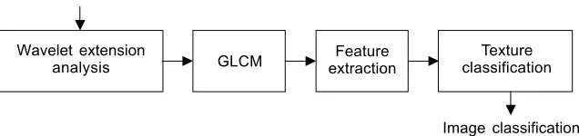
The proposed defect detection problem consists of two stages: (i) The feature extraction part which first utilizes the wavelet extension procedure to decompose textured image into four sub-bands and gray level co-occurrence matrix computed: energy, entropy, contrast and inverse difference moment for each sub-bands (ii) The detection part (texture classification) which is a mahalanobis distance classifier being trained by defect free samples (see Figure 2).

2.1 Review of Wavelet Transform

Wavelets are families of functions generated from one single prototype function, called the mother wavelet ψ (t) by dilation and translation operation. The wavelet basis is then provided by the function [9-11].

( ) / 2

(

)

, 2 2

j j

j k n n k

ψ = ψ − (1)

The mother wavelet is constructed from the so-called scaling function φ (t), satisfying the two-scale difference equation

( ) 2 ( ) (2 )

m

n h m n m

φ ∞ φ

=−∞

=

∑

Then, the mother wavelet ψ (n) is defined as:

( ) 2 ( ) (2 )

m

n g m n m

ψ ∞ φ

=−∞

=

∑

Figure 2 General flow process in identifying an echocardiography image

Input image

Wavelet extension

analysis GLCM

Image classification Texture classification Feature

where g(m) = (–1)m h(1 – m). In the wavelet literature, several different sets of coefficient

h(m) can be found, which are used to build a unique and orthonormal wavelet basis. Equation (2) and (3) can be generalized for successive spaces of approximation

c_j(k) and detail d_j(k) as follow:

( ) ( ) ₁(2 )

j j

m

c k =

∑

( ) ( ) ₁(2 )

j j

m

d k =

∑

The wavelet model can be generalized to any dimension. In the particular case of separable multiresolution approximation, the 2-D scaling function can be expressed by the product of two one-dimensional (1-D) scaling functions [5, 12]

(

)

φ =φ φ (6)

and the 2-D wavelet basis functions can be expressed by separable products of functions

φ and ψ as:

(

)

(

)

(

)

x y x y

x y x y

x y x y

n n n n

n n n n

n n n n

(7)

The corresponding 2-D h and g filter coefficients are separable

( )

( )

( )

( )

h k l h k h l h k l h k g l h k l g k h l h k l g k g l

= = = =

(8)

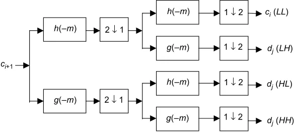
where the first and the second subscripts denote the low-pass and high-pass filtering characteristics in the horizontal and vertical direction, respectively. Figure 3 shows how to implement the wavelet decomposition step of two-dimensional (image) discrete wavelet transform (DWT).

In this research, a procedure called wavelet image extension is used. Wavelet image extension transform was developed by Mojsilovic′ et al. [5] and Neškovic′ et al. [6] which can be applied as an analyzing tool when the input samples are of small dimension. Starting from the original signal c(k), successive sequences of approximation

_{( ) 1( )}

( ) 2

j j

m

c k =

∑

_{( ) 1( )}

( ) 2

j j

m

d k =

∑

where h(m) =h(–m) and g(m) =g(–m). This decomposition can be seen as the passing

of the signal c_j+1(2k + m) through a pair of filter iH and Gi, (with the impulse response

h(m) and g(m)), and sub-sampling the filtered signals by two (dropping every second sample at the filter output).

Figure 3 Decomposition step of two-dimensional DWT c_i+1

h(–m)

g(–m)

h(–m)

2 ↓ 1

2 ↓ 1

g(–m)

h(–m)

g(–m)

1 ↓ 2

1 ↓ 2

1 ↓ 2

1 ↓ 2 _d

j (HH)

d_j (HL)

d_j (LH)

c_i (LL)

Using an appropriate set of wavelet basis functions, the original image decomposes into four frequency channels with the same resolution (i.e., the same number of samples). Using Equation (8) can be expressed:

( ) ( , ) * ( , ) ( , ) * ( ) ( )

( ) ( , ) * ( , ) ( , ) * ( ) ( )

( ) ( , ) * ( , ) ( , ) * ( ) ( )

( ) ( , ) * ( , ) ( , ) * ( ) ( )

LL

j j j

LH

j j j

HL

j j j

HH

j j j

c LL c x y h x y c x y h x h y

d LH c x y h x y c x y h x g y

d HL c x y h x y c x y g x h y

d HH c x y h x y c x y g x g y

⎡ ⎤

= = _{⎣ ⎦}

⎡ ⎤

= = _{⎣ ⎦}

⎡ ⎤

= = _{⎣ ⎦}

⎡ ⎤

= = _{⎣ ⎦}

(11)

frequencies (vertical details), and d_j(HH) the high frequencies in both directions (corner).

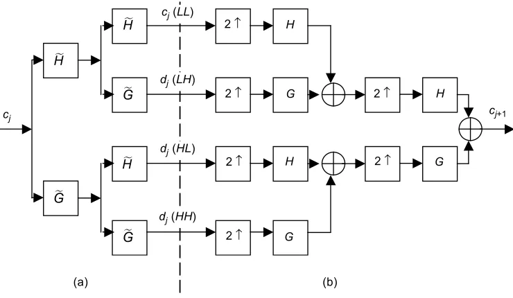
These four images are used as the input into the extension (interpolation) procedure, which is illustrated by the block diagram in Figure 4(b). As in the standard reconstruction procedure, we insert columns of zeros between successive columns of the images, convolve the rows with the corresponding 1-D filter, insert rows of zeros between rows of the resulting image, and convolve the columns with another 1-D filter, obtaining a new image with four times the pixels in the input image. The result of the complete decomposition extension procedure applied to one representative ultrasound image of a human heart is shown in Figure 5.

2.2 Co-occurrence Matrices

The co-occurrence matrix is defined by a distance and an angle, and its mathematical definition is

[ ]

_{

[ ] [ ]

[

]

_}

d

P i j = r c I r c =i I r+dr c+dc

where d be the displacement vector (dr, dc) specifying the displacement between the pixel having values i and the pixel having value j, dr is the displacement in rows

Figure 4 Block diagrams illustrating the complete wavelet decomposition-extension procedure (a) the composition part and (b) the extension (synthesis) algorithm

(a) (b) H~ H~ H~ G~ G~ G~ H H G G H G 2? 2? 2? 2? 2? 2? cj(LL)

dj(LH)

dj(HL)

dj(HH)

cj cj+1

cj

H

c_j+1 cj (LL)

d_j (LH)

dj (HL)

d_j (HH) 2 ↑

G H

G

2 ↑

2 ↑

2 ↑

2 ↑

2 ↑

(downward) and dc is the displacement in columns (to the right) and I denote an image of size N × N with G gray values [13].

Texture classification can be based on criteria (feature) derive from the occurrence matrices.

(i) Entropy

( )

( )

i j

ENT = −

∑∑

(ii) Contrast

(

) ( )

,

i j

CON =

∑∑

(iii) Angular Second Moment

( )

{

}

,

i j

ASM =

∑∑

(iv) Inverse Difference Moment

(

)

( )

1

, 1

i j

IDM p i j

i j =

+ −

∑∑

3.0 APPLICATION OF TEXTURE ANALYSIS

The proposed method for application of texture analysis system in echocardiography images consists of two stages:

Figure 5 The result of the complete decomposition extension procedure for one representative ultrasound image of a human heart. (a) Original image (b) After the decomposition (c) Synthesized (reconstruction) image with two times higher resolution

(i) The feature extraction phase, and (ii) the classification phase.

3.1 Procedure in Feature Extraction Part

Step 1: Given an original image c_j(m, n) of size M × N, decompose the image

c_O(m, n) at the original resolution (j = 0) into four sub-bands to obtain images,

c_O(LL), d_O(LH), d_O(HL) and d_O(HH) (having the same resolution). Step 2: Calculate the energy E_O for the original image, as well as the energy values

for E_O(LL), E_O(LH), E_O(HL), and E_O(HH). These values will be used as the first five components of feature vector x.

( ) ( ) ( ) ( )

[

]

= E EO O LL EO LH EO HL EO HH x

where the energy is computed by the formula:

( )

1 1

1

,

M N

j j

x y

E P x y

M N _{= =}

= ⎡_⎣ ⎤_⎦

×

∑∑

Step 3: Using the four images as input to the extension procedure, form a new image

c_j+1 = c₁ at the resolution j= 1, having twice the resolution of the input image. Step 4: Decompose the obtained image into the corresponding frequency channels

c_j+1(LL), d_j+1(LH), d_j+1(HL), and d_j+1(HH); calculate the energies E_j+1,

E_j+1(LL), E_j+1(LH), E_j+1(HL), and E_j+1(HH) and append these values to the feature vector x.

Step 5: Repeat Steps (3) and (4). The criterion to stop further extension could be the difference between the energy of an image with resolution j and the image with resolution j + 1. If the constraint

1

j j

j E E E

E ε

+

−

∂ = <

is not satisfied, the extension procedure should not be further performed because the energy values are significantly different.

Step 6: Construct the vector:

( ) ( ) ( ) ( )

+ + + +

= ⎡_⎣cj 1 LL dj 1 LH dj 1 HL dj 1 HH ⎤_⎦

j

c

Step 7: Derive the co-occurrence matrices _θO_,

d

P for d=1 (pixel separation distance) and angle θ = (0o, π/4, π/2, 3π/4) radians for each sub-band.

Step 9: Compute mean μ_k and standard deviation σ_k for each feature for four different angles are 0°, 45°, 90°, and 135°.

Mean μ_k is defined as:

1 1 , n k ik i x n μ =

=

∑

the standard deviation is

(

)

∑

n for k=LL, HL, LH and HH bands.

Step 10: Construct the vector

[

]

= Ent Ent Cont Cont Asm Asm Hom Hom

k,i

f

Step 11: Repeat Step (1) to Step (4) for all bands k (domain LL, HL, LH, and HH). Step 12: Feature extraction vector is constructed by the following vector:

[

]

= , , , ,

T LL i HL i LH i HH i

f f f f

i

s and for testing image

[

]

= , , , ,

T LL i HL i LH i HH i

f f f f

i

t

3.2 Procedure in Classification Part

Step 1: Compute covariance matrix C₁ and C₂ from feature vector s_i and t_i

respectively.

Step 2: Compute the mahalanobis distance d_i between each feature vector s_i and t_i, using equation:

(

)

(

)

1 2 _{1 2} 1 2

1 2

1 1

.

T i

d x x C C x x

n n

Step 3: Classify a testing image t_i for which d_i exceeds a threshold value α as defective or non-defective. α > ⎧ = ⎨ ⎩

infarcted area if

normal area otherwise

i i

d t

(

)

m q m

D D D

α = +η − (16)

D_m and D_q are respectively, the sample median and the sample interquartile of the order statistics. The interquartile range is the distance between the 75th and the 25th percentiles of the sample in image. D_i is obtained when distance d_i is arranged in ascending order and η is a constant determined experimentally.

4.0 EXPERIMENTAL RESULTS

The algorithms were developed and tested using MATLAB 7.0 release 14 along with Image Processing Toolbox, and Wavelet Toolbox [15]. As for hardware, Intel Pentium IV CPU 1.60 GHz, with 256 Mega-byte RAM and 20 Giga-byte capacity of hard disk were used. The echocardiography equipment used was the HP SONOS 5500 Imaging system.

All of the echocardiography images in this work have been obtained at Echocardiography Laboratory in Hospital Universiti Kebangsaan Malaysia, Kuala Lumpur. The connection process has been illustrated in Figure 6. The video sequence source from the echocardiography equipment is fed into the computer using Picolo Pro 2 frame grabber card. All input images saved into the PC are having similar quality. 8 frames image of every patient have been used as sample data for testing the accuracy of the developed algorithm.

For this purpose, asynergic segments were considered an infarcted area. Sample data were taken by supervised technician in cooperation with experienced echocardiographers. The experiments (training and testing phases) involved 17 patients. For each image to be analyzed, five tissue samples are taken from ultrasound image

Figure 6 Block diagram of the data acquisition system: (a) Echocardiography, (b) Personal computer (Data acquisition, storage, and display)

(a) (b)

Frame grabber Frame grabber

segments corresponding to area not affected by infarction, and five tissue samples are taken from image segments corresponding to suspected infarcted area. The size of the area are fixed to 16×16 pixels. Illustration of sample data taken from normal area and suspected infarcted area can be seen in Figure 1.

4.1 Texture Measure Result

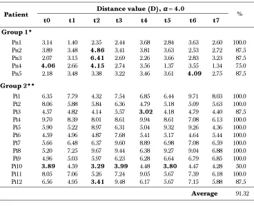
Results for the classification are shown in Table 1. Threshold value (α= 4.0) can be obtained by Equation (16). From this table, the highest accuracy performance obtained was 100%, for patients Pn1, Pi1, Pi2, Pi4, Pi5, Pi6, Pi7, Pi8, Pi9 and Pi11. The classification has a high performance if the input image is the easiest to identify from its alteration track from frame to frame. If the input image is of poor quality then the image may be wrongly identified. The lowest accuracy performance was patient Pi10 (50%) followed by patient Pn4 (75%). Overall accuracy for the classification results is

Table 1 Texture measure results for proposed method

Distance value (D), ααααα = 4.0 Patient

t0 t1 t2 t3 t4 t5 t6 t7

%

Group 1*

Pn1 3.14 1.40 2.35 2.44 3.68 2.84 3.63 2.60 100.0

Pn2 3.89 3.48 4.86 3.41 3.81 3.63 2.53 2.72 87.5

Pn3 2.07 3.15 6.41 2.69 2.26 3.66 2.83 3.23 87.5

Pn4 4.06 2.66 4.15 2.74 3.56 1.37 3.55 1.34 75.0

Pn5 2.18 3.48 3.38 3.22 3.46 3.61 4.09 2.75 87.5

Group 2**

Pi1 6.35 7.79 4.32 7.54 6.85 6.44 9.71 8.03 100.0

Pi2 8.06 5.88 5.84 6.36 4.79 5.18 5.09 5.63 100.0

Pi3 4.57 4.82 4.14 5.57 3.02 4.18 4.79 4.40 87.5

Pi4 9.70 8.39 8.01 8.61 9.94 8.61 7.08 6.13 100.0

Pi5 5.90 5.22 8.97 6.31 5.04 9.32 9.26 4.36 100.0

Pi6 4.59 4.96 4.87 7.68 5.41 5.17 4.64 5.44 100.0

Pi7 5.66 6.48 6.37 9.60 8.89 6.98 7.08 6.59 100.0

Pi8 5.20 7.25 9.67 9.44 6.38 9.27 9.04 6.88 100.0

Pi9 4.96 5.03 5.97 6.23 6.28 6.64 6.79 6.85 100.0

Pi10 3.89 4.59 3.29 3.99 4.48 3.80 4.47 4.28 50.0

Pi11 8.05 7.06 5.26 7.24 9.05 5.67 7.39 6.18 100.0

Pi12 6.56 4.95 3.41 9.48 6.17 5.67 7.15 5.88 87.5

Average 91.32

* Tissue samples taken from the normal area

91.32% using 136 samples data from 17 patients (125 correct and 11 incorrect). This result indicated that the algorithm is capable for identification of myocardial infarction tissue of heart from echocardiography images.

4.2 Comparison with Wavelet Extension Based on Energy

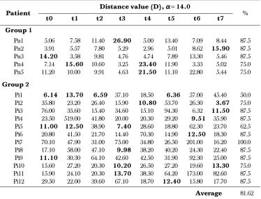
The performance of the proposed method was compared to that energy base of wavelet image extension transform based on energy [5]. For this comparison texture measure as input data were similar to that of the proposed method. The result for wavelet extension based on energy technique is presented in Table 2, the threshold value, α for this method is 14.00.

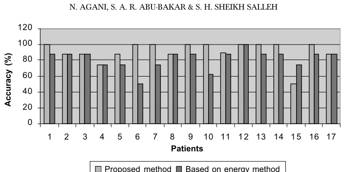
It can be seen that the classification rate obtained using the wavelet extension based on energy technique is 81.62%, while the proposed method has achieved 91.32%. The highest performance rate for the wavelet extension based on energy reached 100% by patients Pi7, while the lowest performance rate is 50% (Pi1). In general, the proposed method has shown better results than the wavelet extension based on energy

Table 2 Texture measure results for wavelet extension transform based on energy

Distance value (D), ααααα = 14.0 Patient

t0 t1 t2 t3 t4 t5 t6 t7 %

Group 1

Pn1 5.06 7.58 11.40 26.90 5.00 13.40 7.09 8.44 87.5

Pn2 3.91 5.57 7.80 5.29 2.96 5.01 8.62 15.90 87.5 Pn3 14.20 3.58 9.81 4.76 4.74 7.89 13.30 5.46 87.5 Pn4 7.14 15.60 10.60 3.25 23.40 11.90 3.33 5.02 75.0

Pn5 11.20 10.00 9.91 4.63 21.50 11.10 22.80 5.44 75.0

Group 2

Pi1 6.14 13.70 6.59 37.10 18.50 6.36 57.00 45.40 50.0

Pi2 35.80 23.20 26.40 15.90 10.80 53.70 26.30 3.67 75.0

Pi3 76.00 35.60 15.40 34.60 15.10 94.30 6.32 11.50 87.5

Pi4 23.50 519.00 41.80 20.00 20.30 29.20 9.51 35.90 87.5

Pi5 11.00 12.50 38.90 7.40 28.60 18.80 62.30 23.70 62.5

Pi6 20.80 41.50 21.70 14.40 70.30 14.90 12.50 18.30 87.5

Pi7 70.10 47.90 31.00 75.00 34.80 26.50 201.00 16.20 100.0

Pi8 17.10 58.00 47.10 9.98 38.20 40.20 24.30 22.40 87.5

Pi9 11.10 30.30 64.10 42.60 42.50 31.90 92.30 25.00 87.5

Pi10 15.60 27.20 20.30 10.20 26.50 27.20 19.60 13.30 75.0

Pi11 15.90 24.10 20.30 13.70 38.30 64.20 173.00 82.60 87.5

Pi12 29.50 22.00 39.60 67.10 18.70 12.40 15.80 17.70 87.5

method. Figure 7 shows the performance of each method in term of classification rates.

5.0 CONCLUSIONS

The combinations of the wavelet extension transform features with the gray level co-occurrence matrix have been proposed for application of texture analysis in echocardiography images. Its application is useful for a real world scene such as in biomedical field. The following conclusions can be drawn from our studies:

(i) Algorithm for texture analysis has the advantage of identifying myocardial infarction from echocardiography as normal tissue and infarcted tissue.

(ii) Wavelet extension and co-occurrence matrix procedure approach is an effective method for application in similarity evaluation of texture images.

REFERENCES

[1] Chang, T. and C. C. Jay Kuo. 1993. Texture Analysis and Classification with Tree-Structured Wavelet Transform. IEEE Trans. on Image Processing. 2(4): 429-441.

[2] Smith, J. F. 2004. Echocardiography. http://www.chclibrary.org/micromed/0046250.html. (Accessed on 30/06/2006)

[3] Kerut, E. K., M. Given, and T. D. Giles. 2003. Review of Method for Texture Analysis of Myocardium from Echocardiographic Images: A Mean of Tissue Characterization. Echocardiography: A Journal of CV Ultrasound & Allied Tech. 20(8): 727-736.

[4] Smith, J. F. 2004. Heart Attack. http://www.chclibrary.org/micromed/0046250.html. (Accessed on 30/06/ 2006)

[5] Mojssilovic′, A., M. V. Popovic′, A. N. Neškovic′, and A. D. Popovic′. 1997. Wavelet Image Extension for Analysis and Classification of Infarcted Myocardial Tissue. IEEE Trans. on Biomedical Engineering. 44(9): 856-866.

Figure 7 Performance of each method in term of classification rates

0 20 40 60 80 100 120

1 2 3 4 5 6 7 8 9 10 11 1 2 13 14 1 5 16 17

Accuracy (%)

p ro pos e d m ethod

Patients

[6] Neškovic′, A. N., A. Mojssilovic′, T. Jovanovic′, J. Vasijlevic′, M. Popopic′, J. Marinkovic′, M. Bojic′, and A. D. Popovic′. 1998. Myocardial Tissue Characterization After Acute Myocardial Infarction with Wavelet Image Decomposition. Cardiovascular Research Centre. Belgrade University Medical School. Belgrade University Faculty of Electrical Engineering. Institutes of Physiology and Pathology. Belgrade University Medical School. 634-641.

[7] Kim, N. D., V. Amin, D. Wilson, G. Rouse, and S. Udpa. 1998. Ultrasound Image Texture Analysis for Characterizing Intramuscular Fat Content of Live Beef Cattle. Ultrasonic Imaging. 20: 191-205.

[8] Agani, N., S. A. R. Abu-Bakar, and S. H. Sheikh Salleh. 2005. Texture Analysis of Echocardiography Images for Diagnosis of Myocardial Tissue. International Conference on Instrumentation, Communication and Information Technology. Bandung, Indonesia.

[9] Mallat, S. G. 1989. Multifrequency Channel Decomposition of Images and Wavelet Models. IEEE Transaction on Acoustics, Speech and Signal Processing. 37(12): 2091-2110.

[10] Daubechies, I. 1990. The Wavelet Transform, Time-Frequency Localization and Signal Analysis. IEEE Trans. on Information Theory. 36(5): 961-1004.

[11] Antonini, M., M. Barlaud, P. Mathieu, and I. Daubechies. 1992. Image Coding Using Wavelet Transform.

IEEE Trans. on Image Processing. 1(2): 205-220.

[12] Kim, N. D. 2000. Texture Representation Using Wavelet Filterbanks. Ph.D. Thesis. Iowa State University. [13] Amer, A. L., A. Ertüzün, and A. Erçil. 2000. An Efficient Method for Texture Defect Detection: Subband

Domain Co-Occurrence Matrices. Image and Vision Computing. 18(6-7): 543-553.

[14] Johnson, R. A. and D. W. Wichern. 1998. Applied Multivariate Statistical Analysis. Upper Saddle River, New Jersey: Prentice Hall.