Optimizing Effectiveness and Efficiency of Software Testing: A Hybrid Approach

(1)

BELL, KERA ZAKIYAH. Optimizing Effectiveness and Efficiency of Software Testing: A Hybrid Approach. (Under the direction of Dr. Mladen A. Vouk.)

The overall goal of software testing is to disclose defects efficiently (i.e. as little time and

cost as possible) and effectively (i.e. find as many faults as possible). It takes time to understand

what to test, to generate test cases, and to execute the test suite. It also takes time to analyze the

test results. In a situation where one can parameterize inputs and variables of interest, the cost of

generating random operational profile conformant test cases may be acceptable. It is typically O

(M×p) where p is the number of parameters and M is the number of test cases where a test case

is a vector of p values. However, random testing can result in very large test suites that may take

long to execute. Unless an automated oracle is available, results also may take long to analyze.

In contrast, systematic approaches tend to generate smaller test suites, thus reducing run-time and

analysis costs, but may take much longer to generate since they may require a higher-level of initial

expertise to develop. There may also be differences in the ability of various methods to detect faults

in the software. A question of interest is the following: Is there a way to take advantage of the

benefits of both statistical and systematic approaches in a hybrid scheme to optimize both efficiency

and effectiveness?

Hybrid approaches combine one or more testing techniques. This work discusses the

ba-sics of the underlying theory and presents the results of the associated experiments and simulations.

The specific parameter-based systematic technique is called N-wise testing. Test case vectors are

selected without replacement in N-wise testing. The N-wise technique assumes that most faults of

interest will be found when all or most of the involved parameter N-tuple values are covered by the

(2)

cases are sampled with replacement, and coverage of N-way faults is random. Thus it is not

guaran-teed that all N-way faults will be detected using random testing. However, a complete N-wise test

suite of M test cases guarantees that all N-way defects will be found. Given M random test cases

and M N-wise test cases, effectiveness of N-wise testing may be larger than that of random testing.

On the other hand, random testing may be more cost-efficient. The efficiency and effectiveness of

an approach that combines random testing with N-wise testing is explored.

In the case where all defects are N-way but one could only afford to perform k-wise testing

(k < N), a hybrid of k-wise systematic testing and random testing may help maximize efficiency

and increase effectiveness beyond that offered by either technique on its own. This hybrid approach

seems most effective when the minimum number of interacting parameters, N, required to expose a

defect is large and the average number of values associated with the p parameters is also large. A

potential use of hybrid testing is in testing for faults from failures that may result from a complex

combination of interacting parametric values, such as those found in security failures, and in testing

(3)

by

KERA ZAKIYAH BELL

A dissertation submitted to the Graduate Faculty of North Carolina State University

in partial fulfillment of the requirements for the Degree of

Doctor of Philosophy

COMPUTER SCIENCE

Raleigh

2006

Approved By:

Dr. Donald Bitzer Dr. Winser Alexander

Dr. Mladen A. Vouk Dr. Laurie Williams

(4)

(5)

Biography

(6)

Acknowledgements

(7)

List of Tables

1.1 Schools of Thought of Systematic Testing Versus Random Testing . . . 4

1.2 Example of Parameters and Associated Values . . . 9

1.3 Exhaustive Combinatorial Test Suite: All Possible Combinations of Parameters and Values . . . 13

1.4 Pairwise Test Suite: All Possible Pairs of Parameters and Values . . . 14

1.5 Random Combinatorial Test Suite Example . . . 15

3.1 Calculating the Maximum Number of Values Required to Use Random Testing Alone (v_max) . . . 37

D.1 CORPORATE Category of Vulnerabilities (a) . . . 85

D.2 CORPORATE Category of Vulnerabilities (b) . . . 86

D.3 CORPORATE Category of Vulnerabilities (c) . . . 87

(11)

List of Figures

1.1 The Objective of Software Testing is to “Break” Software . . . 2 1.2 Example of a Small Network Adding Complexity to a Testing - Note the Figure

Input Points are Marked A1, A2, A3 . . . 7 1.3 Example of a System with Many Inputs which can be Tested Simultaneously . . . 10

2.1 Effectiveness of Pairwise Testing in a Security Setting . . . 24 2.2 The Effectiveness of Pairwise Tests Based on Random Parametric Pairs (Relations)

and Pairwise Tests with Relations Based on Tester Expertise . . . 25 2.3 Comparison of CORPORATE1 Rate of Increase for the Number of Pairwise Tests

as the Number of Relations Increases . . . 27 2.4 Comparison of CORPORATE1 Number of Remaining Known Security Flaws as

the Number of Test Cases Increases . . . 28

3.1 Effectiveness vs Efficiency Comparing Hybrid Testing to 5-way Testing to Cover 5-Way Tuples within105_{Test Cases . . . .} ₃₉ 4.1 Rough Estimate of Guaranteed Coverage of Higher Order Tuples Using k-Way Tuples 43 4.2 Concept of Hybrid Testing used when Full t-Tuple Testing may not be Feasible . . 43 4.3 Comparison Schemes for Hybrid Testing (Minus Random Testing) and Random

(12)

Introduction

Software has proliferated over the years and has become more diverse, complex, and more recently network-based. Consumers indirectly or directly expect a certain quality of the software they use - whether in cars or airplanes they ride, at a check-out line where they make purchases, or when preparing their bank statements. To achieve quality that meets expectations, software must be tested. Properly testing software, especially critical software, is imperative. As one of the verification and validation methods, testing can help prevent catastrophic events and costly losses. This requirement is magnified in missions where software must operate for long periods of time and in environments where direct human intervention is not possible. There are a number of publications that discuss the present state of software testing [37, 84, 38, 39, 43, 22, 21, 55]. Different authors define software testing differently, but the consensus seems to include two things:

1. Software testing is a necessity to help attain any desired level of software quality [21, 50, 63, 43, 47].

2. The goal of software testing is to find problems (i.e. defects) in software so they can be addressed or fixed [22, 21, 63, 43, 47].

Finding software faults and defects before someone else (preferably before the release of that software) helps to prevent potential accidental or malicious exploitation of the faults. Testing is also used to pinpoint sources of software behavior(s) that perform contrary to what is expected.1

1_{In this text: a human error or mistake leads to introduction of a physical fault(s) into a software artifact. These initial}

(13)

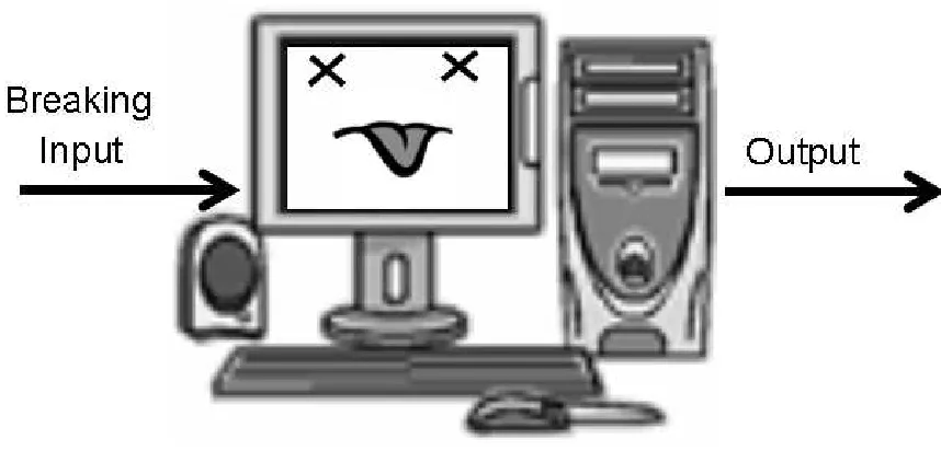
Figure 1.1: The Objective of Software Testing is to “Break” Software

Unfortunately, it is quite possible that expected behaviors may still be exploited in some way, which may not necessarily be based on any computer-related malevolence. While software testing is mov-ing from an art to a scientific process, it still has a long way to go [58, 55, 63]. More and more testing is driven by well-defined processes based on statistical and systematic testing approaches and automation is often a part of the solution. However, a lot of ad hoc nature and art remains when manual testing is used. The next several sections review some of the more common software testing approaches.

1.1 Software Testing Techniques

1.1.1 White-Box

White-box testing focuses on the internals of a system (also known as structural informa-tion). For example, one may exercise all possible branches or all assignment statements found in source code [34]. White-box testing often involves measurement of the extent of testing through “coverage” of the internal structures. When these structures are related to the faults and defects, this type of testing can provide stopping criteria and by name it is considered “good test-ing” [17, 50, 45, 62]. In practice, this type of testing seems to be most useful when structural information is not overwhelming and is readily available.

(14)

found in source code, is always available to a tester. Furthermore, a particular testing strategy may not always cover all faults of interest. In addition, existing white-box testing techniques tend to be time-consuming for large source codes [31]. While a good number of testing faults could probably be detected using white-box techniques, the amount of time needed to dedicate to this type of testing may be outside the constraints allotted to some particular software in practice [66].

1.1.2 Black-Box

Black-box testing, sometimes called functional testing, is concerned with inputs and as-sociated outputs of a system without regard to the internal structure of the system. In this context, a very useful concept is the operational profile of software under consideration [55]. An operational profile, in its simplest form, can be captured by the volume and relative frequency of usage of ex-ternally exposed software functions, operations, input variables, parameters, values, and states. An issue that may arise is how often and for what purpose may black-box test-driven sampling of the input space re-sample certain input states. In other words, black-box testing could result in a certain amount of redundancy in functional and input usage. In general practice, reuse of input states occurs and it is known as sampling of input spaces with replacement. During testing this may be inefficient It may take an exponential amount of exposure of software to testing or test operations (e.g., in terms of the number of test cases or in time) to reach a particular level of reliability that an end-user of software may require [66]. While any number of changes can impact and change the operational profile for which the software was designed, anticipatory testing for the related software input pa-rameter interactions becomes more challenging as software becomes more network-based, because distributed communications and networks can expose the software to totally new operational envi-ronments (and interactions) very rapidly and in an unpredictable way. New testing considerations may be required to ensure that testing remains sufficient as well as efficient.2

1.2 Categories

In this work we will group testing methods into one of the following two categories: systematic and statistical (or random) methods. Systematic testing is based on some set of guiding rules and a knowledge of structural and behavioral aspects of the software that are then translated into a targeted (often) non-random sampling of the software input space. On the other hand, random

2_{Most testers will use a combination of both white-box (structural) and black-box (functional) testing, in a practice}

(15)

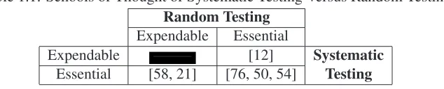
Table 1.1: Schools of Thought of Systematic Testing Versus Random Testing

Random Testing

Expendable Essential

Expendable ——– [12] Systematic

Essential [58, 21] [76, 50, 54] Testing

testing, as its name implies, uses random number generators to produce input data according to a pre-specified profile. For example, uniform random testing will sample all input values with equal weight, while operational profile based testing would sample the input space proportional to its usage in the field. Random testing is a software testing tradition.

It is possible to think of “classical” random testing as the use of minimal knowledge of an input domain to randomly select values for testing [80, 26, 61]. Minimal information may be environmental settings, input names, associated values, etc. On the other hand, according to some researchers, most systematic approaches can be considered instances of partition testing [61, 26]. “Classical” partition testing separates an input domain into disjoint sets or sub-domains based on certain criteria [5, 26, 61]. Each input of the sub-domain shares some specified trait(s) in common. In practice, there may be blurring of systematic methods and random methods when more complex operational-profile based testing is used.

There have been many debates over how to choose a particular partition testing approach and how partition testing compares with random testing. Many of these debates arise when a group of researchers believes random testing is not a good approach. Some researchers believe random testing is expendable, while systematic testing is essential and vice versa. Table 1.1 [34, 50, 5] cross-tabulates some of the papers found in different opinion domains.

It is not unusual to find a focus on statistical methods to help deal with test generation state space explosion issues [15, 55, 34]. The most common problem with statistical testing is that a large number of test cases may have to be generated before an adequate level of testing has been reached. While uniform random testing is the simplest approach, risk-tuned field-representative operational distributions are probably the most appropriate way of generating random test cases [55]. They tend to offer a summarized collection of information less detailed than that used for white-box testing but gives more internal information than black-box testing alone.

(16)

Preferences vary. Some like systematic techniques alone, and some prefer a combina-tion of both systematic and statistical techniques [55, 21]. Recent trends seem to lean towards approaches such as chaining, combinatorial approaches, counterexamples, behavior and data mod-elling, orthogonal arrays, control flow graphs, and others [68, 19, 53, 85, 17, 30, 29, 11, 69, 67]. For purposes of this discussion, systematic testing will be limited to combinatorial approaches.

1.3 Challenges in Software Testing

There are several major challenges that arise with testing modern software. Some are as follows:

• automation of the test case generation and their execution

• development of domain and software engineering expertise needed for adequate testing

• formalization and modelling of the software specifications and implementations, and software testing process and effects.

• the growing complexity of the modern software-based systems.

Good software testing is determined by the defined processes and their accompanying automated tools (if required), as well as the faults testing is able to discover, not the tools alone [63, 50, 54]. However, for introduction of new test generation techniques, it is important for automation to be possible as well. Manual testing can be cumbersome because it is tedious, time-consuming, and error prone [47, 21, 50, 62, 43].

On the other hand, some critical activities may require manual testing [50, 21]. Also, functions may only need to be tested once, and may therefore benefit from manual testing in terms of cost effectiveness [50, 54]. A tester should be cautioned since it is difficult to precisely repeat a manual test scenario. [21, 54]. Human error can become a factor if repetition is required [63].

(17)

Formal modelling is sometimes used to verify and validate software, and aid in testing through formal test cases and graphical representations. Models can take many forms: coverage models, control flow models, finite state machine models, etc. As software increases in complexity, such models, depending on the level of abstraction and detail used, may be a less realistic repre-sentation of a real system or may be difficult to understand. Because large systems usually have a large number of states, state explosion problem may restrict or hinder formal modelling in prac-tice [32]. In pracprac-tice there could be (and usually are) unexpected differences, states and scenarios not accounted for by the models [77].

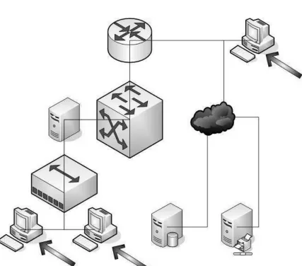
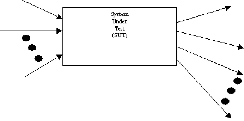
System and software complexity has dramatically increased as the hardware becomes more capable, as functionalities and expectations of customers grow, and the world becomes more networked. For example, network-based environments are usually nondeterministic since more than one path can be taken to achieve a particular outcome. Although “traditional” software may have a single entry point for input and/or data entered into a system serially, that often does not hold true for a large networking environment. For example, Figure 1.2 illustrates a simple network with three possible data entry points indicated by the arrows. Traditionally, one may consider one data entry point at a time. In a network setting, however, it is possible for two inputs or even all three to occur simultaneously. This adds to the complexity of the software under test in this environment.

While techniques for testing network-based software may involve a series of syntax-oriented operations, in actual operation there may be a number of things that can go wrong that have very little to do with input parameter syntax faults, but a lot to do with complex interactions among the input and environmental parameters. Therefore, it is important to extend testing philosophy to more complex notions of semantics and correlated events and operations. For instance, a number of security violations can take place through memory abuse - often the result of a time-correlated series of unexpected or improperly tested operations or events, through correlated disturbance of estab-lished connections - such as spoofing [87]. Unfortunately, some of the catalysts for these problems may not be known a priori [77].

1.4 Random Testing

1.4.1 Advantages

(18)

Figure 1.2: Example of a Small Network Adding Complexity to a Testing - Note the Figure Input Points are Marked A1, A2, A3

implement and can generate a complete test suite rather quickly. Typically, inO(v×M)for random testing with replacement where v is the total number of values in the space and M is the total number of test cases orO(p×M2₎_{for random testing without replacement where p is the number} of parameters and M is the number of test cases. According to Lewis, random testing can sometimes catch defects that systematic processes could possibly miss [50], especially when operational profile distribution is used in testing [55].

1.4.2 Issues

(19)

direct measure of reliability [21, 55]. Furthermore, some researchers feel that less systematic strate-gies tend to have lower confidence bounds [80, 21], and random testing could result in wasted effort. One reason is that in practice random testing is often done with replacement so that there are re-peated test cases [21]. It also may take time to ascertain correctness of the output (the “oracle” issue) and pinpoint the source of a problem using this technique. Craig and his colleagues claim that random testing offers little in terms of reliability since risk cannot be directly measured and coverage is not well-defined [21]. Some employ brute force testing based on uniform distributions while others have used more weighted distributions, such as an operational profile [55]. Another is-sue with random testing is that, unless a tester knows the precise random generating functions used, repeatability may become an issue which could affect potential automated activities [50, 21, 54]. Random testing may suffer from similar problems manual testing does. A decrease in automation could mean a decrease in effectiveness [54]. However, some supporters of systematic testing ar-gue that these semi-random techniques do not provide additional function coverage over systematic techniques [21].

It has been reported that random testing alone may find, “. . . only one out of every three errors present in the software,” [54] and those errors may be part of that 1/3 defects that systematic processes may miss [50]. It seems that very few studies would suggest performing random testing alone to effectively catch defects [54, 61, 50].

On the other hand, there are authors who believe that reliability can effectively be im-proved and estimated using random testing [12, 68, 55, 80].

1.4.3 An Example

Suppose that the testing space shown in Figure 1.2 can be expressed as a collection of parameters and their associated values based on the data entry points indicated by the arrows. For-mally, this space reading left-to-right can be represented asA1,A2andA3where1≤i≤3andAi is an input parameter.

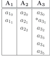
Let Table 1.2 represent a list of parameters (A1, A2, A3) with their associated values listed underneath. Each subscript is the associated parameter and each sub-subscript represents an enu-merated value for that particular parameter. Assume that an ‘off’ state exists for every parameter. Without loss of generality, we can assume that the first value represents an ‘off’ state (i.e. ai0 is off).

(20)

Table 1.2: Example of Parameters and Associated Values

A1 A2 A3

a₁₀ a₂₀ a₃₀ a11 a21 *a31

a22 a32 a₃₃ a34 a35

unique executions possible. Suppose a defect could be detected whena11is executed or whena31is executed (indicated by the ‘*’). There is a 2/11 chance of finding the indicated defects in one trial. How many trials would minimally be required to attain a probability of more than 1/2? Probability is f = 1-2/11 of not detecting the problem in one attempt. Assuming that the space is sampled with replacement (which in this case is really not the best option), and (assuming independence of the trials) f to theMth_{power is the probability of not detecting a problem in M trials. Hence, solving} Equation 1.1 for M will compute the expected minimum,Mmin(Equation 1.2). In this case, at least 4 test cases would need to be executed to hit at least one of the defects with probability of 1/2. If a 99.99% chance of finding at least one defect is desired, then one would need to execute at least 46 test cases. However, in this case, exhaustive testing means the execution of all single values, which would be 11 test cases. Obviously, sampling with replacement is very inefficient since executing just 11 test cases (without replacement) would find all problems. As the input space grows (in terms of a large number of parameters and values), the situation may change.

1−

µ

1− 2 11

¶_M > 1

2 (1.1)

Mmin =

   log

³

1− 1₂´ log³1−₁₁2´+ 1

  

 _(1.2)

1.5 Combinatorial Testing

Single-input executions were discussed in the Section 1.4.3 example. There are situations in which a number of parameters interact and can be (and should be) tested simultaneously.3 An example of a system exhibiting this behavior can be seen in Figure 1.3. In this situation, there are a number of combinations among input parameters that can exist. Assume that one parameter can take

(21)

exactly one value at any given instant.4 _{Generating test cases based on combinations of parameter}

values is commonly referred to as combinatorial testing. Exhaustively testing everything, (i.e., all combinations) often leads to a combinatorial (state) explosion.

For example, let a system have 20 parameters and 5 possible values for each, then there would be520_{or 95,367,431,640,625 possible combinations. To put this into perspective, if one test} case takes 1µs to test, then the entire suite would take approximately 3 years to execute! This may be an acceptable time frame for some systems, but in other situations - such as rapid testing - testing needs to be completed within months if not weeks [22].

There is ample research on this type of testing and how to intelligently reduce the number of tests that arise in a combinatorial environment [12, 68, 19, 17, 86, 85, 90, 53, 49, 8, 7, 9, 10]. One such systematic technique is called N-wise testing. The randomly generated counterpart of N-wise testing is called random combinatorial testing [68]. In random combinatorial testing at least two inputs are tested simultaneously.

Figure 1.3: Example of a System with Many Inputs which can be Tested Simultaneously

4_{If a parameter can assume more than one value at a time, that parameter can be split into more than one parameter}

(22)

1.5.1 N-wise Testing

N-wise testing is a systematic technique which ensures that all possible combinations of the values of N parameters appear in a test suite at least once. N is a positive integer in the range 2≤N ≤pwhere p is the total number of parameters of the system under test.5 N-wise testing is generally used in cases where systems have at least 2 parameters and at least 2 values per parameter. This testing guarantees that all possible N-tuples are covered in the test suite at least once [17, 75]. Naturally, N can vary but cannot exceed the total number of parameters. N-wise testing has been shown to be NP-Complete [49], so algorithms performing this type of testing are based on heuristics, and there is much research dedicated to deciding how to perform N-wise testing [17, 85, 49, 53, 75].

1.5.2 Advantages and Disadvantages

An advantage of combinatorial testing is that it is designed to meet the needs of systems with a number of parallel inputs. This type of testing can result in a relatively small test suite, especially if the N-way combinations are sampled without replacement. Several studies have found this to be effective [19, 12, 68]. Pairwise testing (and N-wise testing in general) has been shown to be fairly effective with some types of software systems and may prove beneficial for testing other types of systems [19]. An unfortunate recent example of a software-related loss, which might have been prevented by exploring relationships among different input and environmental parameters related to the operation of the system as a whole, is the case of the NASA Mars Climate Orbiter. It crashed onto the surface of Mars because of a mismatch in the measurement units assumed for input data and those expected by the navigational software. The estimated loss was $165 million dollars [40]. This failure was a direct result of inadequate relationship interaction testing of the system parameters.

One of the pitfalls of performing combinatorial testing is the classification of parameters. Such an activity may be relatively easy when performing configuration testing where the parameters are pre-defined. However, in complex systems deciding to group certain behaviors together is a non-trivial task. Although most researchers have attempted to make such groupings disjoint, it has been suggested that this may not be possible [70]. Another problem is that although non-exhaustive combinatorial testing, such as pairwise testing, has been shown effective with some systems, there may be situations in which one may not choose to use this technique. [72] Smith et al. reported that

(23)

many critical defects apparently missed in one of their systems using pairwise testing. Hence, there is a need to join combinatorial testing with other techniques to provide a more complete coverage of the software fault-space.

1.5.3 Example

A test suite can be represented as a single parameter, two parameters, or all parameters. Letaij represent thejth value of parameterAi. In general, the exhaustive combinatorial test suite

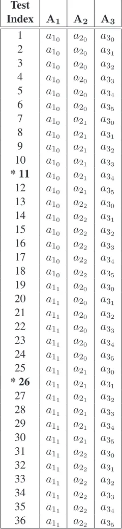
could formally be represented as a Cartesian product{(A1 ×A2×A3)}of all possible values as shown in Equation 1.3. Based on the example given in Table 1.2, there are a total of2×3×6= 36 possible combinations when all parameters are considered to interact with each other. One possible combination is (a₁₀,a₂₁,a₃₅). All possible combinations are shown in Table 1.3.

Exhaustive Suite={(a1i₁, a2i₂, a3i₃) : (1≤i1≤ |A1|),(1≤i2≤ |A2|),(1≤i3≤ |A3|)}

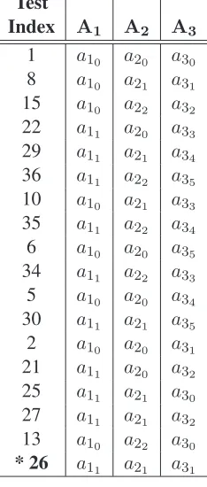
(1.3) Consider the example in Table 1.3, which could also be considered 3-wise exhaustive testing. Table 1.4 shows a test suite that would satisfy N = 2 or pairwise testing. Table 1.4 is smaller since there are 18 test cases total; and all that is required is that each pair of parameters appear at least once in the suite. Notice that there could be more than one possible pairwise test suite.

(24)

Table 1.3: Exhaustive Combinatorial Test Suite: All Possible Combinations of Parameters and Values

Test

Index A₁ A₂ A₃

1 a₁₀ a₂₀ a₃₀

2 a10 a20 a31

3 a10 a20 a32

4 a₁₀ a₂₀ a₃₃

5 a10 a20 a34

6 a10 a20 a35

7 a₁₀ a₂₁ a₃₀

8 a10 a21 a31

9 a10 a21 a32

10 a₁₀ a₂₁ a₃₃

* 11 a10 a21 a34

12 a10 a21 a35

13 a₁₀ a₂₂ a₃₀

14 a10 a22 a31

15 a10 a22 a32

16 a10 a22 a33

17 a10 a22 a34

18 a10 a22 a35

19 a11 a20 a30

20 a11 a20 a31

21 a11 a20 a32

22 a11 a20 a33

23 a11 a20 a34

24 a11 a20 a35

25 a11 a21 a30

* 26 a11 a21 a31

27 a11 a21 a32

28 a11 a21 a33

29 a₁₁ a₂₁ a₃₄

30 a11 a21 a35

31 a11 a22 a30

32 a₁₁ a₂₂ a₃₁

33 a11 a22 a32

34 a11 a22 a33

35 a₁₁ a₂₂ a₃₄

(25)

Table 1.4: Pairwise Test Suite: All Possible Pairs of Parameters and Values

Test

Index A1 A2 A3

1 a10 a20 a30

8 a10 a21 a31

15 a₁₀ a₂₂ a₃₂

22 a11 a20 a33

29 a11 a21 a34

36 a₁₁ a₂₂ a₃₅

10 a10 a21 a33

35 a11 a22 a34

6 a₁₀ a₂₀ a₃₅

34 a11 a22 a33

5 a10 a20 a34

30 a11 a21 a35

2 a10 a20 a31

21 a11 a20 a32

25 a11 a21 a30

27 a11 a21 a32

13 a10 a22 a30

* 26 a11 a21 a31

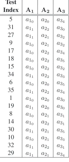
of redundant tests. Table 1.5 illustrates a test suite based on random selection ofM = 183-way test cases from the exhaustive suite without replacement. This test suite hits one of the failing test cases, exhaustive number #26, on the18th_trial.

1−

µ

1− 1 18

¶_M > 1

2 (1.4)

M_min =

   log

³

1− 1₂´ log³1−₁₈1´+ 1

  

 _(1.5)

1.6 Testing Network-Centric Software

(26)

Table 1.5: Random Combinatorial Test Suite Example

Test

Index A1 A2 A3

5 a10 a20 a34

31 a11 a22 a30

27 a₁₁ a₂₁ a₃₂

9 a10 a21 a32

17 a10 a22 a34

18 a₁₀ a₂₂ a₃₅

15 a10 a22 a32

34 a11 a22 a33

6 a₁₀ a₂₀ a₃₅

35 a11 a22 a34

1 a10 a20 a30

19 a11 a20 a30

8 a10 a21 a31

14 a10 a22 a31

30 a11 a21 a35

10 a10 a21 a33

32 a11 a22 a31

29 a11 a21 a34

during its operation.

There are many factors that play a role in the way software is tested. Resource constraints are often the primary driver (deadlines, personnel, cost, etc.). For instance, it is often impractical to test every permutation of all possible inputs (also known as a combinatorial exhaustive test). Unfor-tunately, a potential problem with selecting a sub-group of exhaustive tests is that a high risk defect could go undetected. Research shows that important failures are frequently the result of unexpected and unusual combinations and interactions (often correlated over time) of many parameters, faults and error-states [84, 4]. Therefore, it is important to investigate techniques that can help expose the underlying faults and at the same time adhere to a set of resource constraints [82].

(27)

constraints. Pairwise testing [18, 75], enhanced with partial N-wise testing [7], may offer a vi-able option. The first step in making a case for the use of N-wise enhanced testing in the domain of unusual and unexpected failures and defects (such as security failures [77]), is to compare its effec-tiveness in that space with a technique such as random testing. Random testing is often used since it can be simple to implement and can be quite effective [4, 84, 12]. However, it has limitations [84]. For example, reliability analyses may be weak unless statistical coverage is guaranteed [5, 21]. The work reported in this chapter compares pairwise testing and random testing in the domain of network-centric software.

1.7 Motivation for Current Work

Random testing alone may not adequately test a system for faults, although it can be effec-tive in some instances [50]. It is commonly used as an “add-on” technique to enhance a systematic process [21, 50, 47, 22, 61]. In fact, in order to adequately test software, a systematic process must be in place [54, 21, 50, 47, 22]. Schroeder et. al. define the set of all possible combinations of test values asTcart which can be seen in Equation 1.6 [68]. This is basically the Cartesian product of all possible values of each sub-domain. The size ofTcartcan be seen in Equation 1.7. On the other hand, systematic processes can be costly in terms of time and available resources and they may be certain types of faults that may be missed using a particular systematic process alone [21, 50].

In a highly complex environment, such as network-based system, it may be too costly not to test the lower probability sub-domains. It may be beneficial to adopt a process which combines random and systematic testing in a way that takes advantage of the efficiency of random testing and the effectiveness of some type of systematic testing for the low probability sub-domains. Unfortu-nately, there does not seem to be a consensus on how much random testing to perform vs. how much systematic testing to perform. Ntafos has suggested that both random and partition testing detect faults at about the same rate, except in the cases of “. . . low probability sub-domains that have high failure rates.” [61]

Instead of picking a systematic technique over a random technique, it may be profitable to find a way to combine both. Utilizing combinatorial techniques may provide a viable systematic process to do just that.

(28)

unusual or unexpected behaviors, such as security flaws. This testing could be also quite cost efficient since test suites grow linearly with the number of parameters when N is relatively small.

Tcart={D(x1)×D(x2)× · · · ×D(xN)} (1.6)

|Tcart|=|D(x1)| × |D(x2)| × · · · × |D(xN)| (1.7)

Some important questions in that context are:

1. Is there a way to effectively and efficiently combine random testing and systematic testing?

2. Is there a way to determine the amount of effort required to perform a systematic process if random testing is performed first?

3. Is there a way to determine the amount of effort required to perform random testing if a systematic process is performed first?

4. Is there a way to effectively and efficiently combine various types of systematic testing into one process?

5. Is it worthwhile to use statistical analysis from a systematic profile to perform this type of testing?

1.8 Dissertation Outline

(29)

Chapter 2 Testing in Complex Environments

Modern networking environments add a new and very complex component to most mod-ern software-based systems. Interfacing over networks not only makes verification and validation of such software more complex, but it also makes such systems vulnerable to network-borne se-curity attacks if one of the residual faults is exploitable via a network. Network-related sese-curity failures, but also other problems, can result from unusual and unexpected relationships among soft-ware/system parameters - input, output, internal and operational environmental parameters. De-signer and tester expertise alone may not be sufficient to expose such exploits. This chapter inves-tigates the issue of how to test for both normal and unusual relationships among software param-eters in a systematic fashion, especially those related to complex relationships, such as network-associated operations. It also looks into problem-detection effectiveness of the approach. In this context, it explores methodologies, fault-detection, and cost effectiveness of different variants of a technique called N-wise testing.

2.1 Using N-wise testing

(30)

(i.e. 2-way testing) [68]. Of course, it is possible that higher-order (N-tuple) interactions, e.g., 5-tuple interactions, are needed to discover a fault and that such an interaction may appear by accident in a pair generated test-suite. If certain fault-types are known to require a high-order interaction for detection, it may be advisable to guarantee coverage of more N-way constructs for anN >2.

Cohen and his colleagues were able to implement N-wise testing techniques on practical systems using heuristics [17]. Dalal and Cohen analyzed same-sized random test data sets and found them to cover a very high percentage of input pairs; as high as 90% in many cases [18, 19, 17]. Schroeder et al. define fault detection effectiveness (FDE) as the percentage of faults detected by a testing technique when executed on a system with known fault content [68]. Based on these hypothetical cases, one may not expect the FDE of pairwise and the random test data sets of the same size to vary a great deal.

Bolaki recently compared pairwise (and N-wise) testing techniques against random test-ing techniques [12]. He performed studies on two software systems that have been used in prac-tice. One is called the Data Management Analysis System (DMAS), which is utilized by analytical chemists for data processing. The second is called the Loan Arranger System (LAS), which is used as a support system for mortgage-backed security businesses. He parameterized the inputs for both systems. More details regarding Bolaki’s work can be found in Appendix E.) Of interest is what we call the defect degree, i.e., is the defect an 3-way, 5-way, and in general a k-way defect. That is, what is the minimum number of interacting parameters required to detect a particular fault or defect. This information is important since it tells us what level of N-way testing is needed to achieve a certain comfort level with respect to adequacy of the testing. Some of that information was not available in Bolaki’s work, so it was derived. This is discussed further in one of the later subsections. Once Bolaki parameterized the systems, he used fault seeding to create faulty versions of the correct software one line at a time based on a particular fault model. According to Bolaki, only “simple” faults were injected into each system respectively. Bolaki then used an automated tool called the “Test Vector Generator” to construct the test suites based on particular criteria such as N-way relations, random, etc. He found that when the number of values per defined parameter is between 2 and 3 (on the average), random testing performs just as well as N-wise testing.

(31)

of interacting parameters required to detect a defect was greater than 3, and the maximum number of values associated with one parameter was 10. The maximum number of parameters required to expose a defect was 4, which occurred about≈10% of the time. Because of suite size limitations, some of these configurations may never be exercised using random testing techniques.

On the other hand, and this is not surprising, there are indications that in practice N-wise testing has limitations. In testing Remote Agent Experiment (RAX) software used to control NASA spacecraft, Smith, et al. [73, 68] present their experience with N-wise testing. Their analysis indicates that pairwise testing detected 88% of the faults classified as correctness and convergence faults. Depending on the safety and cost criticality, this percentage may or may not be acceptable. Only 50% of the interface and engine faults were covered, which would be considered poor coverage for this type of system. Higher orders of N-wise testing could possibly find more faults where 2< k≤N.

2.2 Assessing N-Wise Approach for Security Testing

Security issues and faults related to those issues are a subset of all other faults/flaws. However, security-related faults usually carry a higher risk factor and often arise as a result of potentially unforeseen dependencies, relationships, interactions, and constraints among the known system parameters [77]. The driving question is whether one can devise a formalized, systematic testing approach that allows automatic generation of test cases which cover ‘unexpected’ parameter interactions. Also of interest is the cost-effectiveness of the approach in terms of the number of test cases and in terms of finding security flaws.

N-wise testing offers a promising approach to this problem. It is important to determine the level of N-wise testing necessary given thatN >2testing may considerably increase the com-plexity of the process and the number of test cases. The useful value of N can be determined a number of ways. One way is presented in the chapters that follow. All N-wise testing methods start out by assuming that all parameter groupings are independent of each other. Heuristics are then used to generate a suite of test cases that cover the N-tuple space.1 _{These tests are then modified}

by explicit specification of inter-parameter dependencies and constraints [19, 75]. This tends to increase the number of test cases to provide additional coverage required by the relationships

(dis-1_{The In-Parameter-Order method [49] was used as the N-wise testing heuristic throughout this dissertation. An}

(32)

cussed later in this chapter). Still, the number of test cases generated that way is far smaller than when all possible combinations of parameters are tested. This approach is also more repeatable and more likely to be automated than ad hoc approaches based on tester expertise. However, one would like to know the level of expertise that is required to produce appropriate N-wise relationships and constraints that provide similar or better fault (or flaw) coverage when compared to good ad hoc testing, good random testing, or testing using some other systematic approach. This is especially interesting in environments where ‘unexpected’ operational profile changes and bursts are the order of the day. An example of such an environment could be one which employs a network and depends on message communication. Unexpected changes and bursts could be the result of a number of things, such as malicious security attacks.

2.2.1 Data

The general approach taken in this part of the study is the following one. A set of known security flaws/problems/faults were collected from a public data repository at the Secure Space site [28].2 _{Those flaws were then parameterized, i.e., the conditions and inputs needed to describe}

the flaws were broken down and turned into failures based on individual parameters and associated parameter values. A set of parameterizations is show in Appendix D. Next those parameters were used to generate test cases using different parameter-based testing approaches - specifically N-wise method, random method, and expertise method. Finally, both the fault finding ability (effective-ness) of the different methods and the effort, number of test cases, and the algorithmic complexity (efficiency) needed to find the faults were compared.

The collection of known security flaws reported on-line for network-based devices [28] consisted of two sets of data. One set of 52 security flaws was reported in the database for switching devices from October 26, 2000 to June 9, 2004. Appendix D lists the 52 problems along side the risk level, flaw ID number, date of recording, and the prarmeterization applied to it. A more detailed description of each individual fault can be found at the Secure Space web site.

We used 47 of 52 faults to form a data set we call CORPORATE1. We also formed an-other set, which we call CORPORATE2, again using data from the Secure Space web site, that contained 23 flaws pertaining to a firewall category3. The published flaws were parameterized in the flaw space, and not in the platform space, i.e., the platform details were in most instances sim-ilar and were ignored to reduce the number of relatively-invariant parameter values. Then we used

(33)

a tool called PairTest (Version 1.1) [14, 75] to generate test cases with different relationship and constraining strategies. For example, in one part of the study (described further in a section that follows) tester-driven pairwise test cases were developed for 55 parameters from CORPORATE1. Also, random relationships (mutual exclusivity of values and correlation of parameters) were auto-matically generated using our toolset. In this particular case, random relations were generated for pairs of parameters. Any parameters not explicitly included in the pairwise relations were guaran-teed one-way coverage only. This means that every parametric value was guaranguaran-teed to appear at least once.

2.3 Detecting Security Faults

2.3.1 Transitivity

Security flaws are often exploited as a result of factors and relationships unknown at the time software is developed[77]. Therefore, it may not be sufficient to base security-related software testing and relational pairing rules on tester expertise alone. It may be worthwhile to investigate the effectiveness of an approach where relationships are randomly generated assuming pairwise [75], or N-wise in general, dependencies among different groupings of application parameters.

One goal was to determine the effectiveness of disclosing known security flaws using N-wise testing when dependencies amongst specified parameters are randomly chosen. Another goal was to determine the effectiveness of disclosing security flaws outside the space of known security flaws, i.e., to define parameters on one set of flaws and measure how effective that test suite is on another set of security flaws.

The latter resulted in an interesting observation on transitivity of effectiveness (ability to find faults) of pairwise testing under different strategies for generation of relationship rules and constraints. Pairwise test cases and relationships were generated using the extended version of the PairTest tool.

(34)

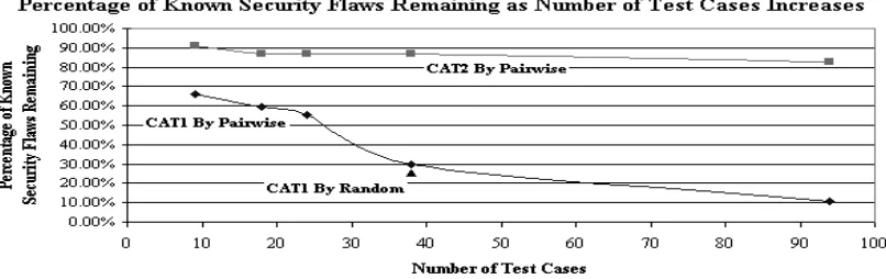
of the total number of test cases generated using the CORPORATE1 flaw-set as the basis. The first point is for 9 test cases generated assuming total independence of CORPORATE1 parameters. This one detected only about 30% of the flaws. The second and third points are for test cases generated based on 10 and 20 random relationships, respectively. The fourth point is 38 test cases based on 30 general relationships created through human (tester) expertise rather than random generation of relationships. Detection rate increased to about 70%. Final point on CAT1 curve is the one where relationships were generated through ”full expertise” of a human tester. “Full expertise” refers to using only the tester’s knowledge to formulate a test suite, which is a form of ad hoc testing. The application of “full expertise” of the author (64 relationships, 94 test cases) for this particular study increased the detection rate to about 90% or better.

A comparison of CORPORATE1 effectiveness of pairwise testing using 38 test cases and a random approach with the same number of test cases, shows that pairwise testing appears to be as effective as random testing with replacement. This confirms a recent finding by Bolaki [12]. This is good since the number of test cases needed to find problems with pairwise testing appears to grow slower than with random testing. It would also appear that application of expertise to the generation of these 38 random test cases may do as well (about 70% detection) as application of that expertise to produce 30 general relationships in the pairwise approach, so random testing with replacement seems to provide a lower bound for the effectiveness of N-wise testing.

Inspection of the relationships needed to detect flaws in the case of the CORPORATE1 data set indicates that, on average, the minimum number of parameters required to interact in order to detect a known security flaw was at least 3. This suggests that it may be necessary to routinely generate at least 3-way relations (and perhaps some of higher order) to adequately detect some security flaws.

(35)

Figure 2.1: Effectiveness of Pairwise Testing in a Security Setting

2.3.2 Expertise

Many current testing techniques may be effective when used properly. However, it has been shown that many testers lack the experience required to use them effectively [64]. Also, tools are sometimes difficult to learn and may not become fully integrated into a testing process. There is a need for techniques that both increase the ability to test for unusual combinations and at the same time compensate for possible tester inexperience to help increase the overall effectiveness of testing [25]. What is the role of expertise in the pairwise context?

Pairwise test cases were generated by progressively increasing the number of specific relationships and constraints. One has to distinguish between full N-way testing (generation of all N-tuples for a given full set of parameters) and 2-parameter testing, where all pairs are generated only for a subset (in this case in pairs) of the parameters, the rest being chosen randomly. When only pairs of parameters are used, then the relationship assumed between only the two chosen parameters and all pairs of values two particular parameters cover is guaranteed. The rest of the pairs may or may not be present, but all values are guaranteed to be there at least once.

When running test cases, relationships found in the test-cases are compared with com-binations of the parametric values in each flaw-case. For the CORPORATE1 set the interacting parameters are listed in the last column of Appendix D while the actual full set of parameters are listed in Appendix C. If there was a match between relationships in the test-case and relationships in the flaw/fault table, it was assumed that the fault was detected.

(36)

10

100

0

10

20

30

40

50

60

70

80

90

100 Percentage of Known Security Flaws Remaining

Number of Relations

Pairwise Test Cases with Tester Expertise

Test Cases with Random 2-Parameter Pairwise Relations

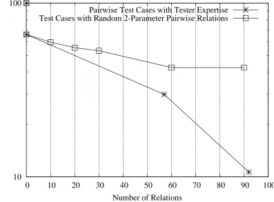
Figure 2.2: The Effectiveness of Pairwise Tests Based on Random Parametric Pairs (Relations) and Pairwise Tests with Relations Based on Tester Expertise

randomly or by hand, and the role of human expertise.

Figure 2.2 explores the issue further. The vertical axis is logarithmic and shows the per-centage of known flaws remaining (CORPORATE1 data set). The horizontal axis is the number of relationships generated in the tests. The first thing to note is that random generation of relations is less effective in finding problems than an expertise-driven test suite with a corresponding number of relations. This is not unexpected. However, the random approach has lower overhead than the expert-only approach.

(37)

manually generate 57 general relations based on one researcher’s expertise. It also took another 4 hours to extend the number of relations to 92. Using the randomly generated relations for pairwise testing could have resulted in over 300,000 automated test executions in the same amount of time it took to generate the relations by hand!

2.3.3 Random

There appears to be a definite advantage in using random relations and random testing for long runs, but it does take longer to find all the problems. If the cost of failure identification and fault repair is high, using fewer test cases may be a better option. On the other hand, the number of test cases generated by the random 2-parameter pairwise-relations process seems to increase at about the same rate as the number of test cases generated manually, but it would appear that the expert approach takes a somewhat straighter “path”. This can be seen in Figure 2.3. The figure shows the number of test cases generated for CORPORATE1 fault-suite versus the corresponding number of relations.

The expert approach and generation of random relations appear to have similar effective-ness, at least in the range examined here. This is shown in Figure 2.4, which plots the effectiveness of testing versus the number of test cases generated. The stopping criterion for the randomly gener-ated tests in this figure was the number of pairwise test cases genergener-ated.

(38)

10

100

0

10

20

30

40

50

60

70

80

90

100 Number of Test Cases

Number of Relations

Pairwise Test Cases with Tester Expertise

Test Cases with Random 2-Parameter Pairwise Relations

(39)

10

100

0

10

20

30

40

50

60

70

80

90

100 Percentage of Remaining Known Security Flaws

Number of Test Cases

Randomly Generated Test Cases

Pairwise Test Cases with Tester Expertise

Test Cases with Random 2-Parameter Pairwise Relations

(40)

Chapter 3 Hybrid Software Testing

Hybrid approaches combine one or more techniques. This chapter focuses on the effi-ciency and effectiveness of a testing approach that combines N-wise testing with random testing. Only discrete input spaces and faults - called N-way faults - are considered (i.e. faults detectable by an N-way combination of system/software input parameter values). An implied assumption is that full N-wise testing may be too expensive when the number of parameters and parameter val-ues is large, and that some testing resources should be devoted to some level of N-wise testing without replacement, while the remaining resources be devoted resources to random testing with replacement.

The cost of generating random operational profile conformant test cases is typicallyO(M×

p) where p is the number of parameters and M is the number of test cases. (See Algorithm Ran-domWreplace described in Section 4.4.1.) Unfortunately, random testing can result in large test suites, may take long to execute, and results may take long to analyze if an oracle is unavailable. Systematic approaches can generate smaller test suites, reducing run-time and analysis costs, but can take much longer to generate since they can require a higher level of initial expertise to develop. We must question effectiveness versus the efficiency with both random and systematic testing ap-proaches.

Stopping criteria that maximize testing efficiency (i.e., minimize costs) while maximizing effectiveness (i.e., number of detected problems) is an ongoing theme [4, 12, 24, 23, 32, 52, 56, 55]. In this context, statistical (usually random) approaches, systematic approaches, and ad hoc approaches are assumed to be distinguishable. Statistical and systematic approaches often have more realistic measures associated with them that can be used to define stopping criteria.

(41)

efficient (or at least may appear to be efficient), but they may not be effective. A problem with systematic methods is that they may be effective (or at least may appear to be effective) for certain types of faults, but are inefficient because of the extra effort and specialized knowledge that may be needed to set-up testing and generate test cases. Ad hoc methods sometimes yield excellent results, but may not be repeatable, thus they tend to escape systematic quantitative analysis.

Efficiency can be measured through effort (e.g., person-hours) and test suite time or size. The ability to remove faults or failures is a measure of effectiveness.1 _{In general, efficiency is}

more than just the cost of test generation. However, a failure needs to be identified (which requires computer and personnel time to examine results), and then a failure needs to be corrected. The costs of the failure identification and correction process may cover a large range. According to Musa et al. [57] (F5.11-13, p.138-139) the costs of failure identification can include the following:

1. 3 - 10 person-hours per CPU hour of testing (varies with machine speed),

2. 0.2 - 2 person-hours for each failure identified, and

3. , x/2 CPU units to confirm and report each failure identified (given computer time of x CPU units to find a failure)

For failure correction one may need 1 - 5 person-hours to identify fault, and another 1 - 5 person-hours to correct the fault. In addition to the 2-10 hours of person and computer time is the cost of test case development and generation. Of course, the values may and do differ with different applications and methods for determining result correctness.

In this work, the focus is the test case generation component of the costs. We assume that the failure identification and fault correction costs are comparable for all methods considered.

There also are many ways to quantify effectiveness (e.g., [16, 15]). Recall that a measure of effectiveness is that ability of an approach to remove faults or failures. More specifically, effec-tiveness measure could be “. . . the probability that at least one failure is detected with a specified sequence of test cases [15].” Another measure could be the number of distinct test cases needed before the first fault is detected. A third possible measure could be fault coverage. The number of faults found given a fixed number of test cases is yet another measure. For example, given that M test cases are generated, one may want to get the largest possible return in terms of the number of

1_{Human or other errors result in insertion of faults/defects into a software artifact. Those faults and defects may}

(42)

faults found. Another possibility is the following: given that one may want to find X faults, one may wish to determine the number of test cases that would be needed. In the next section, efficiency and effectiveness are defined as they are considered in this chapter.

3.1 Developing a Hybrid

The hybrid model of interest is the one where N-wise testing is followed by random test-ing. Since we are targeting N-way faults, it would more straightforward to just use N-way testtest-ing. Unfortunately, it may be difficult to guess what the largest number of interacting parameters that results in a failure may be in practice. One could estimate the number from historical records (e.g., requirements errors and faults) for the system under development, or from information on similar systems elsewhere (e.g., security faults discussed in Chapter 2). Therefore, practical considerations may stop us from generating more than a certain level of N-wise testing. In this context, consider the following.

Let p be the number of input parameters. Let each parameter take on a number of discrete values (visuch thati= 1. . . p). Then an input (or test case) vector is p values long and its elements are the allowed parameter values (one from each parameter). Selection of parameter values is a matter of the testing approach.

In pairwise testing, all pairs of parameter values are represented in a pairwise complete test suite. Hence, pairwise testing will be completely effective for all 2-way faults that can be discovered by exhaustive coverage of all discrete input parameter pair values.

Pairwise test suites are usually much smaller than corresponding random test suites that achieve the same fault coverage or the same effectiveness [19]. Note that when the number of parameters is p > 2 a test vector will contain tuples of higher order. Hence, pairwise testing guarantees coverage of all 2-tuples, a proportion of all 3-tuples, and up to a proportion of all p-tuples. Obviously, if a system contains faults that can be detected only by a k-tuple wherek > 2, then pairwise testing may miss some of those faults unless coverage of the k-tuple space is complete. Therefore, we ask: If k-wise testing catches a fraction of higher-level N-way faults, can that fraction be increased through random sampling? This question assumes that random sampling would be easier to affect than high-level N-way testing.

(43)

3.1.1 Effectiveness of Random Testing

Let the input space of a system S be discrete and let it be describable by pparameters, where each parameter can have a certain number of discrete values. To simplify, let all parameters have the same number of values,v. Then exhaustive coverage of this domain requiresvp combi-nations of parameter values, i.e., all possible combicombi-nations of p parameter values. Let a test case for system S be a vector of p single input values from each parameter. Let the number of faults in S bemand enumerated from 1 to m. Then letti represent the tuple size for the ith defect where 1≤i≤m.

The parameter space that needs to be covered by the test cases to guarantee detection of a

ti-tuple detectable fault has a size of at leastvti. Let the largest value be t =max(ti) : 1≤i≤m. t-way coverage of the parameter space should then detect all m faults. Let the value,kbe a tuple size such that2≤k≤t.

If it is assumed that faults are uniformly distributed over the parameter space, an estimate of the probability of detecting one of the m faults by a p-tuple test vector (test case) isθ =m/vp_. However, a single test vector may contain one or more t-tuples ift≤p. So a finer granularity view may be in order. The t-tuple space isvt_{times the number of ways one can select a particular set of t} parameter values. Let the number of ways in which one can choose t parameters out of p be denoted byC(p, t). Then an estimate of the probability of detecting a t-tuple detectable fault is Equation 3.1.

θ0 = m

C(p, t)vt (3.1)

As mentioned before, one can define effectiveness of random testing in several ways. The key value in this analysis is the probability that a random sample of the parameter space discovers a fault. This probability can then be combined with the process and other assumptions in order to assess effectiveness in terms of the number of test cases needed to achieve the goal.

(44)

Chen et al. [15]. On the other hand, if it is desired that the probability that M random test cases are needed before the first fault is detected, it can be given by the modified geometric distribution [79].

P(F =M) =¡1−θ0¢M−1θ0 (3.2)

3.1.2 When is random testing adequate?

One way to pose the question of how to combine systematic and random testing is to ask ”When random testing perhaps may not need enhancement in dealing with a system which has parallel discrete inputs (i.e., p parallel input values, or a p-long vector of input values)?” As before, we assume that defects are evenly distributed across combinations of t of the p parameters, i.e. over C(p,t) t-tuple slots. This assumption means that one grouping of t parameters has approximately

m

C(p,t) defects associated with it. Sinceθ0 is a probability,0< θ0<1.2 From Equation 3.1 then the following can be deduced: _C(p,t)m < vt_or_{m <}₍_vt_×_C₍_{p, t}₎₎_.

The θ0 _{described in Equation 3.1 considers the special case of when all the parameters} have the same domain size, i.e. all parameters have the same number of values. Now consider the general case where the number of values associated with each parameter can vary. Then instead ofvtwhich occurs in the special case, each tuple of t parameters would be a multiple of t varying numbers of values which is represented by Equation 3.3.

Πt_j=1vi,j (3.3)

Letvi,j represent thejth parameter in theithgrouping of t parameters where1 ≤j ≤t and1≤i≤C(p, t)since there are C(p,t) possible groupings of t parameters. For example, suppose there are 3 parameters - P1, P2, andP3 - that have a total of 2, 3, and 4 values associated with each respectively. Now suppose t=2, which means all possible pairs among these three parameters are desired. Parameter pairs are as follows: {{P1, P2},{P1, P3},{P2, P3}}, which is a total of

C(3,2) = 3pairs. Suppose the pairs are enumerated sequentially from left to right where the first pair is enumerated as 1. Let the parameters within each tuple likewise be enumerated. Thenv3,2 would represent a value from the second parameter from the third pair( i.e. a value fromP3 from the{P2, P3}pair).

2_{It is assumed that}_θ0_{is greater than 0, else it would generally mean that no technique - whether random or systematic}

- would be able to detect the defect. Likewiseθ0_{is assumed to never be 1 since that would mean that the defect would be}

(45)

Now let Pj represent the jth parameter in a particular grouping of t parameters where 1 ≤ j ≤ t, which is a t-tuple of parameters. There are a total of C(p,t) possible groupings of t parameters at a time in one test case across all p parameters. Suppose that each grouping of t parameters has a particular probability of detecting a defect associated with it in one test case. Let that probability be denotedθ_r where r is therth _{grouping of t parameters. Since there are a total} of C(p,t) possible groupings, then1≤r ≤C(p, t). Since all parameters are tested simultaneously, there is some dependence upon the probability of detecting a defect amongst all parameters in a single test case, i.e., there may be some overlap. In general, the union of these probabilities takes this overlap into consideration so that the general overall probability of detecting a defect in a single test case can be presented by Equation 3.4.

θ={θ0₁[θ₂0 [· · ·[θ0_C(p,t)} (3.4)

When θ0_i = θ0_j|∀θ0_i, θ0_j ∈ θ, i 6= j then this is referred to as θ0. This occurs when Πt

j=1v1,j = Πtj=1v2,j = · · · = Πtj=1vC(p,t),j which is simply referred to asvtin the special case when all parameters have the same number of values. Equation 3.5 shows the general situation for k-tuple testing where2≤k≤t.

θ0_i = m

C(p, k) Πk j=1vi,j

(3.5)

Optimizing Effectiveness and Efficiency of Software Testing: A Hybrid Approach

Table of Contents

List of Tables

List of Figures

Introduction

1.1 Software Testing Techniques

1.2 Categories

1.3 Challenges in Software Testing

1.4 Random Testing

1.5 Combinatorial Testing

1.6 Testing Network-Centric Software

1.7 Motivation for Current Work

1.8 Dissertation Outline

Chapter 2

Testing in Complex Environments

2.1 Using N-wise testing

2.2 Assessing N-Wise Approach for Security Testing

2.3 Detecting Security Faults

10

100

0

10

20

30

40

50

60

70

80

90

100

Percentage of Known Security Flaws Remaining

Number of Relations

Pairwise Test Cases with Tester Expertise

Test Cases with Random 2-Parameter Pairwise Relations

10

100

0

10

20

30

40

50

60

70

80

90

100

Number of Test Cases

Number of Relations

Pairwise Test Cases with Tester Expertise

Test Cases with Random 2-Parameter Pairwise Relations

10

100

0

10

20

30

40

50

60

70

80

90

100

Percentage of Remaining Known Security Flaws

Number of Test Cases

Randomly Generated Test Cases

Pairwise Test Cases with Tester Expertise

Test Cases with Random 2-Parameter Pairwise Relations

Chapter 3

Hybrid Software Testing

3.1 Developing a Hybrid