University of Bradford eThesis
This thesis is hosted in
Bradford Scholars
– The University of Bradford Open Access
repository. Visit the repository for full metadata or to contact the repository team
© University of Bradford. This work is licenced for reuse under a Creative Commons
MODELLING FACIAL ACTION UNITS USING PARTIAL DIFFERENTIAL EQUATIONS
Nur Baini Binti ISMAIL
Submitted for the degree of Doctor of Philosophy
Centre of Visual Computing Faculty of Engineering and Informatics
University of Bradford 2015
i
Abstract
Nur Baini Binti Ismail.
Modelling Facial Action Units using Partial Differential Equations.
Keywords: geometric modelling, 3D face modelling, PDE method, action units, facial expressions.
This thesis discusses a novel method for modelling facial action units. It
presents facial action units model based on boundary value problems for
accurate representation of human facial expression in three-dimensions. In
particular, a solution to a fourth order elliptic Partial Differential Equation (PDE)
subject to suitable boundary conditions is utilized, where the chosen boundary
curves are based on muscles movement defined by Facial Action Coding
System (FACS). This study involved three stages: modelling faces,
manipulating faces and application to simple facial animation. In the first stage,
PDE method is used in modelling and generating a smooth 3D face. The PDE
formulation using small sets of parameters contributes to the efficiency of
human face representation. In the manipulation stage, a generic PDE face of
neutral expression is manipulated to a face with expression using PDE
descriptors that uniquely represents an action unit. A combination of the PDE
descriptor results in a generic PDE face having an expression, which
successfully modelled four basic expressions: happy, sad, fear and disgust. An
example of application is given using simple animation technique called
blendshapes. This technique uses generic PDE face in animating basic
ii
Dedications
To
my lovely and supportive husband, Azahan Ali,
iii
Acknowledgements
I would like to express my deep sense of gratitude to my supervisor, Prof.
Hassan Ugail for his invaluable guidance, support and encouragement
throughout this research. Special thanks go to Dr Gabriela Gonzalez for her
patient guidance at the earlier stage of this research.
I would like to thank all the people in the Centre for Computer Visual Computing
at University of Bradford, for their continuous support and valuable discussion.
A special note of thanks goes to Zahra Sayed, Norsheen Hussain, and Ali
Bukar.
Lastly, but most importantly, I would like to thank Ministry of Higher Education,
Malaysia and Universiti Malaysia Terengganu for funding me to undertake this
iv Table of contents Abstract ... i Dedications... ii Acknowledgements ... iii Table of contents ... iv
List of Figures ... viii
List of Tables ... xii
List of Abbreviations ... xiii
List of Mathematical Symbols ... xiv
1. Introduction ... 1 1.1 Background ... 1 1.2 Motivation ... 3 1.3 Objectives ... 6 1.4 Research contributions ... 7 1.5 Publications ... 8
1.6 Structure of the thesis... 8
2. Facial animation ... 11
2.1 Introduction ... 11
2.2 The Facial Action Coding System (FACS) ... 11
2.3 Geometry based facial animation ... 15
v
2.3.2 Direct parameterisation ... 17
2.3.3 Muscle based animation ... 18
2.4 FACS-based animation ... 20
2.5 Summary ... 22
3. Conventional methods of surface modelling and PDE-based face modelling ... 24
3.1 Introduction ... 24
3.2 Conventional methods of surface representation ... 25
3.3.1 Parametric surface ... 26
3.2.2 Bezier surface ... 27
3.2.3 B-Spline surface ... 29
3.2.4 NURBS surface ... 30
3.3 PDE surfaces ... 31
3.3.1 PDE surface patches ... 32
3.3.2 Solution to the PDE method ... 34
3.3.3 Boundary conditions modification ... 37
3.3.4 Advantages of the PDE method ... 40
3.4 PDE-based facial model ... 42
3.5 Animation of facial expressions based on FACS using conventional surface generation methods ... 44
3.6 Summary ... 46
4. PDE-based Facial Modelling for Animation ... 48
vi
4.2 Database of 3D faces ... 48
4.3 Boundary curves extraction ... 50
4.3.1 Pre-processing ... 51
4.3.2 Curve extraction ... 53
4.4 PDE-based face generation ... 56
4.4.1 Fourier coefficients of facial curves ... 57
4.4.2 Textured face models ... 59
4.5 Results and discussions ... 60
4.6 Summary ... 64
5. PDE-based Facial Expressions ... 66
5.1 Introduction ... 66
5.2 Facial expressions based on FACS ... 67
5.3 Facial action units extraction ... 70
5.3.1 Identification of facial muscles ... 70
5.3.2 Curve extraction ... 74
5.4 PDE descriptor for an action unit ... 78
5.5 Facial expression using PDE descriptor ... 80
5.6 Results and discussions ... 81
5.7 Summary ... 87
6. Animation of PDE-based Faces ... 88
6.1 Introduction ... 88
vii
6.3 PDE-based face animation using blendshapes ... 91
6.4 Results and discussions ... 96
6.5 Summary ... 98 7. Conclusions ... 99 7.1 Summary ... 99 7.2 Contributions ... 100 7.3 Research limitations ... 102 7.4 Future works ... 103 Bibliography ... 105 Appendix A ... 116 Appendix B ... 117 Appendix C ... 118 Appendix D ... 119
viii
List of Figures
Figure 2-1 The major muscles of the face extracted from [31] ... 12
Figure 2-2 Relation between the scale of evidence and intensity scores taken
from [50] ... 15
Figure 2-3 Parke’s face model of the same person in different shading, left was rendered using polygonal shading and right was rendered using Gouraud’s smooth shading. The images were taken from [10]. ... 16
Figure 2-4 PDE face with six facial expression namely (from left to right) joy,
sadness, anger, fear, disgust and surprise. The face of expressions were taken
from [47]. ... 18
Figure 2-5 Water's facial muscles distribution taken from [39] ... 19
Figure 2-6 Facial expressions generated by Water’s namely neutral, happy, anger, fear, surprise and disgust (from left to right). All facial expressions are
extracted from [31]. ... 20
Figure 3-1 Parametric surface patch taken from [71]. ... 27
Figure 3-2 Ilustration of position vectors and derivative vectors ... 35
Figure 3-3 A cylinder generated by four boundary curves. (a) boundary curves
(b) PDE generated cylinder (c) PDE cylinder with texture ... 38
Figure 3-4 Shape manipulation by changing the positional curves: (a) and (b)
are boundary curves and (c) and (d) are corresponding PDE surface patch
respectively. ... 39
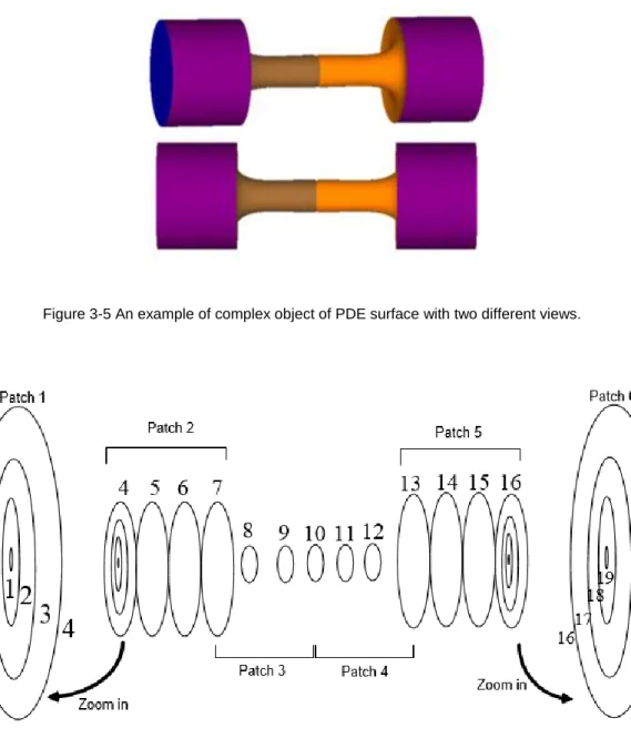
Figure 3-5 An example of complex object of PDE surface with two different
views. ... 40
ix
Figure 3-7 PDE face model taken from [46]. (a) represent 28 boundary curves
(b) the resulting PDE face ... 42
Figure 4-1 Example of 3D image taken from database ... 49
Figure 4-2 Example of face model taken from database. (a) two pod half-face image (b) face model with texture ... 50
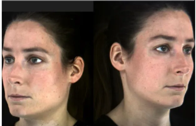
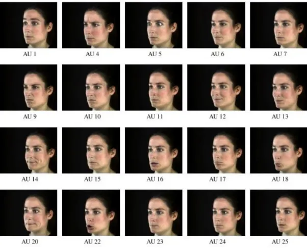
Figure 4-3 Images of Eva in 3D FACS database ... 51
Figure 4-4 Standardized and normalized face mesh ... 52
Figure 4-5 Feature points extracted from [96] ... 54
Figure 4-6 PDE face generated using 19 boundary curves, (a) randomly chosen points, and (b) uniformly chosen points ... 55
Figure 4-7 A neutral face and position of extracted curves,(a) generating boundary curves, (b) a face from the FACS database ... 56
Figure 4-8 PDE generated neutral face, (a) ten patches of continuous PDE surface (b) wireframe of full PDE face ... 58
Figure 4-9 Procedure for texturing PDE face, (a) two mesh overlapped together, where green mesh is PDE face (b) the closest mark with yellow vertices, and (c) PDE face with texture ... 60
Figure 4-10 Two meshes, PDE face (green mesh) and original face mesh overlapped to each other with three different cut-planes ... 62
Figure 4-11 Comparison of the accuracy between original mesh and PDE mesh for different cut-plane. ... 63
Figure 4-12 Flowchart shows methodology used for modelling PDE face ... 65
Figure 5-1 Some action units that relate to six basic expressions. This figure is reproduced from [99]. ... 67
x
Figure 5-3 Facial musculature (extracted from [16]) given in (a) is compared to
boundary curves in (b). ... 73
Figure 5-4 Facial feature points on Eva's face ... 75
Figure 5-5 Two meshes overlapped; neutral mesh and AU1 mesh ... 76
Figure 5-6 Boundary curves extraction process for AU1 (a) boundary curves from neutral face, (b) different mesh on forehead area of AU1 and (c) closest points indicated by yellow points ... 77
Figure 5-7 PDE generated facial action units (a) AU4 (b) AU12 (c) AU14 and (d) AU17 ... 79
Figure 5-8 PDE generated facial expressions (a) happy (b) sad (c) fear (d) disgust ... 80
Figure 5-9 Comparison of the accuracy between original mesh of AU4 and PDE mesh of AU4 for three different cut-planes. ... 82
Figure 5-10 Comparison of the accuracy between original mesh of disgust and PDE mesh of disgust expression for three different cut-planes... 83
Figure 5-11 Comparison of five different AUs using original mesh and generic PDE. ... 84
Figure 5-12 Flowchart shows methodology used for modelling and manipulating a PDE face ... 86
Figure 6-1 Overview of PDE face animation process ... 88
Figure 6-2 A portion of blendshape slider interface taken from [106] ... 90
Figure 6-3 Target face and base face ... 93
Figure 6-4 Varying weighting value for happy expression from (a) 0 (b) 0.229 (c) 0.534 (d) 1 ... 95
Figure 6-5 Blendshape sliders for fear, disgust and sad face expressions .... 96
xi
xii
List of Tables
Table 2-1 Upper face action units adapted from [57] ... 13
Table 2-2 Lower face action units taken from [57] ... 14
Table 2-3 Miscellaneous actions [57] ... 14
Table 5-1 AU combinations based on primary and auxilary AUs taken from [99]
... 68
Table 5-2 Expression description adapted from [101] ... 68
Table 5-3 Proposed AU combinations for facial expression ... 69
Table 5-4 Action unit related with facial expressions and their corresponding
facial muscles adapted from [51] and [57]. ... 71
Table 5-5 Action units and the corresponding boundary curves affected ... 74
xiii
List of Abbreviations
AU Action Unit
CAD Computer Aided Design
CAGD Computer Aided Geometric Design
CGI Computer Generated Imagery
FACS Facial Action Coding System
FAP Facial Animation Parameter
NURBS Non-uniform Rational B-Splines
xiv
List of Mathematical Symbols
, ( )
i m
B u Bernstein polynomial
, ( )
i m
N u B-Spline basis functions
,
i j
p Control points
( , )
X u v Parametric surface patch
,
m u v
D Partial differential operator of order m in independent
variables u and v
( , )
R u v Remainder function
( , )
1
1. Introduction
1.1 Background
Geometric models can be either in two-dimensional (2D) or three-dimensional
(3D) form. Geometric modelling includes both the definition of the geometry
and the development of the design method [1]. Computer Aided Design (CAD)
is the use of computer software and design for modelling the 3D virtual objects
[2]. Conventionally, surface design in CAD is based on polynomial
interpolation such as Bezier surfaces [3], B-Splines surface [4], and
non-uniform rational B-Splines (NURBS) surface [5]. Usually, these conventional
surface generation techniques use a polynomial based method and the
surface is generated using a set of control points. In order to change the shape
of the objects, the designer needs to manipulate the control points to get the
desired shape. This conventional method has the disadvantage of being time
consuming: complex objects are usually represented by a large number of
control points and consequently, it is difficult to manipulate underlying
geometry in a timely manner [6].
In order to overcome this limitation, Bloor and Wilson [7] introduced the
Partial Differential Equations (PDE) method. Their pioneering work was firstly
used for blending surfaces and the generation of free-form surfaces [8]. The
PDE method regards the generated surfaces as the solution of
boundary-value problems. More precisely, the PDE method considers a surface as the
graphical representation of the solution to elliptical partial differential
2
results in smooth surfaces along the boundaries and at the same time,
satisfies the continuity conditions of blend shapes. The PDE method gives
flexibility to manipulate the object shape as it is based on boundary conditions
imposed on each particular case.
The human face is a complex 3D geometric form [9] and is very flexible
[10]. These characteristics make human facial modelling very challenging in
computer graphics. Facial modelling is a technique for representing the face
on a computer [11] and more attention is given to modelling 3D human faces
as a 3D face model has the robust features of a human face [12]. It is hard to
model a geometry with no rigid structure [10].
Facial expressions are important for communication between people in
order to convey their emotional state [13]. Humans are special as they can
understand other people’s facial expressions by understanding a message communicated verbally or by nonverbal communication [14]. As humans
become heavily dependent on computers, it will be useful if computers can
synthesis human facial expressions in order to improve human-computer
interaction [15].
In order to form a desired facial expression using a computer, there are
many methods that can be used for describing the muscle movement on a
human face. Two popular methods are MPEG-4 facial animation standard [16]
and facial action coding system (FACS) [17]. MPEG-4 standard used the
Facial Animation Parameters (FAP) coding system to defines facial motions
by creating displacement on a predefined location on a face with respect to
3
units [17]. An action unit (AU) represents the simplest visible facial movement,
which cannot be decomposed into more basic ones [17].
Facial animation is a branch in computer-generated imagery (CGI) and
studies a way to design virtual faces for creating human-like facial expressions
[19]. Animating a human face is a complex task that requires modelling and
animating the motion of facial movement [20]. Facial expression animation is
one of the challenging tasks in computer graphics as facial expressions are
very complex and they are paramount in nonverbal communication channels
[21].
3D face models are useful in extensive applications such as automatic
facial recognition [22], facial animation [23], human-computer interaction ([24],
[25]), avatar [26] and etc. In most application scenarios, human face modelling
and animation get extra attention in computer graphics due to the diversity and
complexity of facial expressions [27]. Advanced development of computer
facial animation technique was driven by significant requirements in the
entertainment industry such as films and video games, where face and facial
expressions are important to describe the emotions of an animated character
[28]. In communication applications, the interactive talking faces make
human-computer interaction superior by providing a friendly interface [29].
1.2 Motivation
Generating realistic facial animation often involves complex modelling
techniques based the structure of the facial model for determining its animation
4
choose either to build multiple face layers [31] or to carry out deformation on
the face models [32]. Hence, the quality of facial animation is determined by
both the employed methods of facial modelling and facial animation [33]. Since
the pioneering work by Parke [10], significant research effort has been
attempted for modelling the geometry of human faces including blendshapes,
direct parameterisations and muscle based modelling [16].
Blendshape models provides a compressed representation of the facial
expressions by specifying the blendshape weight [34]. Facial motion can be
represented by varying the weights of linear combinations [35]. Blendshape
technique is one of the popular facial animation due to its efficiency and
intuitive controllability [36]. However, modelling a complex facial expression
using a blendshape model is very time consuming and needs a lot of storage
for large libraries of blendshapes [37].
Parametric models offer an alternative approach to a blendshape model
as a parameterised face can be manipulated directly by changing a few
corresponding parameters [38]. A parameterisation technique can divide a
face into different small parts in order to give animators more control over facial
configurations [39]. Most parametric models employ MPEG-4 Facial Animation
Parameters [40] or FACS [41] for describing facial expressions. In contrast, it
is hard to determine suitable parameters for controlling facial expressions of a
parametric model [16] and manual tuning is required when adapting a new
facial model to the existing parameterised model [42].
A muscle based model is a polygonal surface mesh that is constructed
5
the physical properties of the facial muscles and articulations [43]. Muscle
based method produces a realistic 3D animation by precisely simulating the
facial muscular tissue contraction for representing facial expressions [16].
Furthermore, facial expressions in a muscle based model are controlled by a
set of parameters that are related to action units for describing muscle
movement [17]. The muscle model is broadly used due to its compact
representation and is not dependent on facial mesh structure [39]. Although,
a muscle based model can generate a realistic face model, the modelling
process of an anatomical facial structure is an extremely tedious task, which
needs massive computation of the underlying structure and requires artistic
skill to place the muscle points correctly to the face model [44].
Based on the three facial models mentioned above, it is concluded that
the modelling of a human face needs further improvement in terms of
representation of facial data, storage capacity for storing facial information and
a well-defined set of control parameters for easy manipulation in order to save
time. The researchers still need to find a more sophisticated technique for
representing a 3D human face in an accurate and efficient way [45] and at the
same time the face geometry can be manipulated easily [21]. The face model
should also be compatible with animation systems to avoid a new face needing
to be modelled for each time frame [32].
Thus, the research goal of this work addresses the above limitations in
a previous 3D face model using a boundary value approach, to be exact, the
PDE method. With the rapid development of computer graphics, the PDE
based geometry modelling technique has recently been considered as a
6
such as Bezier, B-Spline and NURBS [46]. The PDE-based face is considered
a powerful tool to describe face geometry because a very small parameter is
needed to specify and generate a specific face with a specific expression that
is produced with low cost [47]. Furthermore, integrating FACS on boundary
curves in the PDE method would be advantageous as these boundaries play
a significant role in facial modelling.
1.3 Objectives
The aim of this research is to develop a mathematical formulation based on a
boundary-value problem for representing an action unit for a human face. In
particular, muscle movement of action units is formulated as the solution to
elliptical partial differential equations. This research will explore a technique
using PDE based formulation to represent and model action units. A
PDE-based face has some benefits such as efficient storage of facial data, smooth
PDE surface with associated FACS based muscle movement, efficient
manipulation of facial geometry and time saving when animating facial
expressions.
The objectives of this research are summarized as follows:
i. To utilize PDE based formulation for generating a smooth human face
in 3D space and apply a simple texturing method on PDE face for a
realistic looking face.
ii. To exploit the formulation of the PDE method by representing facial
muscle movement on human faces using a small number of control
7
iii. To generate various action units of a human face based on the use of
PDE method by using a different PDE descriptor.
iv. To explore different combinations of PDE descriptors for generating
basic facial expressions of a human face.
v. To apply the formulation of PDE descriptors in one of the simple
animation technique by animating the facial expressions of PDE-based
face.
1.4 Research contributions
This thesis offers the following contributions:
i. The PDE-based face adopted in the work is achieved by mapping the
boundary curves with key features of the face to generate a smooth
face surface (Chapter 4).
ii. Simple texturing method for realistic looking models (Chapter 4).
iii. PDE descriptors that are used for representing different action units will
reduce the storage capacity for storing the facial data (Chapter 5).
iv. Generated PDE-based face of different facial expression by combining
different action units is an effective way for manipulating a PDE face
from a neutral configuration to an expressive face (Chapter 5).
v. Animation of four different basic expressions using a generic PDE face
will save a lot of time as a generic model can be used without manual
8
1.5 Publications
The list of publication of the works in this thesis are listed as follows:
1. H. Ugail and N.B. Ismail, “Method of Modelling Facial Action Units using
Partial Differential Equations”, in Advances in Face detection and Facial Image Analysis (Springer, 2015), To Appear. (2015).
2. N. B. Ismail and H. Ugail, “Modelling of Facial Expressions using Partial Differential Equations”, Under preparation, to be submitted to The Visual Computer (2015).
3. N. B. Ismail and H. Ugail, “Blendshape Based Facial Animation using
Partial Differential Equations”, Under preparation, to be submitted to The Visual Computer (2015).
1.6 Structure of the thesis
The rest of the thesis is structured as follows:
Chapter 2, “Face model and animation”, gives an introduction to the
FACS and facial animation. The first section provides some details on
action units including both parts of FACS classification; upper face
action units and lower face action units. The second section examines
various animation techniques based on geometric facial animation,
which includes key framing and blendshapes interpolation, direct
parameterization and muscle based animation. Some literature of
9
Chapter 3, “Geometric modelling of surfaces and human faces”,
presents the literature of surface generation including the conventional
method in CAD and the proposed method, PDE method. More
discussion focuses on the PDE method as it is the main approach of
this work. The last part of this chapter gives some literature of work that
has been done in modelling human faces using PDE surface
generation.
Chapter 4, “PDE-based facial modelling”, offers detail on the
methodology of PDE face parameterisation. There are five procedures
involved for parameterisation of PDE face: selecting 3D mesh from
database, pre-processing, extracting boundary curves, solving elliptic
PDE equation and texturing.
Chapter 5, “PDE-based facial expression”, presents a methodology
for manipulating a generic PDE face of neutral expression to a face with
an expression. This chapter will demonstrate a technique to formulate
a method to store the action units known as PDE descriptors.
Manipulation of a generic PDE face from a neutral PDE-based face to
a given action unit also will be explained in this chapter. Furthermore,
this chapter also will be described a method for generating an
expressive PDE-based face models by combining related PDE
descriptors that results of generation of four different basic expressions
namely happy, sad, fear and disgust.
Chapter 6, “Animation of PDE-based face”, presents a technique
10
expressions by using the generic PDE face. The result is given
graphically as animation sequences.
Chapter 7, “Conclusions”, concludes the overall research that has
been done. This chapter will summarise the research that has been
done, state the contributions, give the research limitations and suggest
11
2. Facial animation
2.1 Introduction
Facial modelling can be grouped into two different approaches namely
based facial modelling and geometric-based facial modelling [48]. In
image-based facial modelling, the creation of a facial model is image-based on a collection
of facial images captured from a real person’s face [49]. In contrast, geometric-based facial modelling refers to generation and manipulation of geometry
representation of 3D face models [11]. In geometric modelling, the detailed
data for representing geometry of facial data can be obtained by photographic
techniques, 3D digitizers, or 3D laser-based scan [17]. The approach used in
this work is based on geometric modelling.
In this chapter, the related research papers is discussed. The first
section provides some details on the Facial Action Coding System (FACS), as
FACS is used to describe muscle facial movement. Then it is followed by a
summary on the state of the art 3D facial animation that focuses on a
geometric-based technique. Later, some literature of animation techniques
based on FACS is given.
2.2 The Facial Action Coding System (FACS)
FACS was originally developed by a group of physiologists, Paul Ekman,
Wallace Friesen and Joseph Hager, in the 1970s [50]. Since then, FACS has
12
behaviour ([51], [52]). Facial behaviour is determined by measuring the stretch
of facial muscles that affects the changes on the appearance of the face ([53],
[54]). The measurement unit of FACS is called an Action Unit (AU). For
example, AU1 is inner brow raiser, AU4 is brow lower, etc. There are 44
different action units defined by FACS, each of which corresponds to a given
activity in a distinct muscle or group and produces characteristic facial
distortions [55].
FACS is classifies action units into two main groups: upper face action
units and lower face action units. These action units are based on muscle
movement [24] and the type of muscle [56]. In fact, the muscle can be
categorised according to the fasciculi (the individual fibers of the muscles) that
may be parallel, linear, oblique, or spiralled relative to the direction of pull
where it is attached [57]. The main muscles on a human face, according to
Waters [31], are shown in Figure 2-1.
13
Based on Figure 2-1, the upper facial muscles are responsible for changing
the appearance of the eyebrows, forehead, and upper and lower lids of the
eyes [31]. The related contraction of a specific of upper face facial muscles is
adapted from [57] is shown in Table 2-1.
Table 2-1 Upper face action units adapted from [57] AU Number FACS name Facial muscle
1 Inner brow raiser Frontalis, Pars Medialis 2 Outer brow raiser Frontalis, Pars Medialis
4 Brow lowerer Depressor Glabella, Depressor Supercilli, Corrugator
5 Upper lid raiser Levator Palpebrae Superioris 6 Cheek raiser Orbicularis Oculi, Pars Orbitalis 7 Lid tightener Orbicularis Oculi, Pars Palebralis
On the other hand, the lower face action units, are classified in five major
groupings as follows [31]:
Up/down actions; they move the face upwards towards the brow and conversely towards the chin, i.e. AU9 for nose wrinkler.
Horizontal actions; the muscles that contract horizontally towards the ears and conversely towards the centre line of the face, i.e. AU14 or
known as dimpler.
Oblique actions; they contract in an angular direction from the lips, upwards, and outwards to the cheekbones, i.e AU12 for lip corner
puller.
Orbital actions; they are circular or elliptical in nature, and run round the eyes and mouth, i.e. AU18 for lip pucker.
Sheet muscles; carries out miscellaneous actions, particularly over the temporal zones and platysma muscle, i.e. AU19 (tongue show) and
14
The full list of lower facial action units taken based on [57] are described in the
Table 2-2.
Table 2-2 Lower face action units taken from [57]
AU Number FACS name Facial musle
9 Nose wrinkle Levator Labii Superioris, Alaeque Nasi 10 Upper lip raiser Levator Labii Superioris, Caput Infraorbitalis 11 Nasalobial furrow
deepener
Zygomatic Minor 12 Lip corner puller Zygomatic Minor 13 Sharp lip corner Caninus
14 Dimpler Buccinator
15 Lip corner depressor Triangularis 16 Lower lip depressor Depressor labii
17 Chin raiser Mentalis
18 Lip puckerer Incisivii Labii Superiorsis, Incisivii Labii Inferioris
20 Lip stretcher Risorious
22 Lip funneler Orbicularis Oris 23 Lip tightener Orbicularis Oris
24 Lip pressor Orbicularis Oris
25 Lips part Depressor Labii, or Relaxation of Mentalis or Orbicularis Oris
26 Jaw drop Massetter, Temporal and Internal Pterygoid Relaxed
27 Mouth Stretch Pterygoid, Digastric
28 Lip suck Orbicularis Oris
41 Lip Droop Relaxation of Levator Palpebrae Superiosis
42 Slit Orbicularis Oris
43 Eyes closed Relaxation of Levator Palpebrae Superiosis
44 Squint Orbicularis Oris
45 Blink Relaxation of Levator Palpebrae and
Contraction of Orbicularis Oris, Pars Palpebralis
46 Wink Orbicularis Oris
In total, there are 30 AUs that anatomically relate to a contraction of a specific
set of facial muscles (as listed in Table 2-1and Table 2-2). Another 14 AUs,
are known as miscellaneous AUs that is shown in Table 2-3. They are not
based on their muscular basis and their specific behaviour is not entirely
distinguished [31].
Table 2-3 Miscellaneous actions [57] AU Number Description
8 Lips towards 19 Tongue show 21 Neck tighten 29 Jaw trust
15 30 Jaw sideways 31 Jaw clench 32 Bite lip 33 Blow 34 Puff 35 Cheek suck 36 Tongue bludge 37 Lip wipe 38 Nostril dilate 39 Nostril compress
An additional feature of FACS is that of scoring measurements for the intensity
with which action units are performed. These scores are scaled from A to E.
Figure 2-2 shows the relationship of intensity scores and scale of evidence
[50].
Figure 2-2 Relation between the scale of evidence and intensity scores taken from [50]
The terms A, B, C, D and E in Figure 2-2 respectively describe the intensity as
classified from visible to maximum intensity of each AU [50]. However, the
work in this thesis only considers the highest intensity of selected action units
when modelling each action unit. For instance, the AU4E indicates AU4 with
an intensity of E, which means that the brow was pulled together or lowered
with maximum intensity.
2.3 Geometry based facial animation
This section will survey facial animation techniques that are based on facial
geometry. Geometry based facial modelling and animation techniques include
16
muscle based animation ([58],[42]). For a full survey of facial animation
method, a book by [30] can be referred to as it has reviewed all the complete
techniques for facial animation.
2.3.1 Key framing and blendshape interpolation
A key-framing method with interpolation is by far the simplest and oldest
approach [11], but still frequently used by animators because of its intuitive
and flexible controls [59]. In fact, the pioneer work for facial animation
demonstrated the use of this approach by Parke [10]. In particular, Parke
describes a facial geometry in at least two different expressions and uses
linear interpolation for manipulating the face from one expression to the other
[43]. He used relatively small numbers of polygons to represent the face (as
shown in Figure 2-3) and explicitly key framed the data of animation [11]. Even
using a small number of parameters, Parke’s face model can be rendered smoothly and facial features (eyes, nostrils, teeth, eyelashes and eyebrows)
were added for a realistic head model as illustrated in Figure 2-3. However,
this approach is not practical for complex facial expressions and needs a lot
of storage to store the animation data [60].
Figure 2-3 Parke’s face model of the same person in different shading, left was rendered using polygonal shading and right was rendered using Gouraud’s smooth shading. The images were taken
17
Although more sophisticated animation techniques have been
developed to date, key-framing and blendshape interpolation remain popular
among animators and are commonly used in commercial animation software
packages such as Maya and Studio Max [35]. More discussion on
blendshapes will be covered in Chapter 6.
2.3.2 Direct parameterisation
In order to overcome the limitations of key framing and blendshapes, Parke
derived a method called direct parameterisation [38], where facial expressions
can be generated and manipulated by specifying appropriate sets of
parameters [61]. The facial expressions are represented by a small parameter
even when the face is represented using polygonal surface [11]. Thus, a wide
range of facial expressions can be animated by combining related parameters
with a relatively low cost of computation [62].
There are some limitations inherited from a direct parameterisation
animation technique. This animation technique is not suitable for a complex
facial model that consequently produces a very large number of vertices [42].
The choice of the parameters set depends on the facial topology, it is
impossible to generate a complete set of facial expressions [48]. Thus, this
limitation will lead to unnatural expressions especially when manipulating a
vertex that is represented by the same parameter [63]. Furthermore, a new
face model requires a manual manipulation task in order to adapt the generic
face to an existing parameterisation animation scheme [42].
However, the work by Sheng et al [47] eliminated some limitations
18
the PDE method can produce and animate a 3D face using a small number of
parameters. They successfully animated six facial expressions as given in
Figure 2-4.
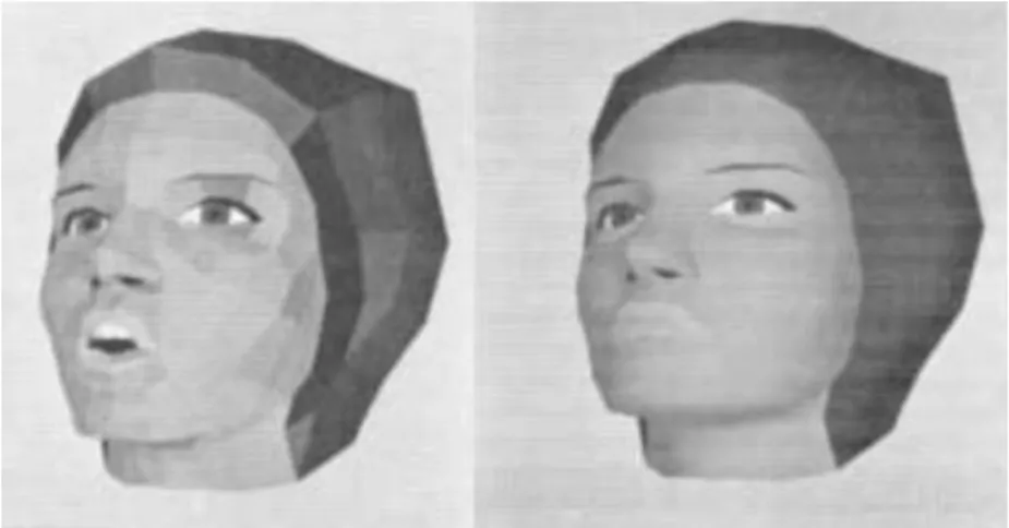
Figure 2-4 PDE face with six facial expression namely (from left to right) joy, sadness, anger, fear, disgust and surprise. The face of expressions were taken from [47].
The facial animation above uses a direct parameterisation scheme by
associating PDE boundary curves with MPEG-4 Facial Animation Parameters
(FAPs).
2.3.3 Muscle based animation
A muscle based approach simulates real human face muscles for animation
purposes [63]. The earliest approach towards a muscle based model was
proposed by Platt and Badler [64], where animation was applied by a set of
facial action units using a contraction algorithm. They constructed an abstract
muscle fibre structure that was connected by spring for connection of skin,
muscles and bone nodes in their system [65]. Later, Water [31] presented an
animation of a human face that used FACS for describing the muscle
movement and representing facial expression. Water’s muscle models as shown in Figure 2-5 are the basis principle of widely used physic-based
19
Figure 2-5 Water's facial muscles distribution taken from [39]
The physic-based model approach is divided into three categories [48]:
mass spring systems. These spring systems are applied on a face to
force simulation of skin deformation.
layered spring meshes. They extend mass spring muscles into three
connected mesh layers for realistic facial behaviour.
vector muscles. They define a vector field as muscle for contraction of
mesh vertex.
Among these three approaches, a vector muscles model uses FACS for
animating human emotions such as anger, fear, surprise, joy and happiness
by using orbicularis oris muscles and linear muscles (blue line in Figure 2-5).
The facial expression that was generated by Waters work [31] is given in
20
Figure 2-6 Facial expressions generated by Water’s namely neutral, happy, anger, fear, surprise and disgust (from left to right). All facial expressions are extracted from [31].
Animation of facial expression in Figure 2-6 is achieved by changing the
contraction of muscle parameters, where these parameters are embedded
under the face mesh with an assumption that the muscles are placed correctly
under the face mesh [66]. However, finding correct positions to anatomically
locate the position of vector muscles is a daunting task [48] as it is not intuitive
or consistent from one model to another face model.
2.4 FACS-based animation
Based on animation techniques discussed in the previous section, there exists
some facial models that utilized FACS as a basis for control parameters as
shown in [64] and [31]. To be exact, muscle based animation employs action
units in the face models for animating facial expression by changing the
relevant parameters. Since then, more research has adopted FACS in the face
model for generating realistic facial animation. This section will review some
of related works that employ FACS as parameter controls in facial animation.
The work in [61] introduced an anatomically-based arrangement of
muscle model, along with a physically-based tissue model. The tissue model
is developed by considering the biomedical of tissue mechanics for more
21
model that was introduced in [31] through FACS abstraction in order to provide
a more convenient interface to the face model for representing facial
expressions. This physical-based tissue model contains a total of 960
polygons with approximately 6500 spring units. Hence, a lot of storage is
needed to store the face data and it needs a high speed computer for
simulation of facial expressions.
Later, a face model based on non-linear spring frames is proposed in
[44], that can simulate the dynamic of real skin. This 3D physical based model
is also based on human facial anatomy and has the 3D structure of muscle
and skin. Facial muscles are modelled as forces for deforming the spring
mesh. They use ten major functional facial muscles from [31] which is based
on FACS and simulates the muscle contraction for generating a facial
expression. By determining the facial muscles parameters, this non-linear face
model can analyse the relationship between the facial skin deformation and
inside the mesh face. In contrast, this work also inherits the same problems as
previous work in [61], which it also requires a big amount of storage.
A 3D model of a specific person is presented in [37] for producing
natural looking animations where facial geometry is reconstructed individually
from a laser scan range. Three kind of facial muscle models are developed for
simulating facial muscle contraction. They do not use all 46 AUs in FACS but
simplify the model by selecting 18 action units that strongly influence the facial
expression. Facial expression is parameterised by FACS, where a simple
linear combination of action units approximates the muscle contraction.
However, simulation of facial expression of such a model increases computing
22
All facial models discussed above use Water’s muscle model as shown in Figure 2-5. It is shown that using FACS in a muscle based model, the facial
expression can be animated by combining one or more action units. Instead
of using muscle-based modelling, the work in this thesis will adopt Water’s muscle model to a parametric surface in order to overcome the problems with
storage capacity and computing time. For this purpose, parameterisation of a
human face will use the PDE method, by embedding Water’s muscle model to the boundary curves. More discussion on the PDE method will be presented
in Chapter 3. Then in Chapter 4, a detailed methodology of PDE face
parameterisation is given. However, the goal of this work is not to develop a
highly realistic looking facial model, but a model that would be able to be
realistic in a natural way.
2.5 Summary
In this chapter, the discussion begins with a detailed explanation about FACS,
which includes both FACS classifications; upper face action units and lower
face action units. Facial muscles corresponding to each action unit are also
given for both categories as a reference of Chapter 5. A knowledge of muscle
distribution is needed when extracting boundary curves for representing the
action units.
The second section of this chapter has examined three different
techniques of geometry facial modelling and animation: key-framing and
blendshapes interpolation, direct parameterisation and muscle based
23
modelling is based on anatomy and a physics based model successfully
represents a realistic facial animation of expressions based on FACS. This is
supported by some literatures] given in the last section.
Thus, the approach that has been used in this research is an integrated
approach of all three techniques discussed above. In particular, our method
adapted muscle movement from the model-based approach by Waters [31]
when locating the facial features that are related to FACS. Then, a face model
is parameterised using the PDE method as the PDE method only stores a
small amount of parameters for representing the face and can be manipulated
by changing the related parameters. For animation purposes, this work will
employ key-framing and blendshape interpolation as it is the simplest
24
3. Conventional methods of surface modelling and
PDE-based face modelling
3.1 Introduction
In the previous chapter, various animation techniques in geometric modelling
have been discussed including key-framing and blend shape animation, direct
parameterization and muscle-based animation. The goal of these animation
techniques is to control the geometry of the face until the rendered facial
geometry has the desired expressions and textures in each frame of the
animated sequence [30]. Furthermore, the face model that is used in the
modelling stage will determine the animation potential [42]. Hence, the correct
choice for a facial modelling method is important so that the face model can
be easily manipulated for desired expressions and animated in realistic
movement.
After reviewing different approaches for facial animation, blend shapes
interpolation suits the nature of this research considering its popularity,
efficiency, and intuitive controllability. Here popularity refers to a highly
preferred method by the animator [67], as blend shapes are a standard
component of commercial animation packages such as Maya and Softimage
[68]. However, a traditional blend shapes method which is based on polygonal
models has disadvantages when animating desired animation due to tedious
and labouring work [67] for correcting vertex positions manually. Considering
this disadvantage, some works used parametric models for more intuitive
25
used a NURBS face model composed of 46 blend shapes while Li and Deng
[69] used spline base curves for smooth animation.
In this thesis, a face model is based on a parametric surface, to the
exact PDE parametric surface. The purpose of this chapter is to review various
modelling techniques that have been used in computer graphics for generating
parametric surfaces. It begins with a general discussion about conventional
method for generating parametric surface including Bezier, B-Spline and
NURBS. Then, the mathematical concepts of PDE method for surface
generation are discussed in detail as the PDE method is the main approach of
this research. Later, an overview of previous approaches for modelling faces
using PDE surface generation is given.
3.2 Conventional methods of surface representation
In geometric modelling, a variety of surfaces are used by researchers for
representing surfaces. The most common methods are implicit equations and
parametric functions.
The implicit surface is represented in general form as f x y x( , , )C in
3D-space. Note that x, y and z are Cartesian coordinates and C takes any
constant. If the equation is linear and it is given by ax by cz 0, then it is a plane. If the equation is in second order of a quadratic surface, the equation
being 2 2 2 2
x y z r , then it represents a surface of sphere. These two
examples of equations are implicit because one can test directly either if any
26
then it is concluded that the points lay on the surface. The implicit surface is
rendered using various techniques such as polygonization, ray-tracing and
contours [70].
A parametric surface is more popular and known as polynomial based
method. This polynomial based method can be used to generate complex
geometries that are defined by a set of control points. The popularity of
parametric surface representation is due to the fact that they can be easily
manipulated. The work in this thesis used parametric surfaces for face
modelling. Thus, a detailed discussion of a parametric surface is outlined in
the next subsection consisting of various methods of conventional surface.
These conventional methods refer to Bezier surface, B-Spline surface, and
NURBS surface. At the end of this chapter, an alternative method to
conventional surface that is known as PDE based surface generation is
presented.
3.3.1 Parametric surface
Parametric surface representation consists of mapping two parameters
u and w, into three function xx u w y( , ), y u w( , ) and zz u w( , ). In general, a parametric surface takes the form:
( , ) ( , ) ( , ) ( , ) x u w X u w y u w z u w . (3.1)
It is basically a mapping of a domain 2
R
to 3
R . Figure 3-1 (extracted from
[71]) shows an example of a parametric patch. Some of the most popular
27
surfaces and Non-uniform rational B-Spline (NURBS), which are discussed in
detail in the following section.
Figure 3-1 Parametric surface patch taken from [71].
3.2.2 Bezier surface
A Bezier surface is defined by a two-dimensional set of control vertices and
Bernstein polynomial basis function [72]. If the Bezier surface of order (m n )
is denoted by X u w( , ), then the equation of Bezier surface is given by
, , , 0 0 ( , ) ( ) ( ) m n i m j n i j i j X u w p B u B w
(3.2) where pi j, denotes the control points. pi j, are the vertices of control polygon that form an (m1) by (n1) .
B
i m,( )
u
is a Bernstein polynomial in u-direction. The Bernstein polynomial is defined explicitly byBi m, ( )u m ui(1 u)m i i (3.3)
28
where the binomial coefficients are given by
! ; 0 !( )! 0 ; m i m m i m i i otherwise (3.4)
Similarly,
B
j n,( )
w
is Bernstein polynomial in w-direction.These Bernstein polynomials,
B
i m,( )
u
andB
j n,( )
w
, are also known as Bezier basis function. The Bezier basis functions are non-negative over the interval(0,1) and their summation in interval (0,1) is one ( ,
0 ( ) 1 m i m i B u
and , 0 ( ) 1 n j n j B w
).Bezier surfaces possess convex hull property, which means the surface
remains within the convex hull of control points. Bezier surface also offers an
intuitive way of creating and manipulating a generated surface by manipulating
the control points [71]. However, the object represented with a massive
number of control points tends to be impractical, time consuming and would
require a vast amount of storage space [73].
Another drawback of Bezier surface is that their control points have
global control. Global control means the adjustment of a small set of control
points have global control. Global control means the adjustment of small set
of control points will affect the overall shape of the object. The problem occurs
when one cannot make minor adjustments to create a desired shape. Local
29
a certain surface. The local control techniques include B-Spline and NURBS
surfaces [74].
3.2.3 B-Spline surface
B-Spline surfaces play an important role in geometric modelling.
Mathematically, a Spline surface is a product of control vertices and
B-Spline basis function that can be written as follows
. , , 0 0 ( , ) ( ) ( ) m n i j i m j n i j X u w p N u N w
. (3.5)It is assumed that one knot sequence is in the
u
-direction and one in thev
-direction. The term
N
i m,( )
u
is a B-Spline basis functions that is given by1 , , 1 , 1 1 1 ( ) i ( ) i m ( ) i m i m i m m i m i i m i u u u u N u N u N u u u u u (3.6) where 1 ,0 1 ; ( ) 0 ; i i i u u u N u otherwise (3.7)
The term
N
i m,( )
u
in Equation (3.6) is called a normalized B-Spline of degreem. The interval
u ui, i1
is called the i-th knot span and the knot vector is defined as U
u u0, 1, ,um
.In geometric design, there are two types of knots which are used;
uniform (with equally spaced knots) and non-uniform. In addition, if the first
and the last knots are repeated
m1
times then the knot vector is non-uniform and non-periodic. Non-non-uniform knot vectors provide great flexibility for30
various design applications [74] and give the advantage of manipulating only
a small part of the surface accordingly.
The main difference between B-Spline and Bezier surfaces is that in the
case of Bezier surfaces, the control polygon uniquely defines the surface,
whereas B-Spline surface requires the knot vector in addition to the control
polygon. This property of B-Spline is called knot insertion. By adding extra
knots to the control polygon, the approximation of the generated surface is
greatly improved. Therefore, by adding more knots, one can easily limit the
area affected by a control point modification otherwise known as local
modification of the surface [73].
3.2.4 NURBS surface
The most popular surface in geometric modelling is NURBS surface. It offers
a common mathematical form for representing and designing free form
surfaces. NURBS curves represent a natural generalization of B-Spline and
Bezier curves. Bivariate NURBS surfaces are the proper generalization of
tensor product B-Spline and Bezier surfaces [74].
Extending the formulation of B-Spline in ( , )u v space, the formulation of
NURBS is given by:
, , , , 0 0 , , , 0 0 ( ) ( ) ( , ) ( ) ( ) n m i j i j i p j q i j n m i j i p j q i j p N u N v X u v N u N v
(3.8) where31
pi j, forms a control polygon. The control polygon is defined over the
knot vectors as follows:
U
u u1, 2, ,un p 1
(3.9)V
v v1, 2, ,vm q 1
(3.10)
N
i p, andN
j q, are normalized B-Splines of degree p and q respectivelyin the u and v directions. Normally, u
0,1 and the surface isundefined outside the domain.
NURBS surfaces are useful because they are invariant under rotation, scaling,
translation and perspective transformation of the control points [2]. The most
useful properties of NURBS surface is localness where one can manipulate
the NURBS surface by repositioning the control points or altering the value of
surface weight [75]. This characteristic gives NURBS surface a flexible way to
design a large variety of shapes. However, the NURBS surface needs a lot of
control points to define a complex surface such as a human face, thus it
requires a bigger storage capacity. This disadvantage is not particular to
NURBS. Other polynomial based surface generations also exhibit the same
problem.
3.3 PDE surfaces
Given that conventional methods need huge amounts of storage to define
complex geometry, Bloor and Wilson have introduced a PDE method, which
32
boundary conditions to generate any given object. The PDE method is able to
parameterize complex surfaces using a small set of design parameters
compared to conventional methods, which require hundreds of control points.
The PDE-based method was primarily introduced in surface blending
[7] and followed by free-form surfaces [8]. In recent years, the PDE-based
method has widened its application to graphics and modelling including;
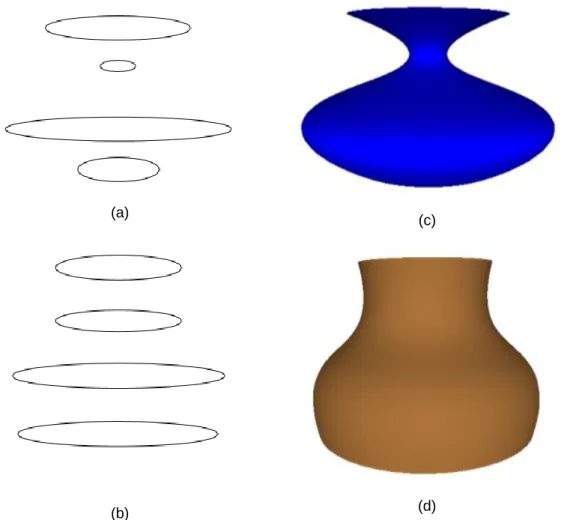
modelling of wing geometries [76], interactive design [77], vase design [78],
aircraft geometry [6], pharmaceutical tablets [79], among others.
3.3.1 PDE surface patches
The PDE method produces parametric surface patches, X u v( , ), defined by
two parameters, u and v, in finite region 2
R
with a specified boundary,
. Here X u v( , ) is regarded as a mapping point in to a point in Cartesian space such that
R
2( )
E
3. In order to find X u v( , ), it is required to find a solution to the partial differential equation given by:, ( ) ( , ) m u v D X F u v (3.11) where m, u v
D is a partial differential operator of order m in independent
variables u and v.
F is a vector-valued function of u and v.
The function F is included for completeness and usually the value is zero [80].
Usually, the choice of the operator ,
m u v
33
smooth surfaces for boundary-value problems. The choice of order m
depends on the level of surface control and continuity required for the shape
of the surface. If a second order PDE is used, there are no tangential boundary
conditions therefore the designer loses the ability for controlling the shape of
the surface. In general, the more flexible and powerful surface is archived by
higher order PDE [81]. For this research, the fourth-order PDE is used, where
four boundary conditions are needed for each X u v( , ) patch.
The general form of a fourth-order elliptic PDE over 2D parametric
domain is given by:
2 2 2 2 2 a 2 X u v( , ) 0 u v . (3.12) where
X u v( , ) is a PDE surface in a domain . The boundary conditions are
imposed on the functions X u v( , ) and its normal derivatives (Xu and
u
X ) at the edge of the surface patch.
a is a smoothing parameter and a0. This special design parameter
controls the relative smoothing of the surface in the u and v directions.
Note that Equation (3.12) is known as Biharmonic equation if a1. The
Biharmonic equation can model some phenomena related to solid and fluid
mechanics. It is also useful in engineering analysis that relates with
stress/strain analysis problems. Hence, there are different methods that have
been developed for solving Equation (3.12) ranging from analytical solution
34 3.3.2 Solution to the PDE method
As mentioned above, there are various techniques that can be used to find the
solution of Equation (3.12). The work described in this thesis is based on
spectral approximation [83] where the approximation solution of the PDE
surfaces is calculated using Fourier analysis and gives the solution in closed
form including a remainder term.
Equation (3.12) is solved over the region of a parameter plane, subject to a set of boundary conditions on the solution X , Xu and Xv around
the boundaries of specified region, where 0 u 1 and 0 v 2
. Boundaryconditions on X are imposed for defining the shape of the trim lines in physical
space in terms of u and v, and the first derivative continuity, Xu and Xv, is
required for specifying the surface normal
XuXv
along the trim lines.The boundary conditions that are used to solve Equation (3.12) are
specified as follows: 0 (0, ) ( ) X v P v (3.13) 1 (1, ) ( ) X v P v (3.14) 0 (0, ) ( ) u X v d v (3.15) 1 (1, ) ( ) u X v d v (3.16)
Note that P v0( ) defines the edge of the surface patch with derivative
conditions d v0( ) at u0 and P v1( ) defines the edge of the surface patch with
35
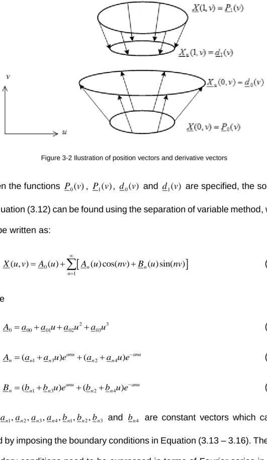
Figure 3-2 Ilustration of position vectors and derivative vectors
When the functions P v0( ), P v1( ), d v0( ) and d v1( ) are specified, the solution
of Equation (3.12) can be found using the separation of variable method, which
can be written as:
0 1 ( , ) ( ) n( ) cos( ) n( ) sin( ) n X u v A u A u nv B u nv
(3.17) where 2 3 0 00 01 02 03 A a a ua u a u (3.18) 1 3 2 4 ( ) anu ( ) anu n n n n n A a a u e a a u e (3.19) 1 3 2 4 ( ) anu ( ) anu n n n n n B b b u e b b u e (3.20)and an1,an2,an3,an4,bn1,bn2,bn3 and bn4 are constant vectors which can be
found by imposing the boundary conditions in Equation (3.13 – 3.16). Then the boundary conditions need to be expressed in terms of Fourier series in order
36
0( )
d v and d v1( ) can be expressed in terms of finite Fourier series, the solution
to Equation (3.17) is also finite.
However, when the functions at boundaries cannot be expressed in
terms of finite Fourier mode, therefore, the solution is infinite. In this case, an
approximate technique is often used and is based on the sum of the first few
Fourier modes and a remainder term as follows:
0 1 ( , ) ( ) ( ) cos( ) ( ) sin( ) ( , ) N n n n X u v A u A u nv B u nv R u v
(3.21)where N is finite (usually N5 ) and R u v( , ) is a remainder function. The coefficient functions A un( ) and B un( ) are given by Equation (3.19) and (3.20),
which can be determined from the amplitudes of the first N Fourier modes in
boundary conditions. For example, a Fourier analysis of the boundary
conditions allow P0 to be written as:
0 0 1 ( ) cos( ) sin( ) . N n n n P v a a nv b nv
(3.22)The remainder function R u v( , ) represents the contribution of high frequency
mode where it can be written as
1 2
3 4
( , ) ( ) ( ) u ( ) ( ) u
R u v r v r v u e r v r v u e (3.23)
and the r r1, 2,r3 and r4 are obtained from the Fourier analysis by considering
the difference between the original boundary conditions and the boundary
conditions satisfied by the function
0 1 ( , ) ( ) ( ) cos( ) ( ) sin( ) N n n n F u v A u A u nv B u nv
(3.24)37
The solution outlined above is considerably faster than looking for the
numerical solution (either finite element or finite difference) to Equation (3.12).
It is important to highlight that the solution using approximation above also
guarantees that the chosen boundary conditions are satisfied by the function
( , )
F u v [84].
3.3.3 Boundary conditions modification
The solution given in the previous section defines the position and derivative
boundary conditions at the edge of u0 and u1. The solution from chosen
boundary conditions produces a parametric surface patch. The generated
parametric surface can be controlled by:
the position vectors, which are defined by the position boundary
conditions (P v0( ) and P v1( )).
the derivative vectors, which are defined by the derivative boundary conditions (d v0( ) and d v1( )).
In a case where no derivative vectors are required for manipulating the shape
of the surface, one can change the way to define the boundary conditions. It
would be useful for designing a surface patch, which all boundary conditions
pass through on the surface. This small modification has more practical
advantage as the surface can be manipulate in a more intuitive way.
This slight adjustment can be done by defining the periodic boundary
conditions using four positional conditions in parametric region, 0 u 1 and
0 v 2
. Thus, the position boundary conditions, are given by:1 (0, ) ( )
![Figure 2-1 The major muscles of the face extracted from [31]](https://thumb-us.123doks.com/thumbv2/123dok_us/10202225.2923206/28.892.210.737.720.1078/figure-major-muscles-face-extracted.webp)
![Table 2-2 Lower face action units taken from [57]](https://thumb-us.123doks.com/thumbv2/123dok_us/10202225.2923206/30.892.172.785.220.712/table-lower-face-action-units-taken.webp)
![Figure 2-2 shows the relationship of intensity scores and scale of evidence [50]](https://thumb-us.123doks.com/thumbv2/123dok_us/10202225.2923206/31.892.340.613.122.283/figure-shows-relationship-intensity-scores-scale-evidence.webp)