Hybrid-Parallel Parameter Estimation for Frequentist and Bayesian Models

(1)

UC Santa Cruz

UC Santa Cruz Electronic Theses and Dissertations

Title

Permalink

https://escholarship.org/uc/item/1j74q4hd

Author

Raman, Parameswaran

Publication Date

2020 Peer reviewed|Thesis/dissertation

(2)

UNIVERSITY OF CALIFORNIA SANTA CRUZ

HYBRID-PARALLEL PARAMETER ESTIMATION FOR FREQUENTIST AND BAYESIAN MODELS

A dissertation submitted in partial satisfaction of the requirements for the degree of

DOCTOR OF PHILOSOPHY in COMPUTER SCIENCE by Parameswaran Raman March 2020

The Dissertation of Parameswaran Raman is approved:

Professor Manfred K. Warmuth, Chair

Professor David P. Helmbold

Professor S.V.N. Vishwanathan

Quentin Williams

(3)

(4)

List of Figures

1.1 Two orthogonal approaches to distributing computation in machine learning. 5

1.2 Data and Model requirements (MB) of real-world datasets for Multinomial

Logistic Regression (MLR). . . 6

1.3 Hybrid Parallelismpartitions bothdata and model parameters simultane-ously without needing to duplicate either of them. . . 7

1.4 Diagram to illustrate the decomposability of doubly-separable functionf. The highlighted diagonal blocks can be computed be computed independently and in parallel since they do not involve overlapping parametersθand θ0. . . 9

2.1 Left: Convex Upper Bounds for 0-1 Loss. Middle: Transformation functions for constructing robust losses. Right: Logistic loss and its transformed robust variants. . . 18

2.2 Comparison of RoBiRank with a number of competing algorithms. . . 25

2.3 Comparison of RoBiRank and Weston et al. [2012] in terms of Mean Precision @1 (left) and Mean Precision@10 (right) when the same amount of wall-clock computation time is given. . . 35

2.4 Scaling behavior of RoBiRank as the number of machines changes. Since the x-axis is now scaled by the number of machines, when we achieve linear scaling the curves should overlap with each other. . . 36

3.1 P = 4 inner-epochs of distributed SGD. Each worker updates mutually-exclusive blocks of data and parameters as shown by the dark colored diagonal blocks [Gemulla et al., 2011]. . . 54

3.2 Illustration of the communication pattern in DS-MLR Async algorithm. Pa-rameter vector wk is exchanged in a de-centralized manner across workers without the use of any parameter servers [Li et al., 2013]. . . 58

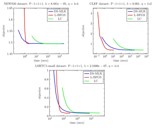
3.3 Data and Model both fit in memory. In each plot, P=N_×M_×T denotes that there areN nodes each running M mpi tasks, with T threads each. λ andη refer to regularization and learning-rate. . . 61

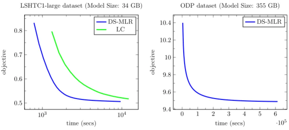
3.4 Data fits and Model does not fit. . . 63

3.5 Data does not fit and Model fits. . . 63

(8)

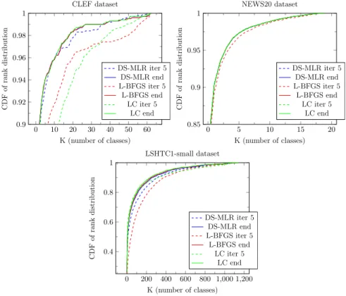
3.7 Cumulative distribution function (CDF) of predictive ranks of the test labels for three sample datasets. DS-MLR performs competitively well within the first 5 iterations. Using roughly 1

4 top-k classes was enough to get a predictive

performance of around 95% in all datasets.. . . 65

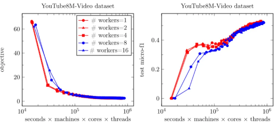
3.8 Scalability analysis of DS-MLR on YouTube8M-Video dataset: Change in objective function and test f1-score vs computation time varying the # of workers (machines).. . . 66

3.9 Scalability analysis of DS-MLR on LSHTC1-large dataset - Change in objective function and test f1-scores vs computation time varying the # of workers (threads). . . 67

4.1 Access pattern of variables during Variational Inference (VI) updates. Green indicates that the variable or data point is being read, while red indicates that the variable is being updated. . . 82

4.2 Access pattern of variables during Stochastic Variational Inference (SVI) updates. Green indicates that the variable or data point is being read, while red indicates that the variable is being updated. . . 83

4.3 Access pattern during ESVI updates. Green indicates the variable or data point being read, while Red indicates it being updated.. . . 84

4.4 Illustration of the communication pattern in ESVI (asynchronous) algorithm. Parameters of same color are in memory of the same worker. Horizontal and Vertical lines indicate the two directions of partitioning data and pa-rameters. Datax is partitioned horizontally alongN and vertically alongD. Local parameterz˜is partitioned horizontally alongN and vertically alongK. Global parameters -π˜ is partitioned vertically along K, and θ˜is partitioned horizontally alongK and vertically alongD. π˜andθ˜are nomadically exchanged. 85 4.5 Comparison of ESVI-GMM, SVI and VI. P = N _×n denotes N machines each with nthreads. . . 89

4.6 Single Machine experiments for ESVI-LDA (Single and Multi core). TOPK refers to our ESVI-TOPK method. P =N_×ndenotesN machines each with nthreads. . . 91

4.7 Multi Machine Multi Core experiments for LDA. TOPK is our ESVI-TOPK method . . . 92

4.8 Predictive Performance of ESVI-LDA. . . 92

4.9 Effect of varying C in ESVI-LDA-TOPK . . . 93

4.10 Effect of varying K by fixing C . . . 94

5.2 Access pattern of parameters while computing G and A. Green indicates the variable or data point being read, while Red indicates it being updated. Observe that computing bothGand A requires accessing all the dimensions j= 1, . . . , D. This is the main synchronization bottleneck. . . 105

5.1 Access pattern of parameters while updating wj and vjk. Green indicates the variable or data point being read, while Red indicates it being updated. Up-datingwj requires computingGi and likewise updatingvjk requires computing aik. . . 105

(9)

5.3 Illustration of the communication pattern in DS-FACTO algorithm. Parame-ters{wj,vj}are exchanged in a de-centralized manner across workers without

the use of any parameter servers [Li et al., 2013]. . . 108

5.4 Convergence behavior of DS-FACTO on diabetes, housing and ijcnn1 datasets. . . 111

5.5 Predictive Performance - Test RMSE (Regression) and Test Accuracy (Classi-fication) of DS-FACTO ondiabetes,housing and ijcnn1 datasets. . . 112 5.6 Scalability of DS-FACTO as # of threads, cores are varied as 1, 2, 4, 8, 16, 32.113

B.1 Comparison of RoBiRank with other baselines (Identity Loss and Robust Loss), see Section B.0.1 . . . 143

B.2 Performance of RoBiRank based on different initialization methods . . . 145

C.1 Comparison of RoBiRank, RankSVM, LSRank [Le and Smola, 2007], Inf-Push and IR-Push . . . 148

C.2 Comparison of RoBiRank, MART, RankNet, RankBoost, AdaRank, CoordAs-cent, LambdaMART, ListNet and RandomForests . . . 149

(10)

List of Tables

1.1 Table to show how popular machine learning tasks - Multinomial Logistic Regression (MLR), Latent Collaborative Retrieval (LCR), and Factorization Machines (FM) fit into the regularized risk minimization framework. For each task, the table shows the corresponding dataX and model θ matrices involved. ColumnsFXemp(θ)andR(θ)show the corresponding data likelihood

and regularizer terms. N andD denote the number of examples and features respectively. K denotes the number of classes in case of MLR and the number

of latent dimensions in case of factorization models such as LCR and FM. . . 4

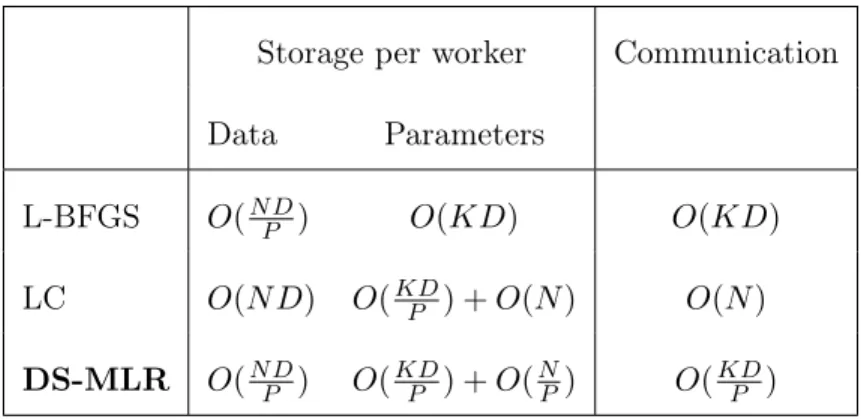
3.1 Memory requirements of various algorithms in MLR (N: number of data points,D: number of features,K: number of classes, P: number of workers). 41 3.2 Notations for Multinomial Logistic Regression . . . 50

3.3 Characteristics of the datasets used . . . 60

4.1 Applicability of the three bayesian inference algorithms - Variational Inference (VI), Stochastic Variational Inference (SVI) and Extreme Stochastic Variational Inference (ESVI) to common scenarios in distributed machine learning. . . 69

4.2 Notations for Mixture of Exponential Family Model. ∼denotes variational parameters. . . 75

4.3 Data Characteristics . . . 88

5.1 Notations for Factorization Machines . . . 102

5.2 Dataset Characteristics. . . 110

B.1 Comparison of RoBiRank against Identity Loss and Robust Loss as described in Section B.0.1. We report overall NDCG for experiments on small-medium datasets, while on the Million Song Dataset (MSD) we report Precision@1.. . 142

C.1 Descriptive Statistics of Datasets and Experimental Results presented in Section 2.2.5. . . 147

(11)

Abstract

Hybrid-Parallel Parameter Estimation for Frequentist and Bayesian Models

by

Parameswaran Raman

Distributed algorithms in machine learning follow two main flavors: horizontal partitioning, where the data is distributed across multiple slaves and vertical partitioning, where the model parameters are partitioned across multiple machines. The main drawback of the former strategy is that the model parameters need to be replicated on every machine. This is problematic when the number of parameters is very large, and hence cannot fit in a single machine. This drawback of the latter strategy is that the data needs to be replicated on each machine, thus failing to scale to massive datasets.

The goal of this thesis is to achieve the best of both worlds by partitioning both -the data as well as -the model parameters, thus enabling -the training of more sophisticated models on massive datasets. In order to do so, we exploit a structure that is observed in

several machine learning models, which we term asDouble-Separability. Double-Separability

basically means that the objective function of the model can be decomposed into independent sub-functions which can be computed independently. For distributed machine learning, this implies that both data and model parameters can partitioned across machines and stochastic updates for parameters can be carried out independently and without any locking. Furthermore, double-separability naturally lends itself to developing efficient asynchronous

(12)

algorithms which enable computation and communication to happen in parallel, offering further speedup.

Some machine learning models such as Matrix Factorization directly exhibit double-separability in their objective function, however the majority of models do not. My work explores techniques to reformulate the objective function of such models to cast them into double-separable form. Often this involves introducing additional auxiliary variables that have nice interpretations. In this direction, I have developed Hybrid Parallel algorithms

for machine learning tasks that includeLatent Collaborative Retrieval,Multinomial Logistic

Regression, Variational Inference for Mixture of Exponential Families and Factorization Machines. The software resulting from this work are available for public use under an open-source license.

(13)

To my parents,

(14)

Acknowledgments

I would first and foremost like to thank my advisor, Professor S.V.N. Vishwanathan (Vishy) who taught me all the theoretical and practical aspects of research over the past years. I could not have asked for a better advisor who could patiently identify my bad habits and push me continuously to fix them. I have admired his tenacity in thinking about problems and perfection in all aspects of research such as implementing a piece of code, systematic debugging, writing and teaching a topic to a new audience. I have picked up numerous valuable nuggets of learnings by working with him that will help me throughout my professional career going forward.

I also would like to thank the readers of my thesis Professor Manfred Warmuth and Professor David Helmbold for giving me useful comments to improve the dissertation. I especially thank Manfred for guiding me during the last segment of my PhD journey and being available whenever I needed help. Manfred’s engaging technical discussions and fun personality attributed in a lot of ways to having an enjoyable and technically enriching experience in the lab.

I would also like to express my utmost gratitude to my collaborators. I especially thank Hyokun Yun for playing the role of a great mentor to me during the first year of my PhD and also being available for discussions in the later stages of the project. I was also fortunate to work with Professor Shin Matsushima from whom I learnt a lot about stochastic optimization and distributed numerical programming. I also would like to thank Xinhua Zhang for his guidance on the experimental setup and convergence analysis. I thank Sriram Srinivasan for his hard work in refactoring the NOMAD code base and helping with running

(15)

the DS-MLR experiments. I was fortunate to work with incredibly smart and industrious collaborators on the ESVI project. I thank Jiong Zhang, Hsiang-Fu Yu, Professor Shihao Ji and Professor Inderjit Dhillon for their valuable contributions and guidance.

No PhD journey can be successful without supportive lab mates. I would like to whole-heartedly thank all my wonderful lab mates at Purdue University and UC Santa Cruz who were not only supportive colleagues but also great friends. I thank Pinar Yanardag, Jiasen Yang and Joon Hee Choi from my Purdue days. I spent the most significant chunk of my PhD life at UC Santa Cruz and my tenure in the ML Lab at UCSC would remain very memorable to me. I would like to thank - Michal Derezinski, Holakou Rahmanian, Ehsan Amid, Andrei Ignat, Kuan-Sung Huang and Bernardo Gonzalez Torres. Not only were they a constant sound-board for brainstorming and providing critical feedback on my work, but also were the most cheerful and fun colleagues I could imagine to work with. I also thank Sabina Tomkins and Dhanya Sridhar from the LINQS lab for helpful comments at various times during my PhD. I also thank Sriram Srinivasan and Varun Embar for being wonderful roommates during my stay in Santa Cruz. Finally, I thank Akash Kumar for all the support and motivation he provided me as a friend during my PhD. We both have had a similar career path and started our PhD journey together at Purdue University. The countless technical discussions and several lighter moments we have had outside the academic life have helped me immensely.

I also thank Shweta Jain, Suman Bora, Caleb Levy, Andrew Stolman and Professor Seshadhri Comandur (Sesh) from the Theory Group at UC Santa Cruz from whom I gained a lot of knowledge on various topics of theory and algorithms. I express my gratitude to Sesh

(16)

for providing me several valuable comments on the draft of the DS-MLR paper which helped me restructure the paper better to suit the audience. I am also grateful to him for giving me feedback on my conference practice talks.

In addition, I feel extremely privileged to have worked with several great researchers during my summer internships. I would like to thank Viet-Ha Thuc and Shakti Sinha for providing me great mentorship during my internship at LinkedIn. I thank Sathiya Keerthi and Dhruv Mahajan for providing me the opportunity to work on a novel exploratory research problem at Microsoft (Cloud Information Services Lab). I would also like to thank Hung Bui and Branislav Kveton who were my mentors at Adobe Research. Hung was a source of immense knowledge on Graphical Models and Variational Inference, and I got diverse perspectives on these topics working with him. Finally, I thank Anima Anandkumar and Alex Smola for providing me the wonderful experience of working in the Amazon AI lab.

My sincere gratitude also goes to my manager at Yahoo!, Santhosh Srinivasan who supported my decision to quit my full-time job at Yahoo! and follow my passion to pursue my PhD. Santhosh has since then been a tremendous mentor to me.

I thank my friends Gayathri and Sanjay for all the fun moments and essential distractions along the way. Thanks to my wife Tejasi for believing in me and motivating me every day during the last, crucial leg of my PhD. She has patiently listened to all my rants and helped me make decisions every time I felt I was directionless. Last but definitely not the least, my deepest gratitude goes to my parents. They have supported all my career decisions wholeheartedly and I dedicate this thesis to them.

(17)

Chapter 1

Introduction

A wide variety of machine learning tasks can be posed as a regularized

risk-minimization problem. That is, one would like to solve,

min

θ L(θ) :=λR(θ) +F

emp

X (θ) (1.1)

where, FXemp(θ) is called the empirical data likelihood and can be often decomposed into a

finite summation over the observed dataX. _R(θ)is a regularizer that controls the complexity

of the model parameters θ. λis a hyper-parameter used to trade-off between the two terms.

For ease of optimization, R(·) is assumed to be a smooth, convex function such as kθk2

2.

The regularized risk-minimization framework described by (1.1) generalizes a wide variety of

popular tasks in large-scale machine learning. With a suitable choice of dataX, modelθand

regularizerR(θ), these tasks can be expressed as a regularized risk minimization problem.

In this work we will concern ourselves with a subset of such tasks where both the data as well as the model are in the form of a matrix. In the literature, these are also referred to as

(18)

• Multinomial Logistic Regression (MLR): We are given N data points (xi, yi)_i₌₁_,...,N,

where each data point xi is a D-dimensional feature vector and yi is the

corre-sponding label which can take values in {1, . . . , K}. K denotes the total number

of classes. For this model, the objective function is equivalent to minimizing the

negative log probability of the target labels yi being assigned class k, and this

decom-poses into FXemp(W) = −N1

PN i=1 PK k=1yikwkTxi + N1 PN i=1log PK k=1exp wTkxi and R(W) = 1₂PK

k=1kwkk22, whereW∈RD×K are the model parameters.

• Latent Collaborative Retrieval (LCR): In this setting, we aim to learn a score function

f(x, y)between a userxand itemywithout an explicit feature vectorφ(x,y), by

embed-ding each userxand itemyinto a low-dimensional euclidean latent space. Observed data

consists of ratingsrxy observed for userxand itemypairs. These ratings could be either

explicit (scale of 1-5) or implicit (clicks, interaction). The score function is then defined

asf(x, y) =hUx,Vyi, whereUxandVy are the latent representations of the userxand

itemyrespectively. A similar pairwise ranking loss can be defined as in the case of

learn-ing to rank. Thus, FXemp(U,V) =

P

x∈X

P

y∈YrxyPy0_∈Y_,y0₆₌_yσ(f(x, y)−f(x, y0))

and the regularizer is given by R(U,V) = 1₂ kUk2

2+kVk22

. The model parameters

to be learnt are U_∈RD×K and V_∈RD×K.

• Factorization Machines (FM): Factorization Machines proposed by [Rendle, 2010]

combine the advantages of SVMs and factorization models. The score function in FM

is parameterized using, both a linear model w ∈ RD as well as a factorized model

V_∈RD×K. The factorized modelVis used to capture all pairwise interactions between

(19)

labels y _∈ RN. D_∗ denotes the total number of features that include the linear

interactions as well as pairwise interactions, i.e. D_∗=_OD+D₂2. The score function

for an observationxis given byf(x) =w0+hw,xi+PDj=1

PD

j0₌₁

Vj,Vj0x_jx_j0. Using

this, the empirical risk term can be expressed as,FXemp(w,V) = 12

PN

i=1l(f(xi), yi)

and regularizerR(w,V) = 1₂ _kw_k2₂+_kV_k2₂

, wherel(_·)is an appropriate loss function

such as cross-entropyfor binary classification orsquared lossfor regression.

We summarize these tasks more concisely in Table 1.1, where for each task, we list

the corresponding data matrixX, model parametersθ, empirical data likelihood term_F(θ)

and the regularizerR(θ).

1.1 Challenges in distributed machine learning

Traditional optimization methods for distributed machine learning broadly fall into

two categories, namely Data paralleland Model parallel.

Data Parallel: The classic paradigm in distributed machine learning is to perform

data partitioning, using, for instance, a map reduce style architecture. In other words, the data is distributed across multiple workers. At the beginning of each iteration, the master distributes a parameter vector to all the workers, who in turn use this to compute the objective function and gradient values on their part of the data and transmit it back to the master. The master aggregates the results from the workers and updates the parameters, and transmits the updates back to the workers, and the iteration proceeds. The L-BFGS optimization algorithm is used in the master to update the parameters after every iteration [Nocedal and Wright,2006]. The main drawback of this strategy is that the model parameters

(20)

T ask Data ( X ) Mo de l ( θ ) Empirical Data Lik eliho od F emp X ( θ ) Regularizer R ( θ ) MLR X ∈ R N × D W ∈ R D × K − 1 N P N i=1 P K k=1 yik w T kx i + 1 N P N i=1 log P K k=1 exp w T kx i 1 2 P K k=1 k wk k 2 2 LCR X ∈ R N × M U ,V ∈ R D × K P x ∈X P y ∈Y rxy P y 0∈Y ,y 06= y σ h Ux , Vy i − Ux , Vy 0 1 2 k U k 2 2+ k V k 2 2 FM X ∈ R N × D ∗ w ∈ R D,V ∈ R D × K 1 2 P N i=1 l ( f ( x ) ,yi ) 1 2 k w k 2 2+ k V k 2 2 T able 1.1: T able to sho w ho w popular mac hine learning tasks -Multinomial Logistic Regression (MLR), Laten t Collab orativ e Retriev al (LCR), and Fact orization Mac hines (FM) fit in to the regularized risk minimization framew ork. For eac h task , the table sho ws the corresp onding data X and mo del θ matrices in volv ed. Colum ns F emp X ( θ ) and R ( θ ) sho w the corres po nding data lik eliho od and regularizer ter ms. N and D denote the nu m ber of examp les and featu res resp ectiv ely . K denotes the num ber of classes in case of MLR and the num be r of laten t dimensions in case of factoriz ation mo dels suc h as LCR and FM.

(21)

need to be replicated on every machine. This is problematic when the number of classes, and consequently the number of parameters is very large, and hence cannot fit in a single machine.

Model Parallel: An orthogonal approach is to usemodel partitioning. Here, again,

we use a master slave architecture but now the data is replicated across each slave. However, the model parameters are now partitioned and distributed to each machine. During each iteration the model parameters on the individual machines are updated, and some auxiliary variables are computed and distributed to the other workers, which use these variables in

their parameter updates. See the Log-Concavity (LC) methodGopal and Yang [2013] for

an example of such a strategy. The main drawback of this approach, however, is that the data needs to be replicated on each machine, and consequently it does not scale to massive datasets.

X

Data

θ

Model

(a)Data Parallelism(partition dataX, duplicate

parametersθ).

X

Data

θ

Model

(b) Model Parallelism(partition parametersθ,

duplicate dataX).

Figure 1.1: Two orthogonal approaches to distributing computation in machine learning.

Figure 1.1illustrates these two approaches. In the context of Multinomial Logistic

(22)

where N, D and K denote the number of examples, features and classes respectively.

Interpretation of data X and model parametersθ for the other tasks can be found in Table

1.1.

Fundamental Bottleneck in Data-only or Model-onlyparallelism: Machine

learning tasks of today run onhumongous amounts of datainvolving sophisticated models

[Weston et al.,2011], [Cheng et al.,2016], [Prabhu et al.,2018]. The memory requirements for data and model parameters can easily exceed the capacity of a single machine in a commodity

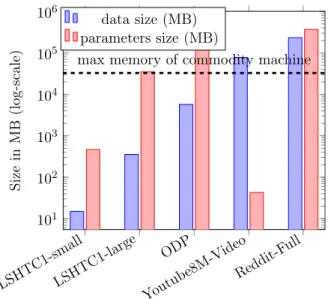
cluster. Figure 1.2 illustrates this fundamental challenge in the context of Multinomial

Logistic Regression (MLR). LSHTC1-smallLSHTC1-large ODP Youtub e8M-Vi deo Reddit-F ull 101 102 103 104 105 106

max memory of commodity machine

Size in MB (log-scale) data size (MB) parameters size (MB)

Figure 1.2: Data and Model requirements (MB) of real-world datasets for Multinomial Logistic Regression (MLR).

As depicted in the figure, real-world datasets exhibit varying storage requirements for the data and model. While the smaller datasets can be easily run on a single machine, larger datasets such as ODP and Reddit-Full are impossible to run on a commodity cluster

(23)

with just traditional data or model parallel approaches. This is because ODP has a massive requirement of 355 GB for the model itself, while Reddit-Full dataset is even bigger, requiring 228 GB for the data and 358 GB for its model. For instance, if we were to run the MLR task on ODP dataset using data parallelism with a modest 4 units of parallelism (cores or threads)

on a single machine, this would require a total memory footprint of4_×355GB _≈1.38 TB

on a single machine. Using a similar configuration to run MLR on the Reddit-Full dataset,

the per-machine memory footprint for data parallel methods is≈1.39TB and model parallel

methods is ≈912 GB. Thus, the number of parallel units we can use on a single machine is

heavily limited if we choose to replicate onlyone of the data or model. Inspired by these

challenges, in this thesis we explore the following broad question,

How can we achieve the best of both worlds?

i.e. Can we achieve both data as well as modelparallelism simultaneously?

X

Data

θ

Model

Figure 1.3: Hybrid Parallelismpartitions bothdataandmodel parameterssimultaneously

without needing to duplicate either of them.

As an answer to this, we proposeHybrid Parallelism, which is the idea of partitioning

(24)

such that there is no overlap is computation among the workers. This enables us to scale to workloads with arbitrary data and model sizes.

1.2 Hybrid Parallelism

A natural question that arises is - Can all machine learning models be made Hybrid

Parallel? To answer this question, we first introduce the notion ofDouble Separability. Double Separability is an attractive property in the objective functions of machine learning models which makes them naturally amenable to Hybrid Parallelism.

1.2.1 Double Separability

The concept of Separability [Zhong et al.,2004] of functions is well-known in the

optimization community [Tseng and Mangasarian, 2001]. Given a family of sets {Si}Ni=1,

a function f : QN

i=1Si → R is separable if there exist functions fi : Si → R for each

i= 1,2, . . . , Nsuch thatf(θ) =PN

i=1fi(θi)whereθi∈Si. Extending the idea of separability

[Zhong et al.,2004] of functions which is well-known in the optimization community [Tseng and Mangasarian,2001], Double-Separabilityis formally defined as follows,

Definition 1. Double Separability Let _{Si}m_i₌₁ and {S0_j}m

0

j=1 be two families of sets of param-eters. A function f :Qm

i=1Si×Qm

0

j=1S0j →R is doubly separable if ∃ fij :Si×S0j →R for

eachi= 1,2, . . . , m andj = 1,2, . . . , m0 such that:

f(θ1, θ2, . . . , θm,θ01, θ02, . . . , θ0m0) = m X i=1 m0 X j=1 fij(θi,θj0) (1.2)

In simple words, if a functionf in two set of parametersθandθ0 can be decomposed

(25)

x x x x x _x x x x x x _x x m m0 fij(θi,θj0)

Figure 1.4: Diagram to illustrate the decomposability of doubly-separable functionf. The

highlighted diagonal blocks can be computed be computed independently and in parallel

since they do not involve overlapping parametersθ andθ0.

a pair of parameters (θi,θ0j), one from each set, then the function f is said to be

doubly-separable. One can think of these sub-functions fij as cells in a matrix of computations

as illustrated in Figure 1.4. For each (i, j) in the diagonal blocks, fij can be computed

independentlyand inparallelas it has no overlap in terms of access-patterns of parameters θ

andθ0. One can think of the dimensions mand m0 as the dimensions for data and model

parallelism respectively. The values of mand m0 differ depending on the machine learning

task at hand.

Frequentist Models: In multinomial logistic regression (MLR) for instance, the

data partitioning occurs across the examples N while the model partitioning occurs across

the classes K. Thus, m =N andm0 =K. On the other hand, in factorization machines

(26)

m0 =D.

Bayesian Models: Bayesian Models can also benefit from Hybrid Parallelism.

Mixture of exponential families model the observations as arising from a generative process as follows:

• Draw mixing proportions Zi∼∆K, where∆K is a K-dimensional simplex.

• Draw observationsX1, . . . , XN based on the mixing proportions,

Xi|Zi = k ∼ ExpFamily (θk), where ExpFamily(·) refers to an exponential family

distribution such as Gaussian or Multinomial distribution with parameterθk.

Examples of popular models that fall in this category include Latent Dirichlet Allocation

(LDA) andGaussian Mixture Models(GMM). While the data in these mixture models can

be partitioned across N, the model can be partitioned across theK mixture components.

Thus, m=N andm0=K.

1.2.2 Achieving Double-Separability in objective functions

Objective functions of some machine learning models such as Matrix Factorization aredirectlydoubly-separable [Yun et al.,2013]. Assuming the data matrixX is factorized

into low-rank matrices W _∈ RN×K and H _∈ RM×K, where N and M are the number of

users and items respectively, we can express the objective function of matrix factorization as,

L(w1,w2, . . . ,wN,h1,h2, . . . ,hM) = 1 2 N X i=1 M X j=1 (Xij − hwi,hji)2 (1.3)

which is directly in the doubly-separable form given in eqn (1.2). This make it easy to make

(27)

are much more complicated and do not exhibit direct double-separability. They require

reformulatingthe original objective function in order to be converted into a desirable form

such as given in eqn (1.2).

The goal of this thesis is to study such reformulations for frequentist and bayesian models to make them hybrid parallel.

1.3 Overview of the chapters

We now sketch the contents of the main chapters of this dissertation (each chapter

will have a separate more detailed introduction). The main results of Chapter 2, Chapter3

and Chapter 4 have been published at NIPS 2014 [Yun et al.,2014a], KDD 2019 [Raman

et al.,2019b] and AISTATS 2019 [Zhang et al.,2019] conferences respectively. Chapter 5

will be published on arXiV as a pre-print. Chapters 2,3 and 5 will appear together as a

journal submission.

1.3.1 Chapter 2: Latent Collaborative Retrieval

We propose RoBiRank - a Learning to Rank algorithm inspired by Robust Binary Classification and show that it scales well on large-data. The main idea behind Robust Binary Classification is to use transformation on convex losses to help give up performance on

hard to classify data points (outliers). Firstly, we observe that this is related to learning to

rank, where we would not mind sacrificing accuracy at the bottom of the ranking list in order to gain performance at top of the list. We thus show that our ranking objective function can

(28)

is equivalent to directly maximizing DCG (a popular evaluation metric for listwise learning

to rank). As a result, RoBiRank performs really well at the top of the list. Thirdly, using a

linearization trick on our loss allows us to obtain an unbiased stochastic gradient estimator so that our SGD optimizer becomes independent of the size of the dataset. In addition, our algorithm is parallelizable and can also be used to solve large-scale problems without any explicit features. Experimental results are shown on both medium and very large datasets.

1.3.2 Chapter 3: Multinomial Logistic Regression

We study the problem of scaling Multinomial Logistic Regression (MLR) to datasets with very large number of data points in the presence of large number of classes. At a scale where neither data nor the parameters are able to fit on a single machine, we argue that

simultaneous data and model parallelism (Hybrid Parallelism)is inevitable. The key challenge in achieving such a form of parallelism in MLR is the log-partition function which needs to

be computedacross all K classes per data point, thus making model parallelism non-trivial.

To overcome this problem, we propose a reformulation of the original objective

that exploits double-separability, an attractive property that naturally leads to hybrid

parallelism. Our algorithm (DS-MLR) isasynchronous and completely de-centralized, requiring

minimal communication across workers while keeping both data and parameter workloads

partitioned. Unlike standard data parallel approaches, DS-MLRavoids bulk-synchronization

by maintaining local normalization terms on each worker and accumulating them incrementally using a token-ring topology.

We demonstrate the versatility of DS-MLR under various scenarios in data and model parallelism, through an empirical study consisting of real-world datasets. In particular,

(29)

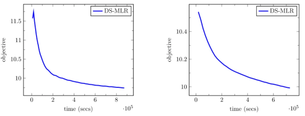
to demonstrate scaling via hybrid parallelism, we created a new benchmark dataset (Reddit-Full) by pre-processing 1.7 billion reddit user comments spanning the period 2007-2015.

We used DS-MLR to solve an extreme multi-class classification1 _{problem of classifying 211}

million data points into their corresponding subreddits. Reddit-Full is a massive data set with data occupying 228 GB and 44 billion parameters occupying 358 GB. To the best of our knowledge, no other existing methods can handle MLR in this setting.

1.3.3 Chapter 4: Mixture of Exponential Families

Mixture of exponential family models are among the most fundamental and widely used statistical models. Stochastic variational inference (SVI), the state-of-the-art algorithm for parameter estimation in such models is inherently serial. Moreover, it requires the parameters to fit in the memory of a single processor; this poses serious limitations on scalability when the number of parameters is in billions. In this work, we present extreme stochastic variational inference (ESVI), a distributed, asynchronous and lock-free algorithm to perform variational inference for mixture models on massive real world datasets. ESVI overcomes the limitations of SVI by requiring that each processor only access a subset of the data and a subset of the parameters, thus providing data and model parallelism simultaneously. Our empirical study demonstrates that ESVI not only outperforms VI and SVI in wallclock-time, but also achieves a better quality solution. To further speed up computation and save memory when fitting large number of topics, we propose a variant

ESVI-TOPK which maintains only the topk_∈K important topics. Empirically, we found

1

Extreme classification is defined as multi-class / multi-label classification in the presence of very large number of examples and classes / labels.

(30)

that using top 25% topics suffices to achieve the same accuracy as storing all the topics.

1.3.4 Chapter 5: Factorization Machines

Factorization Machines (FM) are powerful class of models that incorporate higher-order interaction among features to add more expressive power to linear models. They have been used successfully in several real-world tasks such as click-prediction, ranking and recommender systems. Despite using a low-rank representation for the pairwise features, the memory overheads of using factorization machines on large-scale real-world datasets

can be prohibitively high. For instance on the criteo tera dataset, assuming a modest128

dimensional latent representation and109 _{features, the memory requirement for the model is}

in the order of 1 TB. In addition, the data itself occupies 2.1 TB. Traditional algorithms

for FM which work on a single-machine are not equipped to handle this scale and therefore, using a distributed algorithm to parallelize the computation across a cluster is inevitable. In this work, we propose a hybrid-parallel stochastic optimization algorithm DS-FACTO, which partitions both the data as well as parameters of the factorization machine simultaneously. Our solution is fully de-centralized and does not require the use of any parameter servers. We present empirical results to analyze the convergence behavior, predictive power and scalability of DS-FACTO.

(31)

Chapter 2

Latent Collaborative Retrieval

2.1 Introduction

Learning to rank (LTR) is a problem of ordering a set of items according to their

relevances to a given context [Chapelle and Chang,2011]. While a number of approaches

have been proposed in the literature, in this chapter we provide a new perspective by showing a close connection between ranking and a seemingly unrelated topic in machine learning, namely, robust binary classification.

In robust classification [Huber, 1981], we are asked to learn a classifier in the

presence of outliers. Standard models for classification such as Support Vector Machines (SVMs) and logistic regression do not perform well in this setting, since the convexity of their

loss functions does not let them give up their performance on any of the data points [Long

and Servedio, 2010]; for a classification model to be robust to outliers, it has to be capable of sacrificing its performance on some of the data points. We observe that this requirement is very similar to what standard metrics for ranking try to evaluate. Discounted Cumulative

(32)

Gain (DCG) [Manning et al.,2008] and its normalized version NDCG, popular metrics for learning to rank, strongly emphasize the performance of a ranking algorithm at the top of the list; therefore, a good ranking algorithm in terms of these metrics has to be able to give up its performance at the bottom of the list if that can improve its performance at the top.

In fact, we will show that DCG and NDCG can indeed be written as a natural generalization of robust loss functions for binary classification. Based on this observation we formulate RoBiRank, a novel model for ranking, which maximizes the lower bound of

(N)DCG. Although the non-convexity seems unavoidable for the bound to be tight [Chapelle

et al., 2008], our bound is based on the class of robust loss functions that are found to

be empirically easier to optimize [Ding, 2013]. Indeed, our experimental results suggest

that RoBiRank reliably converges to a solution that is competitive as compared to other representative algorithms even though its objective function is non-convex.

While standard deterministic optimization algorithms such as L-BFGS [Nocedal

and Wright,2006] can be used to estimate parameters of RoBiRank, to apply the model to large-scale datasets a more efficient parameter estimation algorithm is necessary. This is of

particular interest in the context of latent collaborative retrieval [Weston et al.,2012]; unlike

standard ranking task, here the number of items to rank is very large and explicit feature vectors and scores are not given.

Therefore, we develop an efficient parallel stochastic optimization algorithm for this problem. It has two very attractive characteristics: First, the time complexity of each stochastic update is independent of the size of the dataset. Also, when the algorithm is distributed across multiple number of machines, no interaction between machines is required

(33)

during most part of the execution; therefore, the algorithm enjoys near linear scaling. This is a significant advantage over serial algorithms, since it is very easy to deploy a large number of machines nowadays thanks to the popularity of cloud computing services, e.g. Amazon Web Services.

We apply our algorithm to latent collaborative retrieval task on Million Song Dataset [Bertin-Mahieux et al., 2011] which consists of 1,129,318 users, 386,133 songs, and 49,824,519 records; for this task, a ranking algorithm has to optimize an objective function that consists

of386,133_×49,824,519number of pairwise interactions. With the same amount of wall-clock

time given to each algorithm, RoBiRank leverages parallel computing to outperform the state-of-the-art with a 100% lift on the evaluation metric.

2.2 Robust Binary Classification

Suppose we are given training data which consists ofndata points(x1, y1),(x2, y2), . . . ,(xn, yn),

where each xi ∈Rdis a d-dimensional feature vector andyi∈ {−1,+1} is a label associated

with it. A linear model attempts to learn a d-dimensional parameter ω, and for a given

feature vectorx it predicts label+1 ifhx, ωi ≥0 and −1 otherwise. Hereh·,·i denotes the

Euclidean dot product between two vectors. The quality ofω can be measured by the number

of mistakes it makes: L(ω) :=Pn

i=1I(yi· hxi, ωi <0). The indicator functionI(·<0) is called the 0-1 loss function, because it has a value of 1 if the decision rule makes a mistake, and 0 otherwise. Unfortunately, since the 0-1 loss is a discrete function its minimization

is difficult [Feldman et al., 2012]. The most popular solution to this problem in machine

(34)

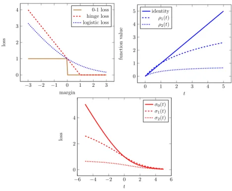
−3 −2 −1 0 1 2 3 0 1 2 3 4 margin loss 0-1 loss hinge loss logistic loss 0 1 2 3 4 5 0 1 2 3 4 5 t function value identity ρ1(t) ρ2(t) −6 −4 −2 0 2 4 6 0 2 4 t loss σ0(t) σ1(t) σ2(t)

Figure 2.1: Left: Convex Upper Bounds for 0-1 Loss. Middle: Transformation functions for constructing robust losses. Right: Logistic loss and its transformed robust variants.

For example, logistic regression uses the logistic loss functionσ0(t) := log2(1 + 2−t), to come

up with a continuous and convex objective function

L(ω) :=

n

X

i=1

σ0(yi· hxi, ωi), (2.1)

which upper bounds L(ω). It is clear that for eachi,σ0(yi· hxi, ωi) is a convex function in

ω; therefore, L(ω), a sum of convex functions, is also a convex function which is relatively

easier to optimize [Boyd and Vandenberghe, 2004]. Support Vector Machines (SVMs) on the

other hand can be recovered by using the hinge loss to upper bound the 0-1 loss. Figure2.1

(left) graphically illustrates three loss functions discussed here.

(35)

[Long and Servedio,2010]. The basic intuition here is that whenyi· hxi, ωi is a very large

negative number for some data point i,σ(yi· hxi, ωi) is also very large, and therefore the

optimal solution of (2.1) will try to decrease the loss on such outliers at the expense of its

performance on “normal” data points.

In order to construct robust loss functions, consider the following two transformation functions:

ρ1(t) := log2(t+ 1), ρ2(t) := 1− 1

log₂(t+ 2), (2.2)

which, in turn, can be used to define the following loss functions:

σ1(t) :=ρ1(σ0(t)), σ2(t) :=ρ2(σ0(t)). (2.3)

One can see that σ1(t) → ∞ as t → −∞, but at a much slower rate than σ0(t) does; its

derivative σ₁0(t) → 0 as t → −∞. Therefore, σ1(·) does not grow as rapidly as σ0(t) on

hard-to-classify data points. Such loss functions are called Type-I robust loss functions by

Ding [2013], who also showed that they enjoy statistical robustness properties. σ2(t) behaves

even better: σ2(t) converges to a constant ast→ −∞, and therefore “gives up” on hard to

classify data points. Such loss functions are called Type-II loss functions, and they also enjoy

statistical robustness properties [Ding,2013].

In terms of computation, of course, σ1(·) andσ2(·)are not convex, and therefore

the objective function based on such loss functions is more difficult to optimize. However,

it has been observed inDing [2013] that models based on optimization of Type-I functions

are often empirically much more successful than those which optimize Type-II functions. Furthermore, the solutions of Type-I optimization are more stable to the choice of parameter

(36)

initialization. Intuitively, this is because Type-II functions asymptote to a constant, reducing the gradient to almost zero in a large fraction of the parameter space; therefore, it is difficult

for a gradient-based algorithm to determine which direction to pursue. See Ding [2013] for

more details.

2.2.1 Ranking Model via Robust Binary Classification (RoBiRank)

In this section, we will extend robust binary classification to formulate RoBiRank, a novel model for ranking.

Let X ={x1, x2, . . . , xn}be a set of contexts, and Y ={y1, y2, . . . , ym}be a set of

items to be ranked. For example, in movie recommender systemsX is the set of users and

Y is the set of movies. In some problem settings, only a subset of Y is relevant to a given

contextx∈ X; e.g. in document retrieval systems, only a subset of documents is relevant to

a query. Therefore, we define Yx⊂ Y to be a set of items relevant to context x. Observed

data can be described by a setW :={Wxy}_x_∈X_,y_∈Y_x whereWxy is a real-valued score given

to itemy in context x.

We adopt a standard problem setting used in the literature of learning to rank. For

each context xand an item y∈ Yx, we aim to learn a scoring functionf(x, y) :X × Yx →R

that induces a ranking on the item set Yx; the higher the score, the more important the

associated item is in the given context. To learn such a function, we first extract joint

features ofx and y, which will be denoted byφ(x, y). Then, we parametrizef(·,·) using a

parameterω, which yields the linear modelfω(x, y) :=hφ(x, y), ωi, where, as before, h·,·i

denotes the Euclidean dot product between two vectors. ω induces a ranking on the set of

(37)

Observe that rankω(x, y) can also be written as a sum of 0-1 loss functions (see e.g.Usunier et al. [2009]): rankω(x, y) = X y0_∈Y_x,y0₆₌_y I fω(x, y)−fω(x, y0)<0. (2.4) 2.2.2 Basic LTR Model

If an item y is very relevant in contextx, a good parameter ω should positiony at

the top of the list; in other words, rankω(x, y) has to be small, which motivates the following

objective function [Buffoni et al.,2011]:

L(ω) := X x∈X cx X y∈Yx v(Wxy)·rankω(x, y), (2.5)

where cx is an weighting factor for each context x, and v(·) : R+ → R+ quantifies the

relevance level ofy onx. Note that _{cx} and v(Wxy) can be chosen to reflect the metric

the model is going to be evaluated on (this will be discussed in Section2.2.3). Note that

(2.5) can be rewritten using (2.4) as a sum of indicator functions. Following the strategy in

Section2.2, one can form an upper bound of (2.5) by bounding each 0-1 loss function by a

logistic loss function:

L(ω) := X x∈X cx X y∈Yx v(Wxy)· X y0_∈Y_x,y0₆₌_y σ0 fω(x, y)−fω(x, y0) . (2.6)

Just like (2.1), (2.6) is convex in ω and hence easy to minimize.

2.2.3 DCG

Although (2.6) enjoys convexity, it may not be a good objective function for ranking.

(38)

at the top of the list than at the bottom, as users typically pay attention only to the top

few items. Therefore, it is desirable to give up performance on the lower part of the list in

order to gain quality at the top. This intuition is similar to that of robust classification in

Section??; a stronger connection will be shown below.

Discounted Cumulative Gain (DCG) [Manning et al., 2008] is one of the most

popular metrics for ranking. For each contextx∈ X, it is defined as:

DCG(ω) :=cx X y∈Yx v(Wxy) log₂(rankω(x, y) + 2) , (2.7)

wherev(t) = 2t−1 andcx= 1. Since1/log(t+ 2)decreases quickly and then asymptotes to

a constant astincreases, this metric emphasizes the quality of the ranking at the top of the

list. Normalized DCG (NDCG) simply normalizes the metric to bound it between 0 and 1

by calculating the maximum achievable DCG valuemx and dividing by it [Manning et al.,

2008].

2.2.4 RoBiRank formulation

Now we formulate RoBiRank, which optimizes the lower bound of metrics for

ranking in form (2.7). Observe that maxωDCG(ω) can be rewritten as

min ω X x∈X cx X y∈Yx v(Wxy)· 1₋ 1 log₂(rankω(x, y) + 2) . (2.8)

Using (2.4) and the definition of the transformation functionρ2(·) in (2.2), we can rewrite

the objective function in (2.8) as:

L2(ω) := X x∈X cx X y∈Yx v(Wxy)·ρ2   X y0_∈Y_x,y0₆₌_y I fω(x, y)−fω(x, y0)<0  . (2.9)

(39)

Since ρ2(·) is a monotonically increasing function, we can bound (2.9) with a

continuous function by bounding each indicator function using the logistic loss:

L2(ω) := X x∈X cx X y∈Yx v(Wxy)·ρ2   X y0_∈Y_x,y0₆₌_y σ0 fω(x, y)−fω(x, y0)  . (2.10)

This is reminiscent of the basic model in (2.6); as we applied the transformation ρ2(·) on

the logistic lossσ0(·) to construct the robust lossσ2(·) in (2.3), we are again applying the

same transformation on (2.6) to construct a loss function that respects the DCG metric used

in ranking. In fact, (2.10) can be seen as a generalization of robust binary classification by

applying the transformation on a group of logistic losses instead of a single loss. In both

robust classification and ranking, the transformationρ2(·)enables models to give up on part

of the problem to achieve better overall performance.

As we discussed in Section ??, however, transformation of logistic loss using ρ2(·)

results in Type-II loss function, which is very difficult to optimize. Hence, instead of ρ2(·)

we use an alternative transformation ρ1(·), which generates Type-I loss function, to define

the objective function of RoBiRank:

L1(ω) := X x∈X cx X y∈Yx v(Wxy)·ρ1   X y0_∈Y_x,y0₆₌_y σ0 fω(x, y)−fω(x, y0)  . (2.11)

Since ρ1(t)≥ρ2(t)for everyt >0, we have L1(ω)≥L2(ω)≥L2(ω)for everyω. Note that

L1(ω)is continuous and twice differentiable. Therefore, standard gradient-based optimization

techniques can be applied to minimize it. As is standard, a regularizer on ω can be added to

(40)

2.2.5 Standard Learning to Rank Experiments

We conducted experiments to check the performance of RoBiRank (2.11) in a

standard learning to rank setting, with a small number of labels to rank. We pitch RoBiRank

against the following algorithms: RankSVM [Lee and Lin,2013], the ranking algorithm of

Le and Smola [2007] (called LSRank in the sequel), InfNormPush [Rudin,2009], IRPush [Agarwal,2011], and 8 standard ranking algorithms implemented in RankLib1 _{namely MART,}

RankNet, RankBoost, AdaRank, CoordAscent, LambdaMART, ListNet and RandomForests.

We use three sources of datasets: LETOR 3.0 [Chapelle and Chang,2011] , LETOR

4.02 _{and YAHOO LTRC [}_{Qin et al.}_,₂₀₁₀_{], which are standard benchmarks for ranking (see}

Table C.1for summary statistics). Each dataset consists of five folds; we consider the first

fold, and use the training, validation, and test splits provided. We train with different values of regularization parameter, and select one with the best NDCG on the validation dataset. The performance of the model with this parameter on the test dataset is reported. For a fair comparison, every algorithm follows exactly the same protocol and uses the same split of data. All experiments in this section are conducted on a computing cluster where each node has two 2.1 GHz 12-core AMD 6172 processors with 48 GB physical memory per node. We used implementation of the L-BFGS algorithm provided by the Toolkit for Advanced

Optimization (TAO)3 _{for estimating the parameter of RoBiRank. For the other algorithms,}

we either implemented them using our framework or used the implementations provided by the authors.

We use values of NDCG at different levels of truncation as our evaluation metric

1_{http://sourceforge.net/p/lemur/wiki/RankLib} 2

http://research.microsoft.com/en-us/um/beijing/projects/letor/letor4dataset.aspx

(41)

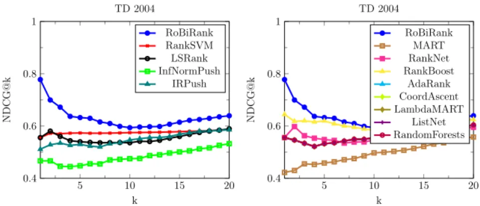
5 10 15 20 0.4 0.6 0.8 1 k NDCG@k TD 2004 RoBiRank RankSVM LSRank InfNormPush IRPush 5 10 15 20 0.4 0.6 0.8 1 k NDCG@k TD 2004 RoBiRank MART RankNet RankBoost AdaRank CoordAscent LambdaMART ListNet RandomForests

Figure 2.2: Comparison of RoBiRank with a number of competing algorithms. [Manning et al.,2008]; see Figure2.2. RoBiRank outperforms its competitors on most of the datasets; due to space constraints, we only present plots for the TD 2004 dataset here and

other plots can be found in AppendixC. The performance of RankSVM seems insensitive to

the level of truncation for NDCG. On the other hand, RoBiRank, which uses non-convex loss function to concentrate its performance at the top of the ranked list, performs much better especially at low truncation levels. It is also interesting to note that the NDCG@k curve of LSRank is similar to that of RoBiRank, but RoBiRank consistently outperforms at each level. RoBiRank dominates Inf-Push and IR-Push at all levels. When compared to standard

algorithms, Figure2.2(right), again RoBiRank outperforms especially at the top of the list.

Overall, RoBiRank outperforms IRPush and InfNormPush on all datasets except TD 2003 and OHSUMED where IRPush seems to fare better at the top of the list. Compared to the 8 standard algorithms, again RobiRank either outperforms or performs comparably to the best algorithm except on two datasets (TD 2003 and HP 2003), where MART and Random Forests overtake RobiRank at few values of NDCG. We present a summary of the

(42)

dataset, some of the additional algorithms like InfNormPush and IRPush did not complete within the time period available; indicated by dashes in the table.

In the MSLR dataset (Figure C.1 in Appendix C), despite the large number of

queries and instances, RoBiRank still manages to outperform its competitors and it follows a trend as expected; having a higher NDCG@1 score, which provides an evidence that it focusses on the most important documents.

2.3 Latent Collaborative Retrieval (LCR)

2.3.1 Basic LCR model

For each context xand an item y_{∈ Y}, the standard problem setting of learning to

rank requires training data to contain feature vector φ(x, y) and scoreWxy assigned on the

x, y pair. When the number of contexts|X |or the number of items |Y| is large, it might be

difficult to defineφ(x, y) and measureWxy for allx, y pairs. Therefore, in most learning to

rank problems we define the set of relevant items Yx ⊂ Y to be much smaller thanY for

each context x, and then collect data only forYx. Nonetheless, this may not be realistic in

all situations; in a movie recommender system, for example, for each userevery movie is

somewhat relevant.

On the other hand, implicit user feedback data is much more abundant. For example, a lot of users on Netflix would simply watch movie streams on the system but do not leave an explicit rating. By the action of watching a movie, however, they implicitly express their preference. Such data consist only of positive feedback, unlike traditional learning to rank

(43)

able to extract feature vectors for eachx, y pair.

In such a situation, we can attempt to learn the score function f(x, y) without a

feature vector φ(x, y) by embedding each context and item in an Euclidean latent space;

specifically, we redefine the score function to be: f(x, y) :=_hUx, Vyi, where Ux ∈Rdis the

embedding of the context x and Vy ∈Rd is that of the item y. Then, we can learn these

embeddings by a ranking model. This approach was introduced in Weston et al.[2012], and

was called latent collaborative retrieval.

Adapting RoBiRank for Latent Collaborative Retrieval

In this section, we show how RoBiRank can be specialized for Latent Collaborative

Retrieval. Let us defineΩto be the set of context-item pairs(x, y)which was observed in the

dataset. Letv(Wxy) = 1if(x, y)∈Ω, and0otherwise; this is a natural choice since the score

information is not available. For simplicity, we setcx = 1for every x. Now RoBiRank (2.11)

specializes to: L1(U, V) = X (x,y)∈Ω ρ1   X y0₆₌_y σ0(f(Ux, Vy)−f(Ux, Vy0))  . (2.12)

Note that now the summation inside the parenthesis of (2.12) is over all items Y instead

of a smaller set Yx, therefore we omit specifying the range of y0 from now on. To avoid

overfitting, a regularizer is added to (2.12); for simplicity we use the Frobenius norm ofU

(44)

2.3.2 Stochastic Optimization

When the size of the data|Ω|or the number of items|Y|is large, however, methods

that require exact evaluation of the function value and its gradient will become very slow

since the evaluation takes O(_|Ω_{| · |Y|}) computation. In this case, stochastic optimization

methods are desirable [Bottou and Bousquet, 2011]; in this subsection, we will develop a

stochastic gradient descent algorithm whose complexity is independent of|Ω_|and_|Y|.

For simplicity, letθ be a concatenation of all parameters _{Ux}x∈X,{Vy}_y_∈Y. The

gradient ∇θL1(U, V)of (2.12) is X (x,y)∈Ω ∇θρ1   X y0₆₌_y σ0(f(Ux, Vy)−f(Ux, Vy0))  .

Finding an unbiased estimator of the gradient whose computation is independent of |Ω_|is

not difficult; if we sample a pair (x, y) uniformly from Ω, then it is easy to see that the

following estimator |Ω| · ∇θρ1   X y0₆₌_y σ0(f(Ux, Vy)−f(Ux, Vy0))   (2.13)

is unbiased. This still involves a summation overY, however, so it requiresO(|Y|)calculation.

Since ρ1(·) is a nonlinear function it seems unlikely that an unbiased stochastic gradient

which randomizes over Y can be found; nonetheless, to achieve convergence guarantees of the

stochastic gradient descent algorithm, unbiasedness of the estimator is necessary [Nemirovski

et al.,2009].

We attack this problem bylinearizingthe objective function by parameter expansion.

Note the following property ofρ1(·) [Bouchard,2007]:

ρ1(t) = log2(t+ 1)≤ −log2ξ+

ξ_·(t+ 1)₋1

(45)

This holds for any ξ >0, and the bound is tight when ξ= _t₊₁1 . Now introducing an auxiliary

parameterξxy for each (x, y)∈Ω and applying this bound, we obtain an upper bound of

(2.12) as L(U, V, ξ) := X (x,y)∈Ω −log₂ξxy+ ξxy P y0₆₌_yσ0(f(Ux, Vy)−f(Ux, Vy0)) + 1 −1 log 2 . (2.15)

Now we propose an iterative algorithm in which, each iteration consists of(U, V)-step and

ξ-step; in the (U, V)-step we minimize (2.15) in(U, V) and in theξ-step we minimize in ξ.

Pseudo-code can be found in Algorithm 1.

(U, V)-step The partial derivative of (2.15) in terms of U and V can be calculated as: ∇U,VL(U, V, ξ) := _{log 2}1 P₍_x,y₎_∈_Ωξxy

P

y0₆₌_y∇U,Vσ0(f(Ux, Vy)−f(Ux, Vy0))

. Now it is easy to see that the following stochastic procedure unbiasedly estimates the above gradient:

• Sample(x, y) uniformly from Ω

• Sampley0 uniformly from _{Y \ {}y_}

• Estimate the gradient by

|Ω_{| ·}(_{|Y| −}1)_·ξxy

log 2 · ∇U,Vσ0(f(Ux, Vy)−f(Ux, Vy0)). (2.16)

Therefore a stochastic gradient descent algorithm based on (2.16) will converge to a local

minimum of the objective function (2.15) with probability one [Robbins and Monro,1951].

Note that the time complexity of calculating (2.16) is independent of |Ω|and |Y|. Also, it is

a function of only Ux and Vy; the gradient is zero in terms of other variables.

ξ-step When U andV are fixed, minimization of ξxy variable is independent of each other

and a simple analytic solution exists: ξxy = P 1

(46)

requires O(_|Y|) work. In principle, we can avoid summation over _Y by taking stochastic

gradient in terms ofξxy as we did for U and V. However, since the exact solution is simple

to compute and also because most of the computation time is spent on(U, V)-step, we found

this update rule to be efficient.

Algorithm 1 Serial parameter estimation algorithm for latent collaborative retrieval

1: η: step size

2: repeat

3: // (U, V)-step

4: repeat

5: Sample(x, y) uniformly fromΩ

6: Sampley0 uniformly from Y \ {y}

7: Ux ←Ux−η·ξxy · ∇Uxσ0(f(Ux, Vy)−f(Ux, Vy0)) 8: V_y ←V_y−η·ξ_xy · ∇_Vyσ₀(f(U_x, V_y)−f(U_x, V_y0)) 9: untilconvergence inU, V 10: // ξ-step 11: for(x, y)_∈Ωdo 12: ξ_xy ← P 1 y06=yσ0(f(Ux,Vy)−f(Ux,Vy0))+1 13: end for

14: untilconvergence inU, V and ξ

2.3.3 Parallelization

The linearization trick in (2.15) not only enables us to construct an efficient

(47)

across multiple number of machines.

Suppose there are p number of machines. The set of contexts _X is randomly

partitioned into mutually exclusive and exhaustive subsets X(1)_,_X(2)_{, . . . ,}_X(p) _{which are}

of approximately the same size. This partitioning is fixed and does not change over time.

The partition on X induces partitions on other variables as follows: U(q) := _{Ux}x∈X(q),

Ω(q):=

(x, y)∈Ω :x∈ X(q) _,_ξ(q) _:=_{_ξ

xy}₍_x,y₎_∈_Ω(q), for 1≤q≤p.

Each machine q stores variables U(q)_,_ξ(q) _and _Ω(q)_{. Since the partition on} _X _is

fixed, these variables are local to each machine and are not communicated. Now we describe

how to parallelize each step of the algorithm: the pseudo-code can be found in Algorithm2.

(U, V)-step At the start of each(U, V)-step, a new partition on_Y is sampled to divide _Y

intoY(1)_,_Y(2)_{, . . . ,}_Y(p) _{which are also mutually exclusive, exhaustive and of approximately}

the same size. The difference here is that unlike the partition onX, a new partition on Y

is sampled for every (U, V)-step. Let us define V(q) :=_{Vy}_y_∈Y(q). After the partition on

Y is sampled, each machine q fetches Vy’s inV(q) from where it was previously stored; in

the very first iteration which no previous information exists, each machine generates and initializes these parameters instead. Now let us defineL(q)(U(q), V(q), ξ(q)) :=

X (x,y)∈Ω(q)_,y_∈Y(q) −log₂ξxy+ ξxy P y0_∈Y(q)_,y0₆₌_yσ₀(f(U_x, V_y)−f(U_x, V_y0)) + 1 −1 log 2 .

In parallel setting, each machineq runs stochastic gradient descent onL(q)(U(q), V(q), ξ(q))

instead of the original functionL(U, V, ξ). Since there is no overlap between machines on the

parameters they update and the data they access, every machine can progress independently of each other. Although the algorithm takes only a fraction of data into consideration at

(48)

a time, this procedure is also guaranteed to converge to a local optimum of the original

function L(U, V, ξ) according to Stratified Stochastic Gradient Descent (SSGD) scheme of

Gemulla et al. [2011]. The intuition is as follows: if we take expectation over the random

partition onY, we have∇U,VL(U, V, ξ) =

q2·E   X 1≤q≤p ∇U,VL(q)(U(q), V(q), ξ(q))  , (2.17)

while the expectation is over the selection of the partition

Y(1)_,_Y(2)_{, . . . ,}_Y(p) _{. Therefore,}

although there is some discrepancy between the function we take stochastic gradient on and the function we actually aim to minimize, in the long run the bias will be washed out and the

algorithm will converge to a local optimum of the objective function L(U, V, ξ). Specifically,

(2.17) ensures that Condition 7 of Theorem 1 inGemulla et al. [2011] is satisfied, while the

rest of conditions can be easily met by introducing anL2 regularizer and thus bounding the

parameter space.

The convergence can be formally proved as follows. We introduce a simplifying

assumption that for each innerrepeat loop in Algorithm 2, each machine executes exactly

the same number of updates, which we will denote byT. Let(x(q),t, y(q),t) be the t-th pair

sampled in machine q. Since updates in in each machine are independent of updates made in

other machines, we can regard that every machine is simultaneously executing (reading or

writing) updates. In other words, each machine p samples an unbiased stochastic gradient

for L(q)(U(q), V(q), ξ(q)).

ξ-step In this step, all machines synchronize to retrieve every entry of V. Then, each

(49)

and cannot be fit into the main memory of a single machine, V can be partitioned as in

(U, V)-step and updates can be calculated in a round-robin way.

Note that this parallelization scheme requires each machine to allocate only 1

p -fraction of memory that would be required for a single-machine execution. Therefore, in terms of space complexity the algorithm scales linearly with the number of machines.

2.3.4 Experiments

In this subsection, we ask the following question: Given large amounts of computa-tional resources, what is the best latent collaborative retrieval model (in terms of predictive performance on the test dataset) that one can produce within a given wall-clock time?

Towards this end, we work with the parallel variant of RoBiRank described in Section 2.3.3.

As a representative dataset we use the Million Song Dataset (MSD) Bertin-Mahieux et al.

[2011], which consists of 1,129,318 users (|X |), 386,133 songs (|Y|), and 49,824,519 records

(|Ω|) of a user x playing a song y in the training dataset. The objective is to predict the

songs from the test dataset that a user is going to listen to4_.

Squared frobenius norm of matrices U and V were added to the objective function

(2.11) for regularization, and the entries of U andV were independently sampled uniformly

from 0 to 1/√d. We performed a grid-search to find the best step size parameter. Since

explicit ratings are not given, NDCG is not applicable for this task; we use precision at 1

and 10 [Manning et al.,2008] as our evaluation metric.

4_{the original data also provides the number of times a song was played by a user, but we ignored this in}

Hybrid-Parallel Parameter Estimation for Frequentist and Bayesian Models

UC Santa Cruz

UC Santa Cruz Electronic Theses and Dissertations

Title

Permalink

Author

Publication Date

Table of Contents

List of Figures

List of Tables

Chapter 1

Introduction

1.1

Challenges in distributed machine learning

1.2

Hybrid Parallelism

1.3

Overview of the chapters

Chapter 2

Latent Collaborative Retrieval

2.1

Introduction

2.2

Robust Binary Classification

2.3

Latent Collaborative Retrieval (LCR)