Efficient Probabilistic Classification Vector Machine
with Incremental Basis Function Selection
Huanhuan Chen,
Member, IEEE,
Peter Tiˇno, and Xin Yao,
Fellow, IEEE
Abstract—Probabilistic classification vector machine (PCVM) [4] is a sparse learning approach aiming to address the stability problems of relevance vector machine (RVM) for classification problems. Since PCVM is based on Expectation Maximization (EM) algorithm, it suffers from sensitivity to initialization, con-vergence to local minima, and limit Bayesian estimation making only point estimates. Another disadvantage is that PCVM was not efficient for large data sets. To address these problems, this paper proposes an efficient probabilistic classification vector machine (EPCVM) by sequentially adding or deleting basis functions according to the marginal likelihood maximization for efficient training. Due to the truncated prior used in EPCVM, two approx-imation techniques, i.e. Laplace approxapprox-imation and expectation propagation, have been used to implement EPCVM to obtain full Bayesian solutions. We have verified Laplace approximation and expectation propagation with hybrid Monte Carlo approach. The generalization performance and computational effectiveness of EPCVM are extensively evaluated. The theoretical discussions using Rademacher complexity reveal the relationship between the sparsity and the generalization bound in EPCVM.
I. INTRODUCTION ANDBACKGROUND
Support vector machine (SVM) [30] and kernel methods are among the most popular learning methods in the machine learning community. Although SVM performs well for a broad range of practical applications, and is widely regarded as the state-of-the-art approach, it suffers from several disadvantages [28], including the non-probabilistic, hard binary decisions, and the number of support vectors grows linearly with the size of the training set, which increases the computational complexity when the problem becomes large.
Relevance Vector Machine (RVM) is a probabilistic learning method that tries to tackle these problems of SVM. RVM intro-duces a zero-mean Gaussian prior over every weight wi and
makes use of Bayesian Automatic Relevance Determination (ARD) framework [19] to obtain a sparse solution. In RVM, all basis functions are included in the model and those irrelevant basis functions will be deleted step by step based on evidence maximization. The necessary training and optimization of the marginal likelihood function is typically much slower. Later on, a highly accelerated RVM [29] has been proposed by optimizing the marginal likelihood function to enable an efficient sequential addition and deletion of candidate basis functions.
However, Chen et al. [4] pointed out that RVM is not robust to kernel parameters due to the inappropriate formulation that adopts zero-mean Gaussian prior over weights for both
The authors are with The Centre of Excellence for Research in Computa-tional Intelligence and Applications (CERCIA), School of Computer Science, University of Birmingham, Birmingham B15 2TT, United Kingdom, email:
{H.Chen, P.Tino, X.Yao}@cs.bham.ac.uk.
positive and negative classes in classification problems, hence some training points that belong to positive class (yi = +1)
may have negative weights and vice versa. Chen et al. [4] demonstrated that RVM is unstable with respect to kernel parameters and might lead to sub-optimal solutions evidenced by empirical and theoretical results.
Probabilistic classification vector machine (PCVM) [4] in-troduced the non-negative, left-truncated Gaussian prior for positive training points (yi = +1) and the non-positive,
right-truncated Gaussian prior for negative training points (yi = −1). A closed form Expectation Maximization (EM)
was used to get a maximum a posteriori (MAP) estimation of parameters in PCVM. However, there are several limitations for the EM implementation. First, EM algorithm is sensitive to initializations and may converge to a local minimum, which will degrade the generalization ability, especially when the investigated problems become large where there are more local minima existing. Second, the EM algorithm can only obtain a MAP estimation of parameters. The MAP estimation is a limit of Bayes estimators under the 0-1 loss functions, but generally not a Bayes estimator per se. Third, EM based PCVM begins by including all basis functions and then pruning those irrelevant basis functions iteratively. Therefore, the algorithm is not appropriate for large data sets due to the computational/memory cost.
In order to address these problems, in this paper we improve PCVM in the following two directions:
• We construct an efficient probabilistic classification vec-tor machine (EPCVM) and approximate the posterior by Laplace approximation (EPCVMLap) and expectation
propagation [21] (EPCVMEP). By using the two integral
approximation techniques, the solution is fully Bayesian, which automatically tackles the first two disadvantages of the EM algorithm. The accuracy of EPCVMLap and
EPCVMEP has been verified by Markov Chain Monte
Carlo (MCMC) algorithm.
• We have improved the PCVM algorithm using marginal likelihood maximization. By incrementally maximizing marginal likelihood, EPCVM can sequentially include basis functions into the models iteratively. This makes EPCVMLap computationally more efficient.
The contributions of this paper can be summarized as follows:
• Unlike SVM, the proposed algorithms, are probabilistic models, producing the probabilistic outputs for new test points.
• Compared with the original PCVM, the two proposed methods, EPCVMLap and EPCVMEP, based on the
integral approximation, are not only more stable with re-spect to initialization, but also yield better generalization performance (on the variety of data sets used).
• By incrementally maximizing marginal likelihood, the methods introduced in this paper reduce the computa-tional complexity of PCVM.
• Due to the sparseness-inducing prior, the model sparsity helps to control model complexity and reduce the com-putational complexity in the teststage.
In sparse classification algorithms, the model is typically regularized by some prior belief about the weights that pro-mote their sparsity. Besides Gaussian prior, Laplace prior that leads to an L1-penalty, analogous to the LASSO penalty for regression [27], is another popular choice. Joint classifier and feature optimization (JCFO) [17] was one of these algorithms using Laplace prior. JCFO was able to optimize the clas-sifier and select the proper feature subsets simultaneously. To promote sparseness, sparse probit classification algorithm [11] adopted the hierarchical prior, i.e. the Jeffreys prior, over the Laplace prior, whose main advantage was able to control the degree of sparseness without prior parameters. However, both JCFO and sparse probit classification were based on expectation maximization algorithm, and they might suffer from the disadvantages, i.e., sensitivity to initialization and convergence to local minima. The above two algorithms are based on the specification of sparseness inducing prior to the weight vectors in parametric models. The sparse model has emerged in ensemble approaches as well. For example, Sun and Yao [26] proposed a sparse learning algorithm through gradient boosting for learning large kernel problems. However, this approach does not produce probabilistic outputs as it employed a greedy forward selection criterion by simply choosing the basis vector with the largest absolute value in the current residual.
Besides the parametric Bayesian models using prior to im-pose sparseness, there are a number of sparse non-parametric Bayesian models, e.g. sparse online Gaussian processes (GP) [6] and the accelerated version: informative vector machine (IVM) [18]. Sparse online Gaussian processes combines a Bayesian online algorithm with a sequential construction of a relevant subsample of the data that fully specifies the pre-diction of the GP model. IVM accelerated the spare GP model by approximating a Gaussian process using forward selection with criteria based on information-theoretic principles.
The rest of this paper is organized as follows. Section II proposes the two EPCVM implementations, followed by the comparisons of MCMC, Laplace approximation and expecta-tion propagaexpecta-tion in Secexpecta-tion III. The experimental results and analysis are reported in Section IV. Section V provides the theoretical discussions on sparsity and generalization. Finally, Section VI concludes the paper and presents future work.
II. EFFICIENTPROBABILISTICCLASSIFICATIONVECTOR
MACHINE
In this section, we will present the model specification for EPCVM in Section II-A, then the prior over weight vectors will be discussed in Section II-B. Section II-C presents
Laplace approximation based EPCVMLapalgorithm, and
Sec-tion II-D details the expectaSec-tion propagaSec-tion based EPCVMEP
algorithm.
A. Model Formulation
Consider binary classification and a data set of input-target training pairs D = {xi, yi}iN=1, where yi ∈ {−1,+1}. In
order to transfer linear outputs to probabilistic outputs, a link function should be chosen to allow a smooth transition between two classes. The EM implementation of PCVM [4] used probit link function, i.e.
ψ(a) = ∫ a
−∞
N(t|0,1)dt,
whereψ(a) is the Gaussian cumulative distribution. In order to be consistent, the probit link function is employed in this paper as well.
Derivations of Laplace approximation become easier when sigmoid link function is used. In this paper, we employ a popular approximation [2] by making use of the similarity between the logistic sigmoid function and the probit link function [3] (pages 218-220), i.e.
σ(λa) = 1
1 +e−λa ≈ψ(a),
where λ=√8/π. The scaling factor λ is chosen to ensure that the probit function and the logistic sigmoid function have the same slope at the origin.
After incorporating the link function, the EPCVM model becomes: p(y= 1|x,w) =ψ(x;w) =ψ (N ∑ i=0 yiwiϕi(x,xi) ) . (1)
where yi ∈ {−1,+1} is the label, y0 and ϕ0(x,x0) are set
to1for convenience. We useyi in Equation (1) to make sure
wi is non-negative. In the following, we denote yiϕi(x) by
ϕyi(x), i.e. Equation (1) will be represented as follows:
p(y= 1|x,w) =ψ (N ∑ i=0 wiϕyi(x,xi) ) .
In Equation (1), we useϕ(·)instead ofK(·)to indicate that basis functions in EPCVM do not need to satisfy Mercer’s condition1.
B. Truncated Prior over Weights
Based on the PCVM formulation [4], a truncated Gaussian prior is introduced for each weight wi and a zero-mean
Gaussian prior is adopted for the bias w0. The priors are
assumed to be mutually independent.
p(w|α) = N ∏ i=1 p(wi|αi) = N ∏ i=1 Nt(wi|0, α−i1), p(w0|α0) = N(w0|0, α0−1),
1It must be the continuous symmetric kernel of a positive integral operator, which can be relaxed slightly to include conditionally positive kernels [25].
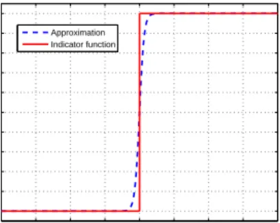
−20 −15 −10 −5 0 5 10 15 20 0 0.1 0.2 0.3 0.4 0.5 0.6 0.7 0.8 0.9 1 Approximation Indicator function
Fig. 1. Comparisons of indicator function and its differentiable approximation
ξβ (β= 3).
where α0 is the inverse variance, Nt(wi|0, α−i1) is a
non-negative, left-truncated Gaussian, and αi is the inverse
vari-ance. This is formalized in Equation (2):
p(wi|αi) =
{
2N(wi|0, αi−1) if wi≥0
0 otherwise
= 2N(wi|0, αi−1)·δ(wi). (2)
whereδ(·)is the indicator function1x≥0(x).
C. Laplace Approximation for EPCVM In EPCVM, the prior is given as
p(w|α) =N(w0|0, α−01)
N
∏
i=1
2N(wi|0, αi−1)·δ(wi)
We follow convention and generalize the model by applying the logistic sigmoid link function, and adopting the Bernoulli distribution for p(t|w), the likelihood is written as follows:
p(t|w) = N ∏ n=1 σtn n [1−σn] 1−tn, where σn =σ ( λ∑Ni=0wiϕyi(xn) ) and we assume y0 = 1
to facilitate the representation, t= [t1,· · · , tN]T is a vector
of targets, tn= yn2+1 ∈ {0,1}is the probabilistic target.
According to Bayes’ theorem, the posterior distribution of weights w can be obtained with the current values of α as follows:
p(w|t) = p(t|w)p(w|α)
p(t|α) .
After incorporating the truncated Gaussian prior, the integral in Bayesian inference is intractable. In order to obtain the posterior, Laplace approximation will be employed to approx-imate the posterior. Laplace approximation is a deterministic approximation algorithm using a Gaussian to represent a given probability.
The most probable weight setting under the posterior, MAP estimate ofw,wM AP can be obtained by maximizing the log
of p(w|t)with respect to the parameters w: Q = log{p(t|w)p(w|α)} −logp(t|α) = N ∑ n=1 [tnlogσn+ (1−tn) log(1−σn)]− 1 2 N ∑ i=0 αiwi2 + N ∑ i=1 logδ(wi)−const.
As the indicator functionδ(·)is not differentiable, a sigmoid link function with β = 3 is employed to replace it, i.e. approximate δ(wi) by ξβ(wi) = σ(βwi) (see Figure 1), the
gradient is ∂Q ∂w =λΦ T(t−σ)−Aw+k, where σ = [σ1,· · ·, σN]T, σn = σ ( λ∑Ni=0wiϕyi(xn) ) ,
A=diag(α0, α1,· · ·, αN)is the(N+ 1)×(N+ 1)diagonal
matrix,k= [0, β(1−σ(βw1)),· · · , β(1−σ(βwN))]T is the
N+ 1 vector.
Setting the gradient to zero and we obtain
wM AP=A−1
(
λΦT(t−σ) +k). (3) The Hessian can be explicitly computed as follows:
∂2Q
∂w2 =−(Φ
TBΦ+A+D),
where B = diag(b1,· · · , bN) and D are diagonal matrices,
where bi =λ2σn(1−σn) and D =diag(0, d1,· · ·, dN) =
diag(0, σ(βw1)(1 − σ(βw1))β2,· · ·, σ(βwN)(1 −
σ(βwN))β2), respectively.
Hence, the posterior covariance is
ΣM AP = (ΦTBΦ+A+D)−1. (4)
The novelty of the derivation in this section is to incorporate the indicator function, i.e.kandDin Equations (3) and (4), to prevent the weight from negative values, i.e. complying with truncated prior.
D. Expectation Propagation for EPCVM
Expectation propagation (EP) [21] is a deterministic frame-workto approximate Bayesian inference. It employs a family of exponential functions to minimize the KL-divergence be-tween the exact term and the approximation term, and then EP combines these approximations analytically to obtain a Gaussian posterior. For a specific problem, such as EPCVM in this paper, plenty of derivations should be performed aiming to minimizing the KL-divergence between the exact term and the approximation term.
In EPCVMEP, the likelihood for the weight vectorw can
be written as p(y|x,w) = N ∏ n=1 p(yn|xn,w) = N ∏ n=1 ψ ( yn N ∑ i=0 wiϕyi(xn) ) .
By incorporating the prior with likelihood, the posterior of weight vectors wis calculated as
p(w|x,y, α) ∝ p(w|α) N ∏ n=1 p(yn|xn,w) = N(w0|0, α−01) N ∏ i=1 2N(wi|0, αi−1)· N ∏ i=1 δ(wi) N ∏ n=1 p(yn|xn,w).
In EP, we need to approximate both the likelihood term p(yn|xn,w) = ψ ( yn ∑N i=0wiϕyi(xn) ) and δ(wi) term. Denote the exact terms gn(w) =
p(yn|xn,w) and ti(w) = δ(wi) = δ(wTei) (where
ei = (0,· · ·,1,0,· · · ,0)T is the standard basis to obtain
the weight wi (wi = wTei)) and the approximate terms
by g˜n(w) = snexp ( − 1 2vn(ynw TΦ(x n)−mn)2 ) = snexp(−2v1 n(w TΦ n − mn)2), where Φ(xn) = [ϕy1(xn),· · ·, ϕyN(xn)]
T and to simplify notation, y
nΦ(xn)
is written as Φn, and ˜ti(w) = siexp(−21v
i(w
Te
i−mi)2).
The EP for PCVM is described in the following.
1) Initialization the prior term: q(w) = p(w|α). Also initialize the approximating terms to 1: g˜n = 1 and
˜
ti= 1:m= 0,v=∞ands= 1.
2) Until both ˜gn and˜ti converge: Loopn= 1, . . . , N, and
i= 1, . . . , N;
a) Remove the approximation term˜gn from the
pos-terior q(w) to obtain the leave-one-out posterior q\n(w): N(m\n w,V\wn). V\wn =Vw+ (VwΦn)(VwΦn)T vn−ΦTnVwΦn , (5) mw\n=mw+ (Vw\nΦn)v−n1(Φ T nmw−mn). (6)
b) Combine q\n(w) and the exact term g
n(w) to
get pˆ(w)∝ q\n(w)g
n(w) and minimize the
KL-divergence betweenpˆ(w)and new posteriorq(w). Zn = ∫ w q\n(w)gn(w)dw=ψ(zn) = ψ (m\wn)TΦn √ ΦT nV\ n wΦn+ 1 . and mw = m\wn+V\ n w ∂logZn ∂m\wn =m\wn+V\wnΦnρn Vw = V\wn+V\ n w ∂∂logm\wZnn ( ∂logZn ∂m\wn )T −2∂logZn ∂V\wn V\wn = V\wn+ (Vw\nΦn) ρn(ΦTnmw+ρn) ΦT nV\ n wΦn+ 1 (V\wnΦn)T, where ρn= 1 √ ΦT nV\ n w Φn+ 1 N(zn; 0,1) ψ(zn) .
c) Update the approximation term g˜n = Zn
q(w)
q\n(w),
vn,mn andsn are obtained as follows:
vn = ΦTnV\ n wΦn ( 1 ρn(ΦTnmw+ρn)− 1 ) + 1 ρn(ΦTnmw+ρn) , mn = (m\wn) TΦ n+ (vn+ ΦTnV\ n wΦn)ρn, sn = ψ(zn) √ ΦT nV\ n wΦnvn−1+ 1· exp ( 1 2 ΦT nV\ n wΦn+ 1 ΦT nmw+ρn ρn ) .
d) Remove the approximation term˜ti from the
pos-terior q(w) to obtain the leave-one-out posterior q\i(w): N(m\i
w,V\
i
w). Refer to the equations (5)
and (6).
e) Combine q\i(w) and the exact term ti(w) to get
ˆ
p(w) = ∫ q\i(w)ti(w)
q\i(w)ti(w)dw and minimize the
KL-divergence KL(ˆp(w)||q(w)) between pˆ(w) and new posterior q(w) subject to the constraint that q(w) is a Gaussian distribution. Zeroing the gra-dient with respect to m\wi and V\wi gives the
conditions [21],
Eq(w)[w] = Epˆ(w)[w],
Eq(w)[wTw] = Epˆ(w)[wTw].
This is the reason why the algorithm is named as expectation propagation. Zi = ∫ w q\i(w)ti(w)dw = ∫ w q\i(w)δ(wTei)dw=ψ(zi) where zi= (m\wi)Tei √ eT iV\ i wei , and ∂logZi ∂m\wi = N(zi) ψ(zi) ei √ eT i V \i wei =gi ∂logZi ∂V\wi = −1 2ρi (m\wi)Tei eT i V\ i wei eieTi =Gi, where ρi= N(zi) ψ(zi) 1 √ eT i V\ i wei .
Based on the theory of expectation propagation [21], mw=m\wi+V\ i w ∂logZi ∂m\wi =m\wi+V\wiρiei, Vw = V\wi+V\ i w(gigTi −2Gi)Vw\i = V\wi+ (V\wiei) ( ρieTimw eT i V \i wei ) (Vw\iei)T,
f) Update the approximation termt˜i=Zi q(w) q\i(w): vi =eTi Viei =eTi V\ i wei ( 1 ρieTimw −1 ) . mi= (m\wi) Te i+ (vi+eTi V\ i wei)ρi, si =ψ(zi) √ eTiVw\ieiv−i 1+ 1 exp ( 1 2 eT i V\ i wei eT imw ρi ) .
Output: The approximated posterior of the weight vector
w
p(w|x,y, α)≈q(w) =N(mw,Vw).
Based on the algorithm, EP approximates each term as a Gaussian distribution, leading to the situation that the likelihood of every training point has similar forms as a regression likelihood term. The likelihood of each data point in EPCVMEP can be obtained as
p(m|w,x) = (2π)−N|Λ|−1/2exp ( −1 2(w TΦ−m t)TΛ−1· (wTΦ−m t) ) , where mt = (m1,· · · , mN) denotes the target point vector,
Λ = diag(v1, . . . , vN), where vn represents the variance
of the noise for the training point n. EP actually maps a classification problem into a regression problem where (mn,vn) defines the virtual observation data point with mean
mnand variancevn. Note that we can compute analytically the
posterior distribution of the weights. The posterior distribution of the weight vector is thus given by:
p(w|x,m, α) = p(m|w,x)p(w|α) p(m|α,x) = exp ( −1 2(w−mw) TV w(w−mw) ) (2π)N|V w|1/2 , where the posterior covariance and mean are:
Vw = (A+ΦΛ−1ΦT)−1, (7)
mw = VwΦΛ−1mt. (8)
whereA=diag(α0,· · · , αN).
1) Leave-one-out Estimation: A nice property of EP is that it can easily obtain an estimate of the leave-one-out error. In each iteration, EP computes the parameters of the approximate leave-one-out posterior q\n(w) (step 2(a)) that
does not depend on the nth data point. So we can use the mean m\wn to approximate a classifier trained on the other
(N −1) data points. Thus an estimate of the leave-one-out error can be obtained as
errloo= 1 N N ∑ n=1 δ(−yn(m\wn) TΦ(x n)). (9)
In practice, the estimation of leave-one-out error will be employed for model selection. The model with the smallest leave-one-out error will be selected instead of the one in the last iteration.
E. Hyperparameters Optimization for EPCVM
Originally, we optimized PCVM by thetop-downapproach [4]. It includes all basis functions in the beginning, and then prunes irrelevant basis functions when the corresponding α′nstending to infinity. However, thetop-down approach will typically consume a lot of computational resources, especially in the beginning of the training. In order to make the algorithm more computationally efficient, we propose to use the con-structiveapproach based on marginal likelihood maximization to include basis functions step by step starting from an empty model. This is different from the greedy forward selection criterion such as MAX-RES [26] that simply chooses the basis vector with the largest absolute value in the current residual.
The previous sections present the training algorithm of EPCVMLap and EPCVMEP with fixed hyperparameterα. In
order to sequentially update α for a practical algorithm, we can maximize the type-II marginal likelihood p(D|α). The fast algorithm to optimize the type-II marginal likelihood is to decompose p(D|α) into two parts, one part denoted by p(D|α\i), that does not depend onαi and another that does,
i.e.,
p(D|α) =p(D|α\i) +l(αi), (10)
wherel(αi)is a function that depends onαi.
The updating rule forαican be obtained with the derivation
of marginal likelihood [9]. The procedure leads to a practical algorithm for optimizing the hyperparameters that has signif-icant speed advantages.
III. LAPLACEAPPROXIMATION, EXPECTATION
PROPAGATION ANDMARKOVCHAINMONTECARLO
Laplace approximation and expectation propagation can be viewed as integral approximation techniques. As the truncated Gaussian prior is used in this paper, the exact posterior distribution is unknown. In this section, we employ Markov Chain Monte Carlo (MCMC) method to sample from the exact posterior distribution for the comparison with Laplace approximation and expectation propagation.
MCMC methods [1] are a class of algorithms for sampling from probability distributions based on constructing a Markov chain that has the desired distribution as its equilibrium distribution. MCMC may be too slow for many practical applications, but has the advantage that it becomes exact in the ‘limit’ of long runs. Thus, MCMC can provide a standard way to measure the accuracy of integral approximation methods, such as Laplace approximation and expectation propagation used in this paper. One popular MCMC algorithm, Metropolis algorithm [1] is sensitive to step size. The sampling result is slow and might exhibit a random-walk behavior with a small step size, whereas the result is inefficient due to a high rejection rate with a large step size.
This paper uses one powerful MCMC algorithms, hybrid Monte Carlo (HMC) algorithm [8] as it incorporates the gra-dient of the log probability with respect to the state variables into sampling process, which is able to make large changes to the system while keeping the rejection probability small.
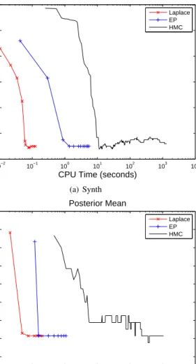
10−2 10−1 100 101 102 103 104 0.08 0.1 0.12 0.14 0.16 0.18 0.2
CPU Time (seconds)
Generalization Error Posterior Mean Laplace EP HMC (a) Synth 10−3 10−2 10−1 100 101 102 103 0.14 0.16 0.18 0.2 0.22 0.24 0.26 0.28
CPU Time (seconds)
Generalization Error Posterior Mean Laplace EP HMC (b) Heart
Fig. 2. The comparisons of Laplace approximation, expectation propagation and hybrid monte carlo (200,0000 sampling points) in terms of generalization error and CPU time.
In our experiments, two data sets, synth2 and heart [22], have been employed in the investigation. In Figure 2, we illustrate the comparisons of the three algorithms, i.e. Laplace, EP and HMC (200,000 sampling points), in terms of the generalization and the computational time. To compare the three algorithms, we do not optimize the hyperparameters in this figure3. The same random initialization is given to the three algorithms. According to Figure 2, Laplace, EP and HMC achieve similar performance. Due to the sampling mechanics, HMC converges slower than Laplace and EP. Laplace uses the least time and HMC has consumed the most time.
In the following experiments, we report the experimental results by incorporating the three algorithms with the hyperpa-rameter optimization by maximizing the marginal likelihood. In HMC, the posterior mean and covariance matrix are
esti-2http://www.stats.ox.ac.uk/pub/PRNN/
3Tthe following experiments will report the three algorithms with the hyperparameter optimization by maximizing the marginal likelihood, see Table I.
TABLE I
COMPARISONS OFMCMC, EPANDLAPLACE APPROXIMATION ON FOUR DATA SETS.
Methods Cancer Diabetics
error AUC #vec CPUTime error AUC #vec CPUTime MCMC 26.61 71.94 12 669.1s 23.17 82.86 23 764.1s
EP 26.65 72.53 9 3.15 23.18 82.89 17 357.16
Laplace 26.71 72.03 16 0.23s 23.11 83.12 22 1.06s
Methods Heart Thyroid
error AUC #vec CPUTime error AUC #vec CPUTime MCMC 16.37 90.67 16 707.4s 4.94 98.71 22 913.1s
EP 16.65 90.91 13 254.65 5.16 98.63 10 61.18 Laplace 16.65 90.83 15 0.28 5.02 98.87 21 0.21s
mated using the sampling points. The same hyperparameter optimization procedures described in Section II-E are em-ployed in HMC. The four data sets, including Cancer, Diabet-ics, Heart and Thyroid, from UCI machine learning repository are employed to show the difference between HMC, Laplace approximation and expectation propagation. The summary of these data sets can be referred in Table II. The resulting model and the classification performance are shown in Table I.
From the table, Laplace approximation, expectation propa-gation and MCMC achieve similar performances in terms of both generalization error and model size. Of course, Laplace approximation is much less time consuming than HMC.
Both figures and table indicate that Laplace approximation and EP approximate the posterior well with truncated Gaussian priors for the two classification problems. It also demonstrates that Laplace approximation is more efficient than EP and HMC in the current experimental settings. In the following section, we will conduct extensive experiments to compare Laplace approximation, EP and other algorithms.
IV. EXPERIMENTALSTUDIES
First, we present experimental results of EPCVM, RVM and SVM on two synthetic data sets in order to understand the behaviors of these algorithms. Second, we carry out extensive experiments on 13 benchmark data sets using the error rate (ERR) and the area under the curve of receiver operating characteristic (AUC). Then, we present detailed statistical tests over multiple data sets for multiple classifiers. Finally, the algorithmic complexity of EPCVM and its application to a relatively large data set have been reported.
A. Synthetic Data Sets
In the first experiment, we compare EPCVMLap, SVM [30]
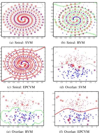
and RVM [28] on two synthetic data sets. In order to facilitate further reference, each data set will be named according to its characteristics. Spiral can only be separated by highly non-linear decision boundaries.Overlapcomes from two Gaussian distributions with equal covariance, and is expected to be sep-arated by a linear plane. This experiment employs a Gaussian RBF kernel as the basis function.
The parameters of SVM including the regularization param-eterC and the kernel parameterθare selected by grid search
−0.8 −0.6 −0.4 −0.2 0 0.2 0.4 0.6 0.8 −1 −0.8 −0.6 −0.4 −0.2 0 0.2 0.4 0.6 0.8 1 (a) Spiral: SVM −0.8 −0.6 −0.4 −0.2 0 0.2 0.4 0.6 0.8 −1 −0.8 −0.6 −0.4 −0.2 0 0.2 0.4 0.6 0.8 1 (b) Spiral: RVM −0.8 −0.6 −0.4 −0.2 0 0.2 0.4 0.6 0.8 −1 −0.8 −0.6 −0.4 −0.2 0 0.2 0.4 0.6 0.8 1 (c) Spiral: EPCVM −2 −1.5 −1 −0.5 0 0.5 1 1.5 2 −1 −0.5 0 0.5 1 1.5 (d) Overlap: SVM −2 −1.5 −1 −0.5 0 0.5 1 1.5 2 −1 −0.5 0 0.5 1 1.5 (e) Overlap: RVM −2 −1.5 −1 −0.5 0 0.5 1 1.5 2 −1 −0.5 0 0.5 1 1.5 (f) Overlap: EPCVM Fig. 3. Comparison of classification of synthetic data sets using a RBF kernel. Two classes are shown as dots and crosses. The separating lines are obtained by projecting test data over a grid. Kernel and regularization parameters for SVM, RVM and EPCVM are obtained by 10-fold cross validation
with 10-fold cross validation4. The kernel parameters θ of EPCVMLapand RVM are selected by 10-fold cross validation.
In Figures 3 we present the decision boundaries of three algorithms. We observe a similar performance of EPCVMLap
and SVM in the case of Spiral. RVM cannot obtain the correct decision boundary due to the highly non-linear data set. The failure indicates that the prior of RVM produces excessive sparseness in the outer part of data, leading the boundary biasing towards outer circle and hence producing errors. EPCVMLap produces “nearly linear” decision
bound-ary in Overlap and RVM gives analogously curving decision boundary, whereas SVM gives a more curved boundary. We also notice that SVM uses the largest number of support vectors and RVM uses the smallest number of support vectors. EPCVMLap seems to have reasonable vectors to achieve the
tradeoff between model size and performance.
The results of EPCVMLap are promising on the two
syn-thetic data sets. EPCVMLap not only handles the data sets
with a predominating linear decision boundary, e.g. Overlap, but also be applied to the highly non-linear data sets, e.g. Spiral.
4The ranges of cross validation search for SVM areC∈ {1,3,· · ·,100} andθ∈ {0.1,0.3,· · ·,10}(The data has been normalized to unit standard deviation.) in both synthetic data sets and benchmark data sets. The same search rangeθ∈ {0.1,0.3,· · ·,10} has been used for EPCVM and RVM in both synthetic data sets and benchmark data sets.
TABLE II
SUMMARY OF13 BENCHMARKDATASETS.
Data No. Train No. Test Positive % Negative % Dim
Abalone 2089 2088 50.18% 49.82% 8 Banana 2650 2650 44.83% 55.17% 2 Cancer 132 131 29.28% 70.72% 9 Diabetics 384 384 34.90% 65.10% 8 German 500 500 30.00% 70.00% 20 Heart 135 135 44.44% 55.56% 13 Image 1043 1043 56.95% 43.05% 18 Ringnorm 3700 3700 49.51% 50.49% 20 Splice 1496 1495 44.93% 55.07% 60 Thyroid 108 107 30.23% 69.77% 5 Titanic 1101 1100 58.33% 41.67% 3 Twonorm 3700 3700 50.04% 49.96% 20 Waveform 2500 2500 32.94% 67.06% 21
B. Benchmark Data Sets
In order to evaluate the performance of EPCVMLap and
EPCVMEP, we compare different algorithms on 13 well
known benchmark problems. These data sets include one synthetic set (banana) along with 12 other real-world data sets from UCI [22] and DELVE5. The characteristics of the data set are summarized in Table II. We follow R¨atsch’s methodology [24] and convert every problem into binary classes, and randomly partition every data set into 100 training and test-ing instances. In addition, every instance is input-normalized dimension-wise to have zero mean and unit standard deviation. These compared algorithms are: EM based PCVM (PCVMEM) [4], Laplace approximation based EPCVM
(EPCVMLap) and expectation propagation based EPCVM
(EPCVMEP), SVM [30], relevance vector machine (RVM)
[28] and sparse multinomial logistic regression (SMLR) [16]. The methodology to optimize the parameters of these models will be presented below.
In order to compare with some baseline methods, we also examine the performance of linear/quadratic discrimi-nant analysis (LDA/QDA) and k Nearest Neighbor (kNN), where the number of nearest neighbors k is selected by the parameter selection methodology (where k is selected from {1,2,· · ·,20}). The error rate (ERR) and the area under the curve of receiver operating characteristic (AUC) are used for evaluation of these algorithms.
The procedure of parameter optimization follows R¨atsch’s methodology [24], which trains the algorithm with each can-didate parameter on the first five training partitions of a given data set and selects the model parameters to be the median over those five estimates.
In the case of SVM, we train SVM with a parametrical grid with different combinations of the kernel parameterθand the regularization parameter C, on the first five realizations of the training data and then select the median of the resulting parameters.
The same methodology is applied to PCVMEM,
EPCVMLap, EPCVMEP, RVM, SMLR and kNN. The only
difference among them is that they need to optimize different parameters. For PCVMEM, EPCVMLap, EPCVMEP, RVM
and SMLR, we need to optimize the kernel width parameter
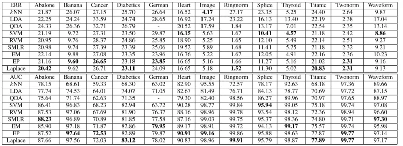
TABLE III
COMPARISON OFkNN, LDA, QDA, SVM, RVM, SMLRANDPCVMEM, EPCVMLapANDEPCVMEPON13BENCHMARKDATASETS,BY%ERROR ANDAUC. THESE RESULTS ARE THE AVERAGE OF100RUNS ON THE DATA SETS. “-”MEANS THE COVARIANCE MATRIX OF TRAINING DATA IS NOT
POSITIVE DEFINITE ANDQDACANNOT OBTAIN THE RESULTS. BOLDFACE VALUES INDICATE THE BEST PERFORMANCE IN EACH DATA SET. ERR Abalone Banana Cancer Diabetics German Heart Image Ringnorm Splice Thyroid Titanic Twonorm Waveform
kNN 21.87 26.07 27.15 25.70 26.64 16.52 4.17 27.17 23.35 5.25 24.40 2.64 9.87 LDA 22.25 24.24 33.59 24.74 28.65 16.92 17.24 23.22 16.13 13.40 22.19 2.38 17.04 QDA 24.33 26.36 32.71 26.79 - 20.52 17.59 1.84 13.17 7.01 22.54 2.35 13.14 SVM 21.19 9.72 27.31 23.50 29.87 16.15 5.63 1.67 10.41 4.57 21.18 2.42 8.86 RVM 20.95 9.76 28.37 24.86 25.85 18.90 5.25 1.65 12.10 5.49 22.14 2.51 9.27 SMLR 20.98 9.74 27.39 23.39 25.06 19.52 5.89 1.68 11.41 5.25 21.18 2.32 9.21 EM 22.14 9.88 27.08 23.35 23.96 16.76 5.22 1.67 12.05 4.91 22.16 2.36 10.23 EP 21.16 9.60 26.65 23.18 23.85 16.65 5.16 1.66 11.27 5.16 21.02 2.31 9.16 Laplace 20.42 9.62 26.71 23.11 24.09 16.65 5.18 1.52 11.30 5.02 20.83 2.31 9.13
AUC Abalone Banana Cancer Diabetics German Heart Image Ringnorm Splice Thyroid Titanic Twonorm Waveform
kNN 78.15 68.61 59.33 68.30 63.02 82.90 95.55 72.57 78.17 92.63 68.18 97.36 89.66 LDA 77.74 74.53 64.01 74.07 71.05 82.67 81.49 76.71 84.13 78.77 70.69 97.72 87.15 QDA 75.64 71.74 62.63 71.35 - 79.30 82.40 98.56 86.27 89.96 70.97 97.65 88.97 SVM 86.41 96.83 68.23 82.94 63.72 90.28 98.77 99.84 95.94 99.05 75.18 99.74 97.08 RVM 87.53 97.06 67.69 81.90 76.37 88.16 98.96 99.78 93.54 98.12 72.36 98.94 96.60 SMLR 88.23 96.89 70.89 81.85 77.58 87.16 99.03 99.75 95.37 98.36 74.80 99.71 97.30 EM 85.90 97.18 71.87 82.86 79.95 89.17 98.91 99.72 94.13 99.17 75.57 99.74 95.98 EP 87.52 97.64 72.53 82.89 79.87 90.91 99.16 99.86 95.88 98.63 77.87 99.77 97.14 Laplace 87.66 97.56 72.03 83.12 78.02 90.83 98.96 99.91 95.79 98.87 77.89 99.77 97.17
θ. For kNN, the number of nearest neighbors is selected by this methodology as well.
To select the best initialization point for PCVMEM, we train
PCVMEMwith different initializations (8initializations in this
paper) over the first five training folds of each data set. Then we choose the best initialization point6.
Table III reports the performance of these algorithms on the 13 benchmark data sets with ERR and AUC. According to this table, the performance of EPCVMLap and EPCVMEP
is similar. They outperform PCVMEM in terms of accuracy
and AUC. EPCVMLap wins 11 times over the metrics ERR
and AUC, respectively, of them seven and four wins for ERR and AUC are significant, respectively.
In comparisons with other algorithms, EPCVMLap and
EPCVMEP perform very well in terms of two different
metrics. For example, under the ERR metric it is observed that they outperforms all other methods in eight out of thirteen data sets, and comes second in three cases. They perform very well under the AUC metric, with the first place in eight cases and the second in the remaining four. Even when they fail under ERR metric on one of the data sets, e.g., Image, it can still win under the AUC metric. Although the RVM uses the Bayesian ARD framework, it seems that adopting the same prior for different classes leads to sub-optimal results.
The experimental results for SVM and SMLR are also enlightening. In most cases, the SVM and SMLR are worse than or comparable to the corresponding EPCVMLap and
EPCVMEP. The baseline algorithms, kNN and LDA/QDA,
only perform well on one data set. In all other cases, they fail to compete with the EPCVM and SVM, especially under the AUC metric.
Another interesting point is that EPCVM approaches
6With8 initializations on first five training folds, we obtain an array of parameters of dimensions8×5where the rows are the initializations and the columns are the folds. For each column, we select the results that give the smallest test error, so that the array reduces from 40 to only 5 elements. Then we select the median over those parameters.
achieve better performance by employing only a few of the data points, which has been illustrated by Table IV. In the three PCVM implementations, EPCVMEP tends to produce
small models whereas EPCVMLap often has larger models
than EPCVMEM and EPCVMEP. According to Table IV, the
number of support vectors for SVM grows almost linearly with the number of training points, while RVM consistently uses much fewer data points. EPCVMLap employs more vectors
than the RVM but much less than SVM. This observation goes in accordance with the formulation. In RVM, the weights could reach zero from both sides because of the symmetrical zero-mean Gaussian, whereas the weights in EPCVM could only converge to zero from positive side because of the truncated Gaussian prior7.
It is worth noting that the three PCVM algorithms have bet-ter performance than the RVM according to Table III. SMLR uses more vectors than three PCVM algorithms and RVM as it employed a cyclic component-wise update procedure [16], i.e., updating the weights even when they are deleted from the model, with a probability that is decreased with the number of iterations. This will be prone to include more basis functions into the model.
C. Statistical Comparisons on Single and Multiple Data Sets In order to compare EPCVMLapwith other algorithms in a
statistical context, we perform the statistical test for paired classifiers, e.g. EPCVMLap vs. SVM and EPCVMLap vs.
RVM, on each single data set. We will carry out statistical tests on these two metrics and provide the win-loss-tie summary for these metrics. The threshold of the statistical t tests is set to be 0.05.
Table V gives the win-loss-tie summary of t-test based on 13 benchmark data sets. The significance tests show that under the
7The mean of truncated Gaussian prior is √ 2
παi, which is not zero as normal Gaussian prior used in RVM.
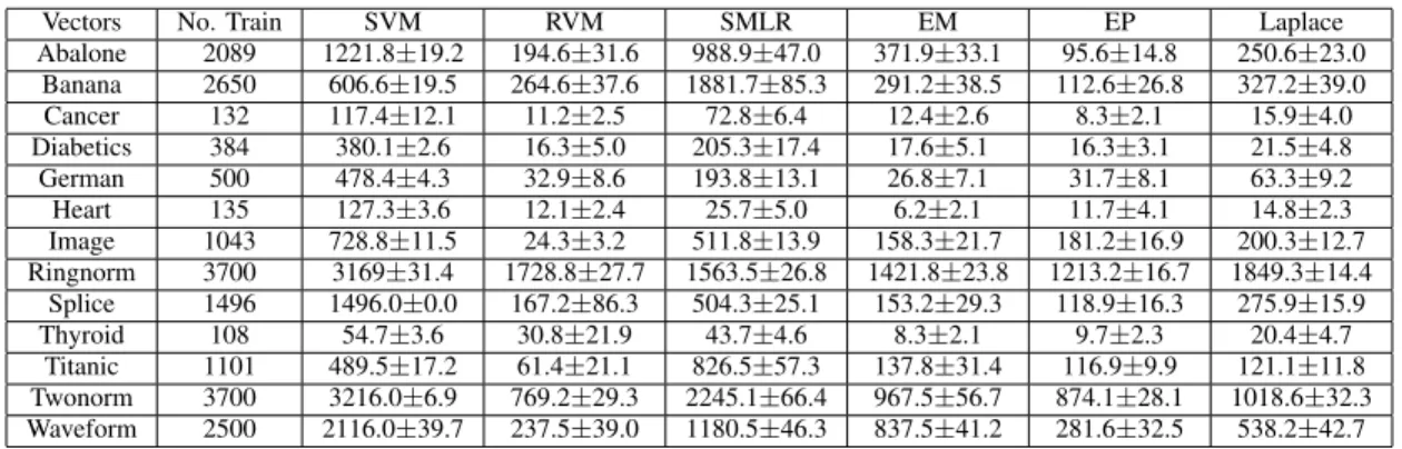
TABLE IV
COMPARISON OFSVM, RVM, SMLRANDPCVMEM, EPCVMLapANDEPCVMEPON13BENCHMARKDATASETS,BY HOW MANY VECTORS AND STANDARD DEVIATION. THESE RESULTS ARE THE AVERAGE OF100RUNS ON THE DATA SETS.
Vectors No. Train SVM RVM SMLR EM EP Laplace
Abalone 2089 1221.8±19.2 194.6±31.6 988.9±47.0 371.9±33.1 95.6±14.8 250.6±23.0 Banana 2650 606.6±19.5 264.6±37.6 1881.7±85.3 291.2±38.5 112.6±26.8 327.2±39.0 Cancer 132 117.4±12.1 11.2±2.5 72.8±6.4 12.4±2.6 8.3±2.1 15.9±4.0 Diabetics 384 380.1±2.6 16.3±5.0 205.3±17.4 17.6±5.1 16.3±3.1 21.5±4.8 German 500 478.4±4.3 32.9±8.6 193.8±13.1 26.8±7.1 31.7±8.1 63.3±9.2 Heart 135 127.3±3.6 12.1±2.4 25.7±5.0 6.2±2.1 11.7±4.1 14.8±2.3 Image 1043 728.8±11.5 24.3±3.2 511.8±13.9 158.3±21.7 181.2±16.9 200.3±12.7 Ringnorm 3700 3169±31.4 1728.8±27.7 1563.5±26.8 1421.8±23.8 1213.2±16.7 1849.3±14.4 Splice 1496 1496.0±0.0 167.2±86.3 504.3±25.1 153.2±29.3 118.9±16.3 275.9±15.9 Thyroid 108 54.7±3.6 30.8±21.9 43.7±4.6 8.3±2.1 9.7±2.3 20.4±4.7 Titanic 1101 489.5±17.2 61.4±21.1 826.5±57.3 137.8±31.4 116.9±9.9 121.1±11.8 Twonorm 3700 3216.0±6.9 769.2±29.3 2245.1±66.4 967.5±56.7 874.1±28.1 1018.6±32.3 Waveform 2500 2116.0±39.7 237.5±39.0 1180.5±46.3 837.5±41.2 281.6±32.5 538.2±42.7 TABLE V
STATISTICAL T TEST FOR13DATA SETS. FOR EACH METRIC,THE FIRST LINE IS THE WIN-LOSS-TIE SUMMARY OF THE ALGORITHM AGAINST THE
EPCVMLapBASED ON THE MEAN VALUE. THE SECOND ROW GIVES THE STATISTICAL SIGNIFICANCE WIN-LOSS-TIE SUMMARY BASED ON13
BENCHMARK DATA SETS.
Data Sets kNN LDA QDA SVM RVM SMLR EM EP
ERR Mean 2-11-0 0-13-0 0-12-0 4-9-0 0-13-0 0-13-0 2-11-0 4-7-2 Significant 1-9-3 0-11-2 0-11-1 3-4-6 0-9-4 0-5-8 0-7-6 2-2-9 AUC Mean 0-13-0 0-13-0 0-12-0 2-11-0 0-12-1 3-10-0 2-11-0 5-7-1 Significant 0-13-0 0-13-0 0-12-0 0-5-8 0-10-3 1-5-7 1-4-8 2-0-11
TABLE VI
THE MEAN RANK OF THESE ALGORITHMS UNDERERRANDAUC. Rank SVM RVM SMLR EM EP Laplace ERR 3.46 4.85 4.42 4.19 2.15 1.92 AUC 3.88 4.96 4.08 3.88 2.12 2.08
two metrics: a) PCVMEMnever significantly win EPCVMLap
under ERR and it wins once and loses four times under AUC. EPCVMEP performs similar as EPCVMLap under ERR: it
wins twice and loses twice under ERR, and it slightly outper-forms EPCVMLap under AUC by winning twice and never
loses. b) The differences between RVM and the EPCVMLap
are greater: RVM never wins under ERR and AUC. c) SVM wins three time and lose four times under ERR, and never wins under AUC. d) The experimental results also reveal that these baseline algorithms under-perform significantly against other algorithms.
In order to compare multiple algorithms based on multiple data sets, it is a common approach to count the number of times an algorithm performs better, worse or equal to the others. However, this method might not be reliable since it puts an arbitrary threshold of 0.05 or 0.10 on what counts and what does not for each data set [7]. Statistical tests on multiple data sets for multiple algorithms are preferred for comparing different algorithms over multiple data sets. In order to conduct statistical tests over multiple data sets, we perform the Friedman test [12] with the corresponding post-hoc tests. The Friedman test is a non-parametric equivalent of the repeated-measures analysis of variance (ANOVA) under the null hypothesis that all the algorithms are equivalent and so their ranks should be equal. This paper uses an improved Friedman test proposed by Iman and Davenport [13].
TABLE VII
FRIEDMAN TESTS WITH THE CORRESPONDING POST-HOC TESTS, BONFERRONI-DUNN,TO COMPARE CLASSIFIERS FOR MULTIPLE DATA
SETS. THE THRESHOLD IS0.10,ANDq0.10= 2.326.
Metrics Friedman test CD0.10 SVM RVM SMLR EM EP
ERR 0.00 1.71 1.54 2.92 2.50 2.27 0.23 AUC 0.00 1.71 1.81 2.88 2.00 1.81 0.04
The Friedman test is carried out to test whether all the algorithms are equivalent. If the test result rejects the null hypothesis, i.e. these algorithms are equivalent, we can pro-ceed to a post-hoc test. The power of the post-hoc test is much greater when all classifiers are compared with a control classifier and not among themselves. We do not need to make pairwise comparisons when we in fact only test whether a newly proposed method is better than the existing ones.
Based on this point, we would like to choose the EPCVMLap as the control classifier to be compared with.
Since the baseline classification algorithms are not compa-rable to SVM, RVM, SMLR, PCVMEM, EPCVMEP and
EPCVMLap, this section will analyze only six algorithms:
SVM, RVM and SMLR, PCVMEM and EPCVMEP against
the control classifier EPCVMLap.
The Bonferroni-Dunn test [7] is used as post-hoc tests when all classifiers are compared to the control classifier. The performance of pairwise classifiers is significantly different if the corresponding average ranks8 differ by at least the critical difference (CD)
CD=qα
√
j(j+ 1)
6T , (11)
wherej is the number of algorithms,T is the number of data sets and critical valuesqα can be found in [7]. For example,
when j = 6, q0.10 = 2.326, where the subscript 0.10 is the
threshold value.
Table VI lists the mean rank of these algorithms under the two metrics: ERR and AUC. Table VII gives the Friedman test results. Since we employ the same threshold0.10for all three
8We rank these algorithms based on the metric on each data set and record the ranking of each algorithm as 1, 2 and so on. Average ranks are assigned in case of ties. The average rank of one algorithm is obtained by averaging over all of data sets. Please refer to Table VI for the mean rank of these algorithms under different metrics.
metrics, the critical difference CD = 1.71, wherej = 6and T = 13, is the same for these metrics. Several observations can be made from our results.
First, under the ERR metric, the differences between EPCVMLap and RVM, SMLR, PCVMEM, are greater than
the critical difference, so the differences are significant, which means the EPCVMLap is significantly better than RVM,
SMLR and PCVMEM in this case. We could not detect any
significant differences between SVM and EPCVMEP. The
correct statistical statement would be that the experimental data are not sufficient to reach any conclusion regarding the difference between EPCVMLap and SVM/EPCVMEP.
Second, EPCVMLap significantly outperforms all other
al-gorithms under the AUC metric except EPCVMEP. Since the
AUC metric requires relative accurate scores to discriminate positive and negative instances [10], EPCVMLapsucceeds by
generating the probabilistic outputs. Another reason is that AUC is insensitive to the class skew/distribution [10] and some data sets used in this paper are imbalanced. In this way, EPCVMLap and EPCVMEP perform well on these
unbal-anced data sets by considering different priors for different classes and thus have better scores under the AUC metric. SMLR generates point estimation based MAP, therefore it does not perform very well on AUC metric.
There are two major reasons why the two implementations of EPCVM, i.e. EPCVMLap and EPCVMEP, perform better
than others.
1) The robustness and sparseness are generated by the trun-cated Gaussian priors. These priors control the model complexity by including appropriate sparseness, and thus improve the model generalization.
2) As AUC prefers probabilistic outputs than hard decisions and it is insensitive to class unbalance, EPCVMLapand
EPCVMEP provide probabilistic outputs to assess the
uncertainty for the predictions and perform well on these unbalanced data sets, which explain why EPCVMLap
and EPCVMEP are good under the AUC metric.
Al-though the RVM also provides probabilistic outputs, it adopts Gaussian prior for training points belonging to both classes over weights and thus leads to inferior results.
D. Computational Complexity
The computational complexity and memory storage for PCVMEM isO(N3)andO(N2), respective, where N is the
number of training points. The PCVMEM model will initially
includeall, i.e.N, basis functions in the beginning and reduce the model size gradually. This will leads to longer training times and larger memory usage. In addition, to address the common problems of EM, including sensitivity to initializa-tions and convergence to local minima, the usual approach is to run the algorithm multiple times from different initialization points and choose the best one based on validation data, which will even increase the computational requirement in practice. In EPCVMLap, the update rules of w andbinvolve
inver-sion of a matrix. The Cholesky decomposition is used in the practical implementation of the inversion to avoid numerical
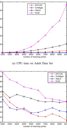
10000 2000 3000 4000 5000 6000 7000 8000 9000 10000 2000 4000 6000 8000 10000 12000
number of trainning points
CPU Time (s)
EPCVM SVMlight SMLR RVM
(a) CPU time on Adult Data Set
1000 2000 3000 4000 5000 6000 7000 8000 9000 10000 0.15 0.152 0.154 0.156 0.158 0.16 0.162 0.164 0.166 0.168 0.17
number of trainning points
Err rate (%)
EPCVM SVMlight SMLR RVM
(b) Error Rate on Adult Data Set
Fig. 4. Comparison of CPU time and the error rate of EPCVMLap, SVM,
SMLR and RVM on Adult data set.
instability, which has the computational complexity O(M3)
and memory storage O(M2), where M is the number of
non-zero basis functions and M << N. In EPCVMLap,
we will start when M = 1, and include basis functions step by step, i.e. increase M. As reported in Table IV, the final EPCVMLap model usually has a small number of basis
functions, i.e. a small M. This procedure will dramatically reduce the computational complexity.
Classical SVM algorithms has a time complexity ofO(N3),
whereN is the number of training points, but the computa-tional complexity of SVM can be reduced to approximately O(N2.1) for sequential minimal optimization (SMO) like al-gorithms [23], which breaks the large quadratic programming (QP) problem into a series of smallest possible QP problems. The training algorithm of SVMlight has been optimized in many aspects [15], and it is even faster than the popular SMO algorithm for training SVM. The time complexity of each iteration in SVMlight is O(N DL), where D is the number of input features (input dimensionality) and L is a (regularization) parameter to control the number of rows of the Hessian to be computed in each iteration. The empirical time complexity of SVMlightisO(N1.7∼2.0)[15], hence it is faster than EPCVMLap. Since EPCVMLap is implemented in
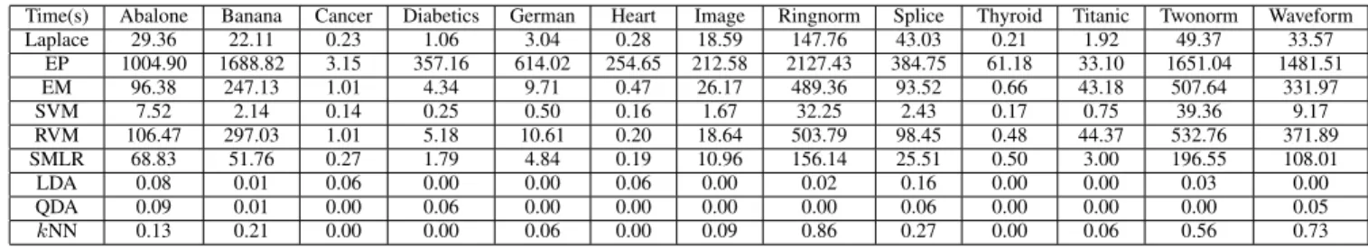
TABLE VIII
CPU TIME OF THEEPCVMLapANDEPCVMEP, PCVMEM, SMLR, SVM, RVM, LDA, QDA,kNNON13 DATASETS IN SECONDS. RESULTS ARE AVERAGED OVER100RUNS.
Time(s) Abalone Banana Cancer Diabetics German Heart Image Ringnorm Splice Thyroid Titanic Twonorm Waveform Laplace 29.36 22.11 0.23 1.06 3.04 0.28 18.59 147.76 43.03 0.21 1.92 49.37 33.57 EP 1004.90 1688.82 3.15 357.16 614.02 254.65 212.58 2127.43 384.75 61.18 33.10 1651.04 1481.51 EM 96.38 247.13 1.01 4.34 9.71 0.47 26.17 489.36 93.52 0.66 43.18 507.64 331.97 SVM 7.52 2.14 0.14 0.25 0.50 0.16 1.67 32.25 2.43 0.17 0.75 39.36 9.17 RVM 106.47 297.03 1.01 5.18 10.61 0.20 18.64 503.79 98.45 0.48 44.37 532.76 371.89 SMLR 68.83 51.76 0.27 1.79 4.84 0.19 10.96 156.14 25.51 0.50 3.00 196.55 108.01 LDA 0.08 0.01 0.06 0.00 0.00 0.06 0.00 0.02 0.16 0.00 0.00 0.03 0.00 QDA 0.09 0.01 0.00 0.06 0.00 0.00 0.00 0.00 0.06 0.00 0.00 0.00 0.05 kNN 0.13 0.21 0.00 0.00 0.06 0.00 0.09 0.86 0.27 0.00 0.06 0.56 0.73 sets.
The computational complexity of EPCVMEP isO(N M3),
which is the highest in the three implementations of PCVM. The long time consumed by EPCVMEP has been confirmed
by Table VIII. In this paper, the aim to develop EPCVMEP is
to confirm the effectiveness of EPCVMLap, and to compare
the approximation accuracy of Laplace approximation. Since the computational complexity of EPCVMEP is higher, it
is applicable for relatively small problems in the practical situations with the benefits to obtain compact models with fewer basis functions and the estimation of leave-one-out error in the training.
Table VIII shows the average CPU time of EPCVMLap,
EPCVMEP, PCVMEM, SMLR, SVM, RVM, LDA, QDA,
kNN on 13 data sets in seconds. Results are averaged over 100 runs. Note that in Table VIII, we do not record the cross validation time for parameter optimization in these algorithms. To further study the computational effectiveness of EPCVMLap9, SVM, SMLR and RVM, a relatively large data
set, Adult from UCI machine learning repository, has been employed.
In Figure 4, the CPU time and the error rate of these algorithms on Adult data have been reported. As SVMlight [15] has been used to implement SVM, in which sequential minimal optimization algorithm (SMO) and the optimization for large problems have been implemented. This is the rea-son why SVMlight is the fastest algorithm. EPCVMLap is
programmed in Matlab and there is still room to improve its computational complexity by using C.
RVM and SMLR do not scale well with increased data points. SMLR employed a cyclic component-wise update procedure [16] and it will consider the weights even when they are deleted from the model. Therefore, the computation time becomes higher.
Figure 4 confirmed the computational effectiveness and the performance of EPCVMLap, as it scales well with the number
of training points without compromising the performance. The computational environment is Windows 7 with Intel Xeon QuadCore 3.10GHz CPU and 8GB RAM. The source codes of RVM and SMLR are obtained from Tipping’s web-site10, and Princeton’s multi-voxel pattern analysis toolbox11,
9The computational complexity of EPCVM
EP is much higher than
EPCVMLap, SVM, SMLR and RVM. Therefore, we do not report the
performance of EPCVMEP on the Adult data set.
10http://www.miketipping.com/
11http://code.google.com/p/princeton-mvpa-toolbox/
respectively. EPCVMLapand EPCVMEP are implemented in
MATLAB.
V. SPARSITY ANDGENERALIZATION
In this section we use Rademacher complexity [20] to investigate the relationship between the generalization bound for EPCVM and model sparsity.
Rademacher complexity quantifies “complexity” of function classes. LetF be a class of real-valued functions defined on X. The empirical Rademacher complexity of a functional class F on a data setD={(x1, y1),· · ·,(xN, yN)} is defined as
ˆ RN(F, D) = 2 NEς [ sup f∈F N ∑ i=1 ςif(xi) ]
whereς = (ς1, ς2,· · · , ςN) is a vector random variable with
elements independent binary random Rademacher variables such thatP(ςi= +1) =P(ςi=−1) = 1/2 for allςi.
Assume that there is a distributionP(x, y)that generates the data items (i.e.P(x, y)represents the environment producing the data). The data set D = {(x1, y1),· · · ,(xN, yN)} is
generated i.i.d. form from P(x, y), i.e. D is generated from the product distribution G(D), G = PN. The Rademacher
complexity ofF is then RN(F) =EG(D) [ ˆ RN(F, D) ] . (12) Rademacher complexity can be used to formulate general-ization bound, as illustrated by the following theorem.
Theorem 1: [16], [20] Given a dataset D =
{(x1, y1),· · · ,(xN, yN)}, for posterior distribution q(w)
over the parameters w(see section II-D), let f(x, q) =Eq(w)[sign(wTϕ(x))].
Fors >0, letR(emps) be the empirical loss defined as
R(emps) [f, D] = 1 N N ∑ n=1 ls(ynf(xn, q)),
where the loss function12l
s(a) =min(1, max(0,1−a/s))is
(1/s)-Lipschitz. Consider arbitrary scalarsρ >0,r >0. Then, for ϑ∈ (0,1), with probability at least1−ϑ over draws of
12For wrong classifications (a < 0), the loss is equal to 1. For correct classifications, s plays the role of the classification margin - even if the classification is correct (a >0), ifais bellows, a linearly scaled penalty 1−a/sis still applied. The loss is zero only fora≥s.
training sets from G, the following bound for generalization error holds: P(yf(x, q) < 0)≤R(emps) [f, D] +2 s √ 2 ˜ρ(q) N + √ ln logrrρ˜ρ(q)+12ln1ϑ N , (13) and ˜ ρ(q) =r·max(KL(q||p), ρ), (14) whereKL(q||p)13 is the Kullback-Leibler divergence from the posterior qto the prior pover parametersw.
Note that the prior is integral part of our model, its hyperparameter α is modified during training. The Bayesian predictions of our model are based on the posterior over the weights that is in turn obtained from the optimized prior α. In this section we will denote the initial and optimized hyperparameter by α0 and α, respectively. Based on the
theorem, the generalization bound of EPCVM is related to the empirical loss and KL(q||p). Given the same empirical loss, the generalization bound is tight provided KL(q||p) is small. In the following, we will investigate the termKL(q||p).
A. Kullback-Leibler Divergence from Posterior to Prior
0 1 2 3 4 5 0 5 10 0 5 10 15 20 25 30 ˆ αi w i KL Divergence
Fig. 5. An illustration of KL divergence between truncated posterior and truncated Gaussian prior.
The Kullback–Leibler (KL) divergence is a non-symmetric measure of the difference between two probability distri-butions. In this paper, posterior over weights is obtained through Laplace approximation q˜(w). This posterior, q˜(w), is a multivariate Gaussian with unbounded support. However, the prior is truncated to positive quadrant. The probability mass of q˜ in the positive quadrant is A0 =
∫∞
0 q˜(w)dw.
Provided A0 is sufficiently high, we can approximate q˜ by
its renormalized version with support in the positive quadrant, q(w) = ˜q(w)/A0.
13known as Bayesian surprise [14]
The KL divergence from q(w) to prior p(w|α0) can be calculated as KL(q(w)∥p(w|α0)) = ∫ ∞ 0 ˜ q(w) A0 lnq˜(w) A0 dw − ∫ ∞ 0 ˜ q(w) A0 lnp(w|α0)dw = 1 A0 ∫ ∞ 0 ˜ q(w) ln q˜(w) p(w|α0)dw −lnA0.
In this paper, we follow [16] and adopt the independence assumption on the posterior. Then (see Appendix A.5 of [5]), DKL = KL(q(w)∥p(w|α0)) (15) = ∑ i,wi̸=0 1 2 [ α0,i αi −1 + ln ( αi α0,i ) +α0,iw2i ] +(2παi)−1/2(α0,i+αi)wi erf cx ( −wi √ αi/2 ) −ln(erf c(−wiαi 2 )) ,
whereerf cx(a) =ea2erf c(a).
Since A0,i= ∫ ∞ 0 ˜ q(wi)dwi= 1 2erfc ( −wi √ αi 2 ) ,
DKL can be rewritten as follows:
DKL= ∑ i,wi̸=0 1 2 [ α0,i αi −1 + ln ( αi α0,i ) +α0,iw2i ] +(2παi)−1/2(α0,i+αi)wi 2 exp(αiw2i/2) A−0,i1−ln (A0,i) + ln ( erf c ( −wi √ αi/2 ) 2·erf c(−wiαi/2) ) .
To show the characteristics of the KL divergence, in Figure 5 we illustrate the contributions of individual terms by fixing the initial hyperparameter priors to α0,i = 0.5 (the value
used in our experiments). Two observations can be made: First, DKL is much more sensitive to weight values wi
than to the optimized hyperparameters αi. Second, DKL is
minimized for vanishing weights wi. As discussed above,
for comparable empirical errors, smaller DKL is desirable.
Therefore, employing truncated Gaussian priors in EPCVM to encourage sparsity by regularizing the weights to be smaller may have beneficial effects on the generalization, provided enough positive weights are preserved to ensure sufficient flexibility of the model.
Based on equations (13) and (15), the generalization bound of the EPCVM is a function of both the empirical loss term and the sparsity, represented by minimizing DKL. According to
Equation (14), trying to pushDKLto very small values beyond
ρis not desirable. Therefore, adequate sparsity is preferred in EPCVM, which matches our intuition regarding the nature of the generalization bound: If EPCVM chooses a non-sparse solution, the bounds might be loose; in contrast, if EPCVM chooses a proper sparse solution that can balance the empirical loss and the KL divergenceDKL, the bounds might be tight.